The quantum-classical transition in thermally seeded parametric downconversion

Abstract

We address the pair of conjugated field modes obtained from parametric-downconversion as a convenient system to analyze the quantum-classical transition in the continuous variable regime. We explicitly evaluate intensity correlations, negativity and entanglement for the system in a thermal state and show that a hierarchy of nonclassicality thresholds naturally emerges in terms of thermal and downconversion photon number. We show that the transition from quantum to classical regime may be tuned by controlling the intensities of the seeds and detected by intensity measurements. Besides, we show that the thresholds are not affected by losses, which only modify the amount of nonclassicality. The multimode case is also analyzed in some detail.

1 Introduction

The boundary between quantum and classical physics has been controversial [1, 2, 3, 4, 5, 6, 7, 8, 9] ever since the early days of quantum mechanics. Nevertheless, the solution to this problem is very important for several fundamental issues in quantum and atomic optics and, more generally, in quantum measurement theory [10, 11]. More recently, with the development of quantum technology, the issue gained new interest since nonclassical features, in particular entanglement, represent practical resources to improve quantum information processing.

As a matter of fact, quantum decoherence, i.e. the dynamical suppression of quantum interference effects, cannot be the unique criterion to define a classical limit [12], which should emerge from an operational approach suitably linked to measurement schemes [13, 14, 15, 16, 17, 18, 19, 20, 21, 22, 23, 24, 25, 26, 27, 28, 29]. To this aim here we address the bipartite system made by the pair of field modes obtained from parametric downconversion (PDC) as a convenient physical system to analyze the quantum-classical transition in the continuous variable regime. We consider a PDC process seeded by thermal radiation, a scheme that we already investigated in ghost-imaging/diffraction experiments [30, 31, 32] and where it has been shown that both entanglement and intensity correlations may be tuned upon changing the intensities of the seeds [31]. This, in turn, puts forward the PDC output as a natural candidate to investigate the quantum-classical transitions in an experimentally feasible configuration. We focus on some relevant parameters employed to point out the appearance of quantum features, namely sub-shot-noise correlations, negativity and entanglement. We analyze at varying the mean photon numbers of the interacting fields the different nonclassicality thresholds that appear. Remarkably, the corresponding transitions from classical to quantum domain may be observed experimentally by means of intensity measurements, thus avoiding full state reconstruction by homodyne or other phase-sensitive techniques [33, 34].

The paper is structured as follows. In the next section we review the PDC process, establish notation and introduce the nonclassicality parameters we are going to analyze. In Section 3 we analyze the effect of losses, whereas in Section 4 we discuss the generalization of our analysis to the multimode case. Finally, Section 5 closes the paper with some concluding remarks.

2 Parametric downconversion with thermal seeds

The evolution of a pair of field modes under PDC is described by the unitary operator ${U}_{\kappa}=\exp(i\kappa{a_{1}}{a_{2}}+h.c.)$, where $\kappa$ is the coupling constant and $a_{j}$ are the mode operators $(j=1,2)$. In the following we consider the two modes initially in a thermal state, i.e. excited in a factorized thermal state $\boldsymbol{\nu}=\nu_{1}\otimes\nu_{2}$, $\nu_{j}=\sum_{n=0}^{\infty}p_{j}(n)~{}|n\rangle_{jj}\!\langle n|$ being a single-mode thermal state with $\mu_{j}$ mean number of photons, i.e. $p_{j}(n)=\mu_{j}^{n}(1+\mu_{j})^{-(n+1)}$. The density matrix at the output is given by ${{\boldsymbol{\varrho}}_{\kappa}}={U}_{\kappa}\>\boldsymbol{\nu}\>{U}^{\dagger}_{\kappa}$, whereas the output modes are given by $A_{j}={U}_{\kappa}^{{\dagger}}{a}_{j}{U}_{\kappa}=\alpha a_{j}+e^{i\varphi}\beta a_{j^{\prime}}^{\dagger}$ (with $j=1,2$ and $j\neq j^{\prime}$) where $\alpha=\cosh|\kappa|$, $\beta=\sinh|\kappa|$ and $\varphi$ is the coupling (i.e. pump) phase. The statistics of the two output modes, taken separately, are those of a thermal state [31], i.e. $\langle{n}_{j}\rangle=\mu_{j}+\mu_{\kappa}(1+\mu_{1}+\mu_{2})$, $\langle\Delta n_{j}^{2}\rangle=\langle{n}_{j}\rangle(\langle{n}_{j}\rangle+1)$, where $n_{j}=a_{j}^{{\dagger}}a_{j}$ and $\mu_{\mathrm{\kappa}}=\sinh^{2}|\kappa|$ is the mean number of photons due to spontaneous PDC; the symbols $\langle...\rangle$ and $\Delta$ denote $\langle{O}\rangle=\mathrm{Tr}[{O}{\varrho}]$ and $\Delta{O}={O}-\langle{O}\rangle$, respectively. Notice that the case of vacuum inputs, $\boldsymbol{\nu}=|0\rangle\langle 0|_{1}\otimes|0\rangle\langle 0|_{2}$, corresponds to spontaneous downconversion, i.e. to the generation of the so-called pure twin-beam state (TWB) $|{\boldsymbol{\psi}}_{\kappa}\rangle\rangle=U_{\kappa}|0\rangle=\alpha^{-1}\sum_{n}(\beta/\alpha)^{n}\>|n\rangle\otimes|n\rangle$ [35].

2.1 Intensity correlations

The shot-noise limit (SNL) in a photodetection process is defined as the lowest level of noise that can be achieved by using semiclassical states of light [36, 37, 38], that is Glauber coherent states. On the other hand, when a noise level below the SNL is observed, we have a genuine nonclassical effect. For a two-mode system if one measures the photon number of the two beams and evaluates the difference photocurrent $H=n_{1}-n_{2}$ the SNL is the lower bound to the fluctuations $\langle\Delta H^{2}\rangle$ that is achievable with classically coherent beams, i.e. $\langle\Delta H^{2}\rangle=\langle{n}_{1}\rangle+\langle{n}_{2}\rangle$.

Let us consider a simple measurement scheme where the modes at the output of the PDC crystal are individually measured by direct detection and the resulting photocurrents are subtracted from each other to build the difference photocurrent. We have quantum noise reduction, i.e. violation of the SNL, when $\langle\Delta H^{2}\rangle<\langle{n}_{1}\rangle+\langle{n}_{2}\rangle$, that is [31]

$$\mu_{1}^{2}+\mu_{2}^{2}<2\mu_{\kappa}(1+\mu_{1}+\mu_{2})$$ (1)

In order to quantify intensity correlations and to evaluate the amount of violation of the SNL we introduce the parameter

$$\gamma_{c}=1-\frac{\langle\Delta H^{2}\rangle}{\langle{n}_{1}\rangle+\langle{n}_{2}\rangle}.$$ (2)

The value $\gamma_{c}=0$ corresponds to noise at the SNL, whereas the presence of nonclassical intensity correlations leads to $0<\gamma_{c}\leq 1$. For the pair of modes at the output of the PDC crystal we obtain

$$\gamma_{c}=\frac{2~{}\mu_{\kappa}(1+\mu_{1}+\mu_{2})-\mu_{1}^{2}-\mu_{2}^{2}}{2~{}\mu_{\kappa}(1+\mu_{1}+\mu_{2})+\mu_{1}+\mu_{2}}.$$ (3)

The maximal violation of SNL is achieved by the TWB state ($\mu_{1}=\mu_{2}=0$), while upon increasing the intensity of at least one of the seeding fields the SNL is eventually reached.

2.2 Negativity

The nonclassical behaviour of a set of light modes has been often related to the negativity of the Glauber-Sudarshan P-function, which, in turn, prevents the description of the systems as a classical statistical ensemble. Here, in order to quantify negativity in terms of the photon number distribution, we employ the criterion introduced by Lee [39, 40], which represents the two-mode generalization of the Mandel’s criterion of nonclassicality [41] for single-mode beams and, in turn, implies the negativity of the P-function. According to Lee [39, 40], a bipartite system shows nonclassical behaviour if the inequality

$$\langle n_{1}(n_{1}-1)\rangle+\langle n_{2}(n_{2}-1)\rangle-2\langle n_{1}n_{2}\rangle<0$$ (4)

is satisfied. For the PDC output state, the condition in Eq. (4) corresponds to $\mu_{1}^{2}+\mu_{2}^{2}-\mu_{1}\mu_{2}<\mu_{\kappa}(1+\mu_{1}+\mu_{2})$. As we did in the case of intensity correlations, we define a parameter quantifying the amount of negativity

$$\gamma_{n}=1-\frac{\langle\Delta H^{2}\rangle+(\langle{n}_{1}\rangle-\langle{n}_{2}\rangle)^{2}}{\langle{n}_{1}\rangle+\langle{n}_{2}\rangle}.$$ (5)

We have $0<\gamma_{n}\leq 1$, with $\gamma_{n}=1$ corresponding to maximum nonclassicality. For the PDC output state we obtain

$$\gamma_{n}=2~{}\frac{\mu_{\kappa}(1+\mu_{1}+\mu_{2})-\mu_{1}^{2}-\mu_{2}^{2}+\mu_{1}\mu_{2}}{2~{}\mu_{\kappa}(1+\mu_{1}+\mu_{2})+\mu_{1}+\mu_{2}}.$$ (6)

Again the most nonclassical state is the TWB state ($\mu_{1}=\mu_{2}=0$), whereas by increasing the intensity of at least one of the seeding field, the positive P-function region is eventually reached.

2.3 Entanglement

The PDC process provides pairwise entanglement in the two modes. In the spontaneous process the output state is entangled for any value of $\mu_{\kappa}\neq 0$, whereas for thermally seeded PDC the degree of entanglement crucially depends on the intensity of the seeding fields [31]. For a bipartite Gaussian state, entanglement is equivalent to the positivity under partial transposition (PPT) condition [42], which may be written in terms of the smallest partially transposed symplectic eigenvalue. Thus, seeded PDC produces an entangled output state if and only if [31]

$$\mu_{1}\mu_{2}-\mu_{\kappa}(1+\mu_{1}+\mu_{2})\geq 0.$$ (7)

Remarkably, entanglement properties of the state ${\boldsymbol{\varrho}}_{\kappa}$ can be verified by intensity measurements independently performed on the two modes. In fact, with an ideal detection system, the inequality

$$\langle\Delta H^{2}\rangle-(\langle{n}_{1}\rangle-\langle{n}_{2}\rangle)^{2}\leq\langle{n}_{1}\rangle+\langle{n}_{2}\rangle.$$ (8)

reproduces exactly the entanglement condition in Eq. (7). Therefore, the amount of the violation of the separability boundary may be quantified by means of the parameter

$$\gamma_{e}=1-\frac{\langle\Delta H^{2}\rangle-(\langle{n}_{1}\rangle-\langle{n}_{2}\rangle)^{2}}{\langle{n}_{1}\rangle+\langle{n}_{2}\rangle}.$$ (9)

$\gamma_{e}=0$ corresponds to the boundary between separable and entangled states. For the PDC output ${\boldsymbol{\varrho}}_{\kappa}$ we obtain

$$\gamma_{e}=2~{}\frac{\mu_{\kappa}(1+\mu_{1}+\mu_{2})-\mu_{1}\mu_{2}}{2~{}\mu_{\kappa}(1+\mu_{1}+\mu_{2})+\mu_{1}+\mu_{2}}.$$ (10)

Maximally entangled states ($\gamma_{e}=1$) thus correspond to the TWB ($\mu_{1}=\mu_{2}=0$), whereas entanglement is degraded in the presence of thermal seeds. Notice, however, that if one of the two modes at the input is the vacuum, the state is always entangled irrespective of the intensity of the other seeds.

In Fig. 1 we show the nonclassicality regions in terms of the seeding, $\mu_{j}$, $j=1,2$, and downconversion, $\mu_{k}$, mean photon numbers, i.e. the triples $(\mu_{1},\mu_{2},\mu_{\kappa})$ for which the parameters $\gamma$ lie in the interval $0<\gamma\leq 1$. As it is apparent from the plot, a hierarchy of nonclassicality concepts and thresholds naturally appears. The most stringent criterion of nonclassicality corresponds to negativity, followed by sub-shot-noise intensity correlations and then by entanglement.

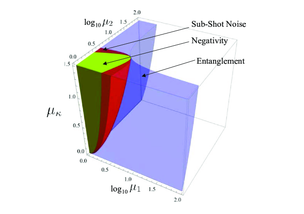
Figure 1: (Color online) Nonclassicality regions, i.e. regions for which $0<\gamma<1$, in terms of $\mu_{1}$, $\mu_{2}$, and $\mu_{\kappa}$ for the three $\gamma$ parameters introduced in the text. As it is apparent from the plot, a hierarchy of regions and bounds appears. The wider region (red$+$green$+$blue) identifies the values of the $\mu$’s leading to an entangled output ($0<\gamma_{e}<1$) from the PDC. The intermediate (red$+$green) corresponds to nonclassical intensity correlations ($0<\gamma_{c}<1$), whereas the narrower internal region (green) is for negativity ($0<\gamma_{n}<1$).

We can express the thresholds for the appearance of nonclassicality as conditions on the mean number of photons resulting from the downconversion process

$${\gamma_{n}=0} \rightarrow \mu_{\kappa}^{n}=\frac{\mu_{1}^{2}+\mu_{2}^{2}-\mu_{1}\mu_{2}}{1+\mu_{1}+\mu_{2}}\quad$$ (11)

$${\gamma_{c}=0} \rightarrow \mu_{\kappa}^{c}=\frac{\mu_{1}^{2}+\mu_{2}^{2}}{2(1+\mu_{1}+\mu_{2})}$$ (12)

$${\gamma_{e}=0} \rightarrow \mu_{\kappa}^{e}=\frac{\mu_{1}\mu_{2}}{1+\mu_{1}+\mu_{2}}\quad$$ (13)

In other words, being negative-nonclassical is a sufficient condition to have sub-shot-noise intensity correlation. Moreover, either of the two (negativity and sub-shot-noise) is a sufficient condition for entanglement, i.e. $\mu_{\kappa}^{c}>\mu_{\kappa}^{n}>\mu_{\kappa}^{e}$ for any value of $\mu_{1}$ and $\mu_{2}$. Remarkably, the three nonclassicality conditions collapse into a single one when the seeding intensities are equal $\mu_{1}=\mu_{2}$ and differ by terms up to the second order in $|\mu_{1}-\mu_{2}|$ in the neighbourhood of this condition. It is already evident in Fig. 1, as well as in Fig. 2, where we show the three parameters as function of the seeding intensities for different values of $\mu_{\kappa}$, that the stronger is the spontaneous PDC (large $\mu_{\kappa}$) the larger is the number of thermal photons that can be injected while preserving negativity and hence sub-shot-noise correlations and entanglement.

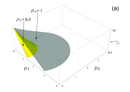
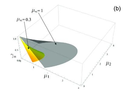
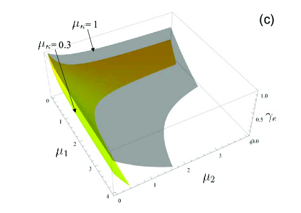
Figure 2: (Color online) Nonclassicality parameters $\gamma_{c}$, $\gamma_{n}$ and $\gamma_{e}$ evaluated for $\mu_{\kappa}=0.3$ (yellow) and $\mu_{\kappa}=1$ (black) as a function of $\mu_{1}$ and $\mu_{2}$.

3 Effect of losses

In order to see whether the nonclassicality thresholds identified in the previous section may be investigated experimentally, one should take into account losses occurring during propagation, which generally degrade quantum features, and non-unit quantum efficiency in the detection stage, which may prevent the demonstration of nonclassicality. The two mechanisms may be subsumed by an overall loss factor $\tau$ [43, 44] using a beam splitter model [45, 46] in which the signal enters one port and the second one is left unexcited. Upon tracing out the second mode we describe the loss of photons during the propagation and the detection stage. In the following we assume equal transmission factor for the two channels and evaluate the nonclassicality parameters in the presence of losses.

Upon assuming that dark counts have been already subtracted, the positive operator-valued measure (POVM) of each detector is given by a Bernoullian convolution of the ideal number operator spectral measure. The moments of the distribution are evaluated by means of the operators

$$N_{j}(\tau,p)=\sum_{n=0}^{\infty}(1-\tau)^{n}\>G_{j}(p,n)\>|n\rangle\langle n|$$ (14)

where $G_{j}(p,n)=\sum_{m=0}^{n}{n\choose m}\left(\frac{\tau}{1-\tau}\right)^{m}\!\!m^{p}$. Of course, since $N_{j}(\tau,p)$ are operatorial moments of a POVM, in general we have $N_{j}(\tau,p)\neq N_{j}(\tau,1)^{p}$, with the first two moments given by

$$N_{j}(\tau,1)=\tau n_{j}$$ (15)

$$N_{j}(\tau,2)=\tau^{2}n_{j}^{2}+\tau(1-\tau)n_{j}\>.$$ (16)

Upon inserting the above expressions in the nonclassicality parameters (i.e. replacing $n_{j}$ and $n_{j}^{2}$ by $N_{j}(\tau,1)$ and $N_{j}(\tau,2)$ respectively), we obtain that, for all of them, the inclusion of losses results in a simple re-scaling

$$\gamma_{i}(\tau)=\tau\,\gamma_{i}(\tau=1)\qquad i=c,n,e\>.$$ (17)

In other words, the effect of losses is that of decreasing the amount of nonclassicality, whereas the thresholds for the quantum-classical transitions are left unaffected. This also means that the twin-beam still corresponds to the maximal violation of classicality condition independently of the kind of nonclassicality parameter we are taking into account. These are shown in Fig. 3, where the parameters $\gamma$ for $\tau=0.5$ are compared with those in ideal condition for a fixed value of the PDC gain.

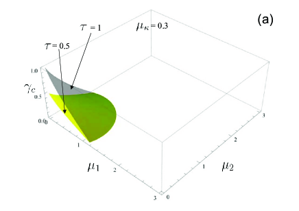
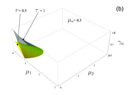
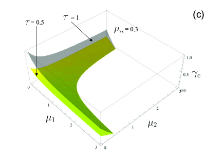
Figure 3: (Color online) Nonclassicality parameters $\gamma_{c}$, $\gamma_{n}$ and $\gamma_{e}$ evaluated for $\tau=0.5$ (yellow) and in the absence of losses ($\tau=1$, black) as a function of $\mu_{1}$ and $\mu_{2}$, with $\mu_{\kappa}=0.3$.

4 The multimode case

The (quantum) correlations introduced by the PDC process are intrinsically pairwise and thus no qualitative differences should be expected when considering the multimode case. On the other hand, the expression of the parameters $\gamma$ does depend on the number of modes and thus it is worth explicitly addressing the multimode case [31]. Besides, from the experimental point of view, this is a situation often encountered in travelling-wave PDC pumped by pulsed lasers.

The evolution operator for the multimode case can be rewritten in terms of the operators ${S}_{\xi}=(\kappa_{\xi}{a}_{1,\xi}{a}_{2,\xi}+h.c.)$ as ${U}_{M}=\bigotimes_{\xi=1}^{M}\>e^{i{S}_{\xi}}$ thus emphasizing the pairwise structure. In our analysis we focus on the case in which all the modes are seeded with uncorrelated multi-mode thermal fields with $\mu_{j,\xi}$ mean photon number per mode

$${\boldsymbol{\nu}_{M}}=\bigotimes_{\xi=1}^{M}\left({\nu}_{1,\xi}\otimes{\nu}_{2,\xi}\right)\qquad{\nu}_{j,\xi}=\sum_{n=0}^{\infty}p_{j,\xi}(n)~{}|n\rangle_{j,\xi}{}_{\xi,j}\langle n|\>,$$

where $j=1,2$. The density matrix at the output is thus given by

$${\boldsymbol{\varrho}}_{M}=U_{M}\boldsymbol{\nu}_{M}U^{\dagger}_{M}=\bigotimes_{\xi}\left[e^{i{S}_{\xi}}\>\left(\nu_{1,\xi}\otimes\nu_{2,\xi}\right)\>e^{-i{S}_{\xi}}\right]\>,$$ (18)

and the calculation for each pair of coupled modes is completely analogous to that performed in the first Section (see also [31]). The Heisenberg evolution of modes is

$${A}_{j,\xi}={U}^{{\dagger}}{a}_{j,\xi}{U}=\alpha_{\xi}{a}_{j,\xi}+e^{i\varphi_{\xi}}\beta_{\xi}{a}_{j^{\prime},\xi}^{{\dagger}}~{}~{}(j,j^{\prime}=1,2,~{}j\neq j^{\prime})$$ (19)

where $\alpha_{\xi}=\cosh|\kappa_{\xi}|$ and $\beta_{\xi}=\sinh|\kappa_{\xi}|$. The spontaneous PDC energy for each pair of modes is $\mu_{\kappa,\xi}=\sinh^{2}|\kappa_{\xi}|$. In this case, the number of photons measured in each arm is $n_{j}=\sum_{\xi}n_{j,\xi}$, with $n_{j,\xi}=a_{j,\xi}^{\dagger}a_{j,\xi}$ ($j=1,2$). The quantities relevant to our analysis are the mean photon values $\langle n_{j}\rangle=\sum_{\xi}\langle n_{j,\xi}\rangle$ and the variances of the difference photocurrent $H=\sum_{\xi}H_{\xi}$, $H_{\xi}=n_{1,\xi}-n_{2,\xi}$. Since correlations are only pairwise we have $\langle n_{j,\xi}n_{j^{\prime},\xi^{\prime}}\rangle=\langle n_{j,\xi}\rangle\langle n_{j^{\prime},\xi^{\prime}}\rangle$ when $\xi\neq\xi^{\prime}$ and thus

$$\langle\Delta H^{2}\rangle=\sum_{\xi}\langle\Delta H_{\xi}^{2}\rangle.$$ (20)

Using this result, the extension to the multimode case for intensity correlations is straightforward, and the violation of the SNL in Eq. (1) can be rewritten as

$$\sum_{\xi}\left(\langle\Delta H_{\xi}^{2}\rangle-\langle{n}_{1,\xi}\rangle-\langle{n}_{2,\xi}\rangle\right)<0.$$ (21)

If we assume that each mode of the seeding thermal fields in the $j$ arm ($j=1,2$) has the same mean photon number, $\mu_{j,\xi}=\mu_{j}$, and that the parametric gain is the same for each pair of coupled mode, $\mu_{\kappa,\xi}=\mu_{\kappa}$, the condition for the violation of the SNL in the multimode case is the same as for the single-mode seeds. The same is true in presence of losses, upon assuming equal transmission factor $\tau$ for the modes, as it can also easily seen by inspecting Eq. (21). On the other hand, for the negativity, as expressed by Eq. (5), the extension to the multimode case is not possible, since its derivation is explicitly based on the assumption of a single pair of downconverted modes [39, 40].

Finally, the separability/entanglement condition for the multimode thermally seeded PDC has already been analyzed [31], and it has been demonstrated that the separability properties of state ${\boldsymbol{\varrho}}_{M}$ may be checked by intensity measurements on the two arms, though not for a generic multimode field. An interesting case is when each mode of the seeding thermal fields in the $j$ arm ($j=1,2$) has the same mean number of photons, $\mu_{j,\xi}=\mu_{j}$, and the parametric gain is the same for each pair of coupled modes, $\mu_{\kappa,\xi}=\mu_{\kappa}$. In this case, the entanglement condition is still given by Eq. (7) and it is possible to reveal entanglement of the state $\rho_{M}$ by means of direct photon counting measurements on $1$ and $2$ arms exploiting the inequality

$$\langle\Delta H^{2}\rangle-\frac{(\langle{n}_{1}\rangle-\langle{n}_{2}\rangle)^{2}}{\mathcal{N}}\leq\langle{n}_{1}\rangle+\langle{n}_{2}\rangle.$$ (22)

which is almost equal to Eq. (8) except for the second term where the number of modes $\mathcal{N}$ appears. In fact, by starting from Eq. (21) and substituting the multimode expression of $n_{1}$ and $n_{2}$, it can easily be proved that Eq. (22) leads to the entanglement condition in Eq. (7). As it has already been demonstrated [31] that the boundary between separability and entanglement is not modified by presence of losses, it is straightforward to prove that Eq. (22) still holds.

5 Conclusions and outlooks

In this paper we have addressed the quantum-classical transition for the radiation field in the continuous variable regime. We have analyzed in detail the pair of conjugated field modes obtained from parametric-downconversion and explicitly evaluated intensity correlations, negativity and entanglement for the system seeded by radiation in a thermal state. Our results have shown that a hierarchy of nonclassicality thresholds naturally emerges in terms of thermal and downconversion photon number and that the transition from quantum to classical regime may be tuned by controlling the seed intensities. The quantum/classical thresholds derived in this paper have two features that make them appealing for an experimental verification: i) they are not affected by losses, which only modify the amount of violation; ii) they can be verified by intensity measurements, without phase-dependent measurements and full state reconstruction. According to Fig. 1, in order to appreciate the differences among the criteria discussed above, the fields should contain a non-negligible number of photons coming both from the PDC process and from the seeds. We plan to generate such states by frequency-degenerate, noncollinear, travelling-wave PDC pumped by a high energy pulsed laser [47]. In the experiment we should take advantage of the fact that $\mu_{\kappa}$ can be reasonably high and bring the nonclassicality parameters to interesting regions. Tens of photons are expected from the process that may be measured by a pair of linear photodetectors with internal gain (photomultipliers or hybrid photodetectors) as described in [48]. Besides, as an alternative to conventional crystals, a periodically-poled-non-linear waveguide medium and CW laser may be employed, aiming at the production of inherently single-mode (frequency) non-degenerate PDC light. Extension to the tripartite case [49, 50, 51, 52, 53, 54, 55, 56, 57, 58, 59] is also in progress and results will be reported elsewhere.

References

References

- [1] Zurek W 1991 Phys. Tod. 44 36
- [2] Zurek W 2003 Rev. Mod. Phys. 75 715
- [3] Schlosshauer M 2005 Rev. Mod. Phys 76 1267
- [4] Schlosshauer M 2006 Ann. Phys. 321 112
- [5] Genovese M 2005 Phys. Rep. 413 319, and ref.s therein
- [6] Bolivar A. O., Quantum-classical correspondence: dynamical quantization and the classical limit (Springer, New York, 2004).
- [7] Shi-hui Zhang and Quan-lin Jie ArXiv: 0801.3003
- [8] H. Mabuchi, Engineering & Science 2, 22 (2002)
- [9] Exploring the Quantum/classical Frontier: Recent Advances in Macroscopic Quantum Phenomena Jonathan R. Friedman, Siyuan Han Eds (Nova Publishers, 2003)
- [10] Habib S, Shizume K and Zurek W 1998 Phys. Rev. Lett. 80 4361
- [11] T. Bhattacharya, S. Habib, and K. Jacobs, Phys. Rev. Lett. , 4852 (2000).
- [12] Schuch D and Moshinsky M 2005 Rev. Mex. Phys. 51 516
- [13] Serafini A, Illuminati F, Paris M G A and De Siena S 2004 Phys. Rev. A 69 022318
- [14] Serafini A, Paris M G A, Illuminati F and De Siena S 2005 J. Opt. B 7 R19
- [15] Serafini A, De Siena S, Illuminati F and Paris M G A 2004 J. Opt. B 6 591
- [16] Paris M G A , Illuminati F, Serafini A and De Siena S 2003 Phys. Rev A 68 012314
- [17] G. M. D’Ariano, M. F. Sacchi, and P. Kumar, Phys. Rev. A 59, 826 (1999)
- [18] D. N. Klyshko, Phys. Lett. A 213, 7 (!1996)!
- [19] Arvind, N. Mukunda, and R. Simon, J. Phys. A 31, 565 !(1998!).
- [20] W. Vogel 2000 Phys. Rev. Lett. 84 1849
- [21] Th Richter, W. VogelPhys. Rev. Lett. 89, 283601 (2002)
- [22] Th Richter, W. Vogel 2003 J. Opt. B: Quantum Semiclass. Opt. 5 S371
- [23] A Lvovsky and S. Shapiro 2002 Phys. Rev. A 65 033830 !
- [24] B.J. Dalton, Phys. Scr., T 12, 43 !1986!.
- [25] W. Schleich and J.A. Wheeler, Nature !London! 326, 574
- [26] S. Schiller et al., Phys. Rev. Lett. 77, 2933 !1996!.
- [27] V. Vedral and M.B. Plenio, PRL 57, 1619 !1998!.
- [28] R. Alicki et al 2008 J. Phys. A: Math. Theor. 41 062001
- [29] G. Brida, et al. 2008 Opt. Express 16 11750
- [30] Puddu E, Andreoni A, Degiovanni I P, Bondani M and Castelletto S 2007 Opt. Lett. 32 1132
- [31] Degiovanni I P, Bondani M, Puddu E, Andreoni A and Paris M G A 2007 Phys. Rev. A 76 062309
- [32] Bondani M, Puddu E, Degiovanni I P and Andreoni A 2008 J. Opt. Soc. Am. B 25, 1203
- [33] M. Raymer, M. Beck in Quantum states estimation, M. G .A Paris and J. Řeh áček Eds., Lect. Not. Phys. 649 (Springer, Berlin-Heidelberg, 2004). !
- [34] G. M. D’Ariano et al., in Quantum states estimation,M. G.A Paris and J. Řehá ček Eds., Lect. Not. Phys. 649, (Springer, Berlin-Heidelberg, 2004).
- [35] O. Aytur and P. Kumar, Phys. Rev. Lett. 65, 1551 ”1990”.
- [36] E. N. Gilbert and H. O. Pollak, Amplitude distribution of shot noise , Bell Syst. Tech. J. 39, 333 (1960)
- [37] C. M. Caves, Quantum limits on noise in linear amplifiers , Phys. Rev. D 26 (8), 1817 (1982)!
- [38] H. P. Yuen and V. W. S. Chan, Noise in homodyne and heterodyne detection , Opt. Lett. 8 (3), 177 (1983)
- [39] Lee C T 1990 Phys. Rev. A 41 1569
- [40] Lee C T 1990 Phys. Rev. A 42 1608
- [41] Mandel L 1979 Opt. Lett. 4 205
- [42] Simon R 2000 Phys Rev Lett 84 2726
- [43] R. J. Glauber, in Quantum Optics and Electronics, edited by C. DeWitt, A. Blandin, and C. Cohen Tannoudji (Gordon and Breach, New York, 1965), p. 63.!
- [44] P. L. Kelley and W. H. Kleiner, Phys. Rev. 136A, 316 (1964).
- [45] G. M. D’Ariano, Phys. Lett. A, 187, 231 (1994)
- [46] Paris M G A, Phys. Lett. A 289, 167 (2001)
- [47] Bondani M, Allevi A, Zambra G, Paris M G A, Andreoni A 2007 Phys. Rev. A 76, 013833
- [48] Bondani M, Allevi A and Andreoni A, quant-ph0810.4026
- [49] Ferraro A, Paris M G A, Bondani M, Puddu E and Andreoni A 2004 J. Opt. Soc. Am. B 21 1241
- [50] Bondani M, Allevi A, Puddu E, Ferraro A and Paris M G A 2004 Opt. Lett. 29 180
- [51] Allevi A, Bondani M, Paris M G A and Andreoni A 2008 Eur. Phys. Jour. ST 160 1
- [52] E. A. Mishkin, D.F. Walls, Phys. Rev. 185, 1618 (1969).
- [53] M. E. Smithers, E.Y.C. Lu, Phys. Rev. A 10, 1874 (1974).
- [54] M. Bondani, A. Allevi, E. Gevinti, A. Agliati, A. Andreoni, Opt. Express 14, 9838 (2006).
- [55] A. V. Rodionov, A. S. Chirkin, JETP Lett. 79, 253 (2004).
- [56] A. S. Bradley, M. K. Olsen, O. Pfister, R. C. Pooser, Phys. Rev. A 72, 053805 (2005).
- [57] M. K. Olsen, A. S. Bradley, J. Phys. B 39, 127 (2006).
- [58] O. Pfister, S. Feng, G. Jennings, R. Pooser, D. Xie, Phys. Rev. A 70, 020302 (2004).
- [59] A. S. Villar, M. Martinelli, C. Fabre, P. Nussenzveig, Phys. Rev. Lett. 97, 140504 (2006).