Weyl laws for partially open quantum maps

Abstract.

We study a toy model for “partially open” wave-mechanical system, like for instance a dielectric micro-cavity, in the semiclassical limit where ray dynamics is applicable. Our model is a quantized map on the 2-dimensional torus, with an additional damping at each time step, resulting in a subunitary propagator, or “damped quantum map”. We obtain analogues of Weyl’s laws for such maps in the semiclassical limit, and draw some more precise estimates when the classical dynamic is chaotic.

1. Introduction

A quantum billiard $\Omega$ is a “closed quantum system”, as it preserves probability. Mathematically, this corresponds to the Laplace operator in $\Omega$ with Dirichlet boundary conditions. In this case, the spectrum is discrete and the associated eigenfunctions are bound states. This system can be “opened” in various ways: among others, one possibility is to consider the situation where the refractive index takes two different values $n_{in/out}$ inside and outside the billiard. This model can describe certain types of two-dimensional optical microresonators: after some approximations, the electromagnetic field satisfies the scalar Helmholtz equation $(\Delta+k_{in/out}^{2})\Psi=0$ inside and outside $\Omega$. For transverse magnetic polarization of the electromagnetic field, $\Psi$ and $\nabla\Psi$ are continuous across $\partial\Omega$, and the relation between $k_{in/out}$ and the energy $E$ is expressed by $k_{in/out}^{2}=n^{2}_{in/out}E$. In that case, the spectrum is purely absolutely continuous, and all bound states are replaced by metastable states: they correspond to complex generalized eigenvalues, called resonances, which are the poles of the meromorphic continuation of the resolvent from the upper to the lower half plane. These quantum resonances play a physically significant role, as their imaginary part govern the decay in time of the metastable states.

For such systems with a refractive index jump, the semiclassical (equivalently, the geometric optics) limit can be described as follows. A wavepacket travels along a single ray until in hits $\partial\Omega$, then it generally splits between two rays, one reflected, the other refracted according to Snell’s law. If the cavity $\Omega$ is convex, the refracted ray will escape to infinity, and we may concentrate to what happens inside: the wavepacket follows the same trajectory as in the case of the closed cavity, but it is damped at each bounce by a reflection factor depending on the incident angle. If we encode the classical dynamics inside the billiard by the bounce map, then the effect of that reflection factor is to damp the wavepacket after at each step (or bounce). This map does not preserve probability, it is a “weighted symplectic map”, as studied in [NZ].

The toy model we will study below has the same characteristics as this bounce map, and has been primarily introduced in [KNS] to mimick the resonance spectra of dielectric microcavities. It consists in a symplectic smooth map $\kappa$ acting on a compact phase space (the 2-dimensional torus ${\mathbb{T}}^{2}$), plus a damping function on that phase space $a\in C^{\infty}({\mathbb{T}}^{2})$, with $|a|\leq 1$. Throughout the paper we will not always assume precise dynamical property for the map $\kappa$, althought the main result take a very specific form when $\kappa$ has the Anosov property. We will also assume that for each time $n\geq 1$, the fixed points of $\kappa^{n}$ form a “thin” set (the precise condition is given in §2.2).

The corresponding quantum system will be contructed as follows: we first quantize $\kappa$ into a family of $N\times N$ unitary propagators, where the quantum dimension $N=(2\pi\hbar)^{-1}\stackrel{{\scriptstyle\rm{def}}}{{=}}h^{-1}$ will be large, and the damping function $a$ is quantized into an operator $\operatorname{Op}_{h}(a)$. All these quantities will be described in more detail in §2. To have a damping effect at the quantum level, we also need to assume that $\|\operatorname{Op}_{h}(a)\|\leq 1$ for all $h\leq 1$.

If we denote $U_{h}(\kappa)$ the unitary propagator obtained from a quantization of $\kappa$, the damped quantum map then takes the form

(1.1) $$M_{h}(a,\kappa)\stackrel{{\scriptstyle\rm{def}}}{{=}}\operatorname{Op}_{h}(a)\,U_{h}(\kappa)\,.$$

Apart from the ray-splitting situation described above, the above damped quantum map is also relevant as a toy model for the damped wave equation in a cavity or on a compact Riemannian manifold. Evolved through the damped wave equation, a wavepacket follows a geodesic at speed unity, and it is continuously damped along this trajectory [AL, Sjö]. The above damped quantum map is a discrete time version of this type of evolution; it can be seen as a “stroboscopic” or “Poincaré” map for such an evolution. To compare the spectrum of our quantum maps with the complex modes $k_{n}=\omega_{n}-i\frac{\Gamma_{n}}{2}$ of a damped cavity, one should look at the modes contained in an interval $|\omega_{n}-k|\leq\pi$ around the frequency $k\approx h^{-1}$ : the distribution of the decay rates $\Gamma_{n}:|\omega_{n}-k|\leq\pi$ is expected to exhibit the same behavior as that of the decay rates $\{\gamma^{(h)}_{n}=-2\log|\lambda_{n}^{(h)}|\,,\,|\lambda_{n}^{(h)}|\in\operatorname{Spec}(M_{h}(a,\kappa))\}$, as we will see below. Some of the theorems we present here are analogues of theorems relative to the spectrum for the damped wave equation, proved in [AL, Sjö]. Some of the latter theorems become trivial in the present framework, while the proofs of some others simplifies in the case of maps. Besides, the numerical diagonalization of finite matrices is simpler than that of wave operators. Also, it is easier to construct maps with pre-defined dynamical properties, than manifolds with pre-defined properties of the geodesic flow.

We now come to our results concerning the maps (1.1). Some of them – Theorems 1.2 and 1.3 – have already been presented without proof in [NS].

In general, the matrix $M_{h}(a,\kappa)$ is not normal, and may not be diagonalizable. It is known that the spectrum of nonnormal matrices can be very sensitive to perturbations, leading to the more robust notion of pseudospectrum [ET]. We will show that, under the condition of nonvanishing damping factor $|a|\geq a_{\min}>0$, the spectrum of $M_{h}(a,\kappa)$ is still rather constrained in the semiclassical limit: it resembles the spectrum of the unitary (undamped) map $U_{h}(\kappa)$.

Theorem 1.1.

Let $M_{h}(a,\kappa)$ be the damped quantum map described above, where $\kappa$ is a smooth, symplectic map on ${\mathbb{T}}^{2}$ and the damping factor $a\in C^{\infty}({\mathbb{T}}^{2})$ satisfies $1\geq|a|>0$. For each value of $h=N^{-1},\,N\in{\mathbb{N}}$, we denote by $\{\lambda_{j}^{(h)}\}_{j=1\ldots h^{-1}}$ the eigenvalues of $M_{h}(a,\kappa)$, counted with algebraic multiplicity. In the semiclassical limit $h\to 0$, these eigenvalues are distributed as follows. Let us call

$$a_{n}:x\mapsto\prod_{i=1}^{n}|a\circ\kappa^{i}(x)|^{\frac{1}{n}}\,,$$

and using the Birkhoff ergodic theorem, define

$$\operatorname{EI}_{\infty}(a)=\operatorname{ess\ inf}\lim_{n\rightarrow\infty}a_{n}\,,\quad\operatorname{ES}_{\infty}(a)=\operatorname{ess\ sup}\lim_{n\rightarrow\infty}a_{n}\,.$$

Then the spectrum semiclassically concentrates near an annulus delimited by the circles of radius $\operatorname{EI}_{\infty}(a)$ and $\operatorname{ES}_{\infty}(a)$:

(1.2) $$\forall\delta>0\,,\ \lim_{h\rightarrow 0}\,h\,\#\Big{\{}1\leq j\leq h^{-1}:\operatorname{EI}_{\infty}(a)-\delta\leq|\lambda_{j}^{(h)}|\leq\operatorname{ES}_{\infty}(a)+\delta\Big{\}}=1\,.$$

Suppose now that $\kappa$ is ergodic with respect to the Lebesgue measure $\mu$ on ${\mathbb{T}}^{2}$, and denote

$$\langle a\rangle\stackrel{{\scriptstyle\rm{def}}}{{=}}\exp\Big{\{}\int_{{\mathbb{T}}^{2}}\log|a|d\mu\Big{\}}\quad\text{the geometric mean of $|a|$ on ${\mathbb{T}}^{2}$}\,.$$

In this case, the spectrum concentrates near the circle of radius $\langle a\rangle$ and the arguments of the eigenvalues become homogeneously distributed over ${\mathbb{S}}^{1}\simeq[0,1)$:

Theorem 1.2.

If $\kappa$ is ergodic with respect to the Lebesgue measure,

$$(i)\quad\forall\delta>0,\qquad\lim_{h\rightarrow 0}\,h\,\#\Big{\{}1\leq j\leq h^{-1}:\left||\lambda_{j}^{(h)}|-\langle a\rangle\right|\leq\delta\Big{\}}=1\,,$$

$$(ii)\quad\forall f\in C^{0}({\mathbb{S}}^{1}),\qquad\lim_{h\rightarrow 0}\,h\sum_{j=1}^{h^{-1}}f\Big{(}\frac{\arg\lambda_{j}^{(h)}}{2\pi}\Big{)}=\int_{{\mathbb{S}}^{1}}f(t)\,dt\,.$$

Note that $(i)$ is an immediate consequence of Theorem 1.1, since the Birkhoff ergodic theorem states that $\operatorname{EI}_{\infty}(a)=\operatorname{ES}_{\infty}(a)=\langle a\rangle$ if $\kappa$ is ergodic with respect to $\mu$. We remark that the ergodicity of $\kappa$ ensures that the spectrum of the unitary quantum maps $U_{h}(\kappa)$ become uniformly distributed as $h\to 0$ [BDB2, MOK]. Actually, for this property to hold one only needs a weaker assumption, contained in Proposition 2.2.

If we now suppose that $\kappa$ has the Anosov property (which implies ergodicity), we can estimate more precisely the behavior of the spectrum as it concentrates around the circle of radius $\langle a\rangle$ in the semiclassical limit.

Theorem 1.3.

Suppose that $\kappa$ is Anosov. Then, for any $\varepsilon>0$,

(1.3) $$\lim_{h\rightarrow 0}\,h\,\#\left\{1\leq j\leq h^{-1}:\left||\lambda_{j}^{(h)}|-\langle a\rangle\right|\leq\left(\frac{1}{\log h^{-1}}\right)^{\frac{1}{2}-\varepsilon}\right\}=1\,.$$

This theorem is our main result, and is proven in $\S$4. It relies principally on the knowledge of the rate of convergence of the function $a_{n}$ to $\langle a\rangle$ as $n\to\infty$, when $\kappa$ is Anosov.

In general, for chaotic maps the radial distribution of the spectrum around $\langle a\rangle$ does not shrink to 0 in the semiclassical limit, as numerical and analytical studies indicate [AL]. Toward this direction, we estimate the number of “large” eigenvalues, i.e. the subset of the spectrum that stay at a finite distance $c>0$ from $\langle a\rangle$, as $h\to 0$: we show that this number is bounded by $h^{\nu-1}$, where $0<\nu<1$ can be seen as a “fractal” exponent and depend on both $a$ and $\kappa$. One more time, we use for this purpose information about the “probability” for the function $a_{n}$ to take values away from $\langle a\rangle$, as $n$ becomes large. This involves large deviations properties for $a_{n}$, which are usually expressed in terms of a rate function $I\geq 0$ (see $\S$4) depending on both $a$ and $\kappa$. For $d>0$, considering the interval $[\log\langle a\rangle+d,\infty[$, one has

$$\lim_{n\to\infty}\frac{1}{n}\log\mu\{x:\log a_{n}(x)\geq d+\log\langle a\rangle\}=-I(d)\,.$$

Our last result then the takes the form:

Theorem 1.4.

Suppose as before that $\kappa$ is Anosov, and choose $c>0$. Define

$$\Gamma=\log(\sup_{x}\|D\kappa|_{x}\|)\,,\quad\ell c=\log(1+c/\langle a\rangle)\,,\quad a_{-}=\min_{{\mathbb{T}}^{2}}|a|.$$

For any constant $C>0$ and $\varepsilon>0$ arbitrary small, denote $C^{\pm}=C\pm\varepsilon$, and set $T_{a,\kappa}=(2\Gamma-12\log a_{-})^{-1}$. Then, if $I$ denotes the rate function associated to $a$ and $\kappa$, we have

$$h\,\#\{1\leq j\leq h^{-1}:|\lambda_{j}^{(h)}|\geq\langle a\rangle+c\}={\mathcal{O}}(h^{\nu_{a,\kappa}(c)})\,,$$

where $\nu_{a,\kappa}(c)=\frac{I(\ell c^{-})T_{a,\kappa}^{-}}{1+I(\ell c^{-})T_{a,\kappa}^{-}}$.

At this time, we do not know if the upper bound in Theorem 1.4 is optimal. The proof of the preceding result involves the use of an evolution time of order $n_{\tau}\approx\tau\log h^{-1}$, similar to an Ehrenfest time, up to which the quantum to classical correspondance – also known as Egorov theorem – is valid. The above bound is optimal in the sense that a particular choice of $\tau=\tau_{c}$ makes minimal the bound we can obtain. It is given by

$$\tau_{c}\stackrel{{\scriptstyle\rm{def}}}{{=}}\frac{T_{a,\kappa}^{-}}{1+I(\ell c^{-})T_{a,\kappa}^{-}}\,.$$

It is remarkable that in our setting, a small Ehrenfest time does not gives any relevant bound, but a large Ehrenfest time does not provide an optimal bound either, because the remainder terms in the Egorov theorem become too large.

We also find interesting to note that in the context of the damped wave equation, a result equivalent to Theorems 1.1 and 1.2 was obtained by Sjöstrand under the assumption that the geodesic flow is ergodic [Sjö]. But to our knowledge, no results similar to Theorem 1.3 are known in this framework. Concerning Theorem 1.4, a comparable result has been announced very recently in the case of the damped wave equation on manifolds of negative curvature [Ana], but working with flows on manifolds add technical complications compared to our framework. Although, it could be appealing to compare the nature of the upper bounds obtained in these two formalisms, and in both cases, it is still an open question to know if any lower bound could be determined for the number of eigenvalues larger than $\langle a\rangle+c$, in the semiclassical limit. We also note that this “fractal Weyl law” is different from the fractal law for resonances presented in [SZ], although the two systems share some similarities.

In the whole paper, we discuss quantum maps on the 2-torus ${\mathbb{T}}^{2}$. The generalization to the $2n-$dimensional torus, or any “reasonable” compact phase space does not present any new difficulty, provided a quantization can be constructed on it, in the spirit of [MOK].

In section 2, we introduce the general setting of quantum mechanics and pseudodifferential calculus on the torus. Theorems 1.1 and 1.2, together with some intermediate results are proved in section 3, while the Anosov case is treated in section 4. In section 5, we present numerical calculations of the spectrum of such maps to illustrate theorems 1.1, 1.2 and 1.3. The observable $a$ is chosen somewhat arbitrarily (with $|a|>0$), while $\kappa$ is a well-known perturbed cat map.

2. Quantum mechanics on the torus ${\mathbb{T}}^{2}$

We briefly recall the setting of quantum mechanics on the 2-torus. We refer to the literature for a more detailed presentation [HB, BDB1, DEG].

2.1. The quantum torus

When the classical phase space is the torus ${\mathbb{T}}^{2}\stackrel{{\scriptstyle\rm{def}}}{{=}}\{x=(q,p)\in({\mathbb{R}}/{\mathbb{Z}})^{2}\}$, one can define a corresponding quantum space by imposing periodicity conditions in position and momentum on wave functions. When Planck’s constant takes the discrete values $\hbar=(2\pi N)^{-1}$, $N\in{\mathbb{N}}$, these conditions yield a subspace of finite dimension $N$, which we will denote by ${\mathcal{H}_{N}}$. This space can be equipped with a “natural” hermitian scalar product.

We begin by fixing the notations for the $\hbar$-Fourier transform on ${\mathbb{R}}$, which maps position to momentum. Let $\mathcal{S}$ denote the Schwartz space of functions and $\mathcal{S}^{\prime}$ its dual, i.e. the space of tempered distributions. The $\hbar$-Fourier transform of any $\psi\in\mathcal{S}^{\prime}({\mathbb{R}})$ is defined as

$$F_{\hbar}\psi(p)=\frac{1}{\sqrt{2\pi\hbar}}\int\psi(q)e^{-\frac{i}{\hbar}qp}dq\,.$$

A wave function on the torus is a distribution periodic in both position and momentum:

$$\psi(q+1)=e^{2i\pi\theta_{2}}\psi(q),\ \ F_{\hbar}\psi(p+1)=e^{2i\pi\theta_{1}}F_{\hbar}\psi(p)\,.$$

Such distributions can be nontrivial iff $\hbar=(2\pi N)^{-1}$ for some $N\in{\mathbb{N}}$, in which case they form a subspace ${\mathcal{H}_{N}}$ of dimension $N$. For simplicity we will take here $\theta_{1}=\theta_{2}=0$. Then this space admits a “position” basis $\{\left|e_{j}\right\rangle:j\in{\mathbb{Z}}/N{\mathbb{Z}}\}$, where

(2.1) $$\left\langle q\right|e_{j}\rangle=\frac{1}{\sqrt{N}}\sum_{\nu\in{\mathbb{Z}}}\delta(q-\nu-j/N)\,.$$

A “natural” hermitian product on ${\mathcal{H}_{N}}$ makes this basis orthonormal:

(2.2) $$\left\langle e_{j}\right|e_{k}\rangle=\delta_{jk},\quad j,k\in{\mathbb{Z}}/N{\mathbb{Z}}\,,$$

and we will denote by $\|\cdot\|$ the corresponding norm.

Let us now describe the quantization of observables on the torus. We start from pseudodifferential operators on $L^{2}({\mathbb{R}})$ [GS, DS]. To any $f\in\mathcal{S}(T^{*}{\mathbb{R}})$ is associated its $\hbar-$Weyl quantization, that is the operator $f^{w}_{\hbar}$ acting on $\psi\in\mathcal{S}({\mathbb{R}})$ as:

(2.3) $$f^{w}_{\hbar}\psi(q)\stackrel{{\scriptstyle\rm{def}}}{{=}}\frac{1}{2\pi\hbar}\int f(\frac{q+r}{2},p)e^{\frac{i}{\hbar}(q-r)p}\psi(r)\,dr\,dp\,.$$

This defines a continuous mapping from $\mathcal{S}$ to $\mathcal{S}$, hence from $\mathcal{S}^{\prime}$ to $\mathcal{S}^{\prime}$ by duality. Furthermore, it can be shown that the mapping $f\mapsto f^{w}_{\hbar}$ can be extended to any $f\in C^{\infty}_{b}(T^{*}{\mathbb{R}})$, the space of smooth functions with bounded derivatives, and the Calderón-Vaillancourt theorem shows that $f^{w}_{\hbar}$ is also continuous on $L^{2}({\mathbb{R}})$.

A complex valued observable on the torus $f\in C^{\infty}({\mathbb{T}}^{2})$ can be identified with a biperiodic function on ${\mathbb{R}}^{2}$ (for all $q,p$, $f(q+1,p)=f(q,p+1)=f(q,p)$). When $\hbar=1/2\pi N$, one can check that the operator $f^{w}_{\hbar}$ maps the subspace ${\mathcal{H}_{N}}\subset\mathcal{S}^{\prime}({\mathbb{R}})$ to itself. In the following, we will always adopt the notation $h\stackrel{{\scriptstyle\rm{def}}}{{=}}2\pi\hbar$, so that on the torus we have $h=N^{-1}$. This number $h$ will play the role of a small parameter and remind us the standard $\hbar$-pseudodifferential calculus in $T^{*}{\mathbb{R}}$. We will then write $\operatorname{Op}_{h}(f)$ for the restriction of $f^{w}_{\hbar}$ on ${\mathcal{H}_{N}}$, which will be the quantization of $f$ on the torus. It is a $N\times N$ matrix in the basis (2.1).

The operator $\operatorname{Op}_{h}(f)$ inherits some properties from $f^{w}_{\hbar}$. We will list the ones which will be useful to us. $\operatorname{Op}_{h}(f)^{\dagger}=\operatorname{Op}_{h}(f^{*})$, so if $f$ takes real values, $\operatorname{Op}_{h}(f)$ is self-adjoint. The function $f\equiv f_{h}$ may also depend on $h$, and to keep on the torus the main features of the standard pseudodifferential calculus in $T^{*}{\mathbb{R}}$, these functions – or symbols – must belong to particular classes. On the torus, these different classes are defined exactly as for symbols in $C_{b}^{\infty}(T^{*}{\mathbb{R}})$. For a sequence of functions $(f_{\hbar})_{\hbar\in]0,1]},\ f_{\hbar}\equiv f(x,\hbar)\in C_{b}^{\infty}(T^{*}{\mathbb{R}})\times]0,1]$, we will say that $f_{\hbar}\in S_{\delta}^{m}(1)$, with $\delta\in]0,\frac{1}{2}]$, $m\in{\mathbb{R}}$ if $\hbar^{m}f_{\hbar}$ is uniformly bounded with respect to $\hbar$ and for any multi-index $\alpha=(n_{1},n_{2})\in{\mathbb{N}}^{2}$ of length $|\alpha|=n_{1}+n_{2}$, we have :

$$\|\partial^{\alpha}f_{\hbar}\|_{C^{0}}\leq C_{\alpha}\hbar^{-m-|\alpha|\delta}\,.$$

In the latter equation, $\|\cdot\|_{C^{0}}$ denotes the sup-norm on ${\mathbb{T}}^{2}$ and $\partial^{\alpha}$ stands for $\frac{\partial^{n_{1}+n_{2}}}{\partial q^{n_{1}}\partial p^{n_{2}}}$. On the torus, one simply has $2\pi\hbar=h=N^{-1}$ for some $N\in{\mathbb{N}}$, and $C^{\infty}_{b}(T^{*}{\mathbb{R}})$ is replaced by $C^{\infty}({\mathbb{T}}^{2})$. Let us denote $S_{\delta}^{m}$ these symbol classes. We have the following inequality of norms, useful to carry properties of $\hbar-$pseudodifferential operators on ${\mathbb{R}}$ to the torus [BDB1]:

(2.4) $$\forall f\in C^{\infty}({\mathbb{T}}^{2})\,,\quad\|\operatorname{Op}_{h}(f)\|\leq\|f^{w}_{\hbar}\|_{L^{2}\to L^{2}}\,.$$

Note that this property remains valid if $f\equiv f_{\hbar}$ depends on $\hbar$, with $f_{\hbar}\in S_{\delta}^{0}(1)$. The $L^{2}$ continuity states that if $f_{\hbar}\in S_{\delta}^{0}(1)$, then $f_{\hbar}^{w}$ is a bounded operator (with $\hbar-$uniform bound) from $L^{2}({\mathbb{R}})$ to $L^{2}({\mathbb{R}})$. Since $\operatorname{Op}_{h}(f)$ is the restriction of $f^{w}_{\hbar}$ on ${\mathcal{H}_{N}}$, Eq. (2.4) implies the existence of a constant $C$ independent of $h$ such that for $f\in S_{\delta}^{0}$ and $h\in]0,1]$,

$$\|\operatorname{Op}_{h}(f)\|\leq C\,.$$

The symbol calculus on the Weyl operators $f^{w}_{\hbar}$ easily extends to their restrictions on ${\mathcal{H}_{N}}$. We have, for symbols $f$ and $g$ in $S_{\delta}^{0}$ the composition rule:

$$\operatorname{Op}_{h}(f)\operatorname{Op}_{h}(g)=\operatorname{Op}_{h}(f\sharp_{h}g)\,,$$

where $f\sharp_{h}g$ is defined as usual: for $X=(x,\xi)\in{\mathbb{R}}^{2}$ we have

(2.5) $$(f\sharp_{h}g)(X)=\left(\frac{2}{h}\right)^{2}\int_{{\mathbb{R}}^{4}}f(X+Z)g(X+Y)\operatorname{e}^{\frac{4\textrm{i}\pi}{h}\sigma(Y,Z)}dYdZ$$

where $\sigma$ denotes the usual symplectic form. Another useful expression for $f\sharp_{h}g$ is given by

(2.6) $$(f\sharp_{h}g)(X)=\operatorname{e}^{\frac{\textrm{i}h}{2\pi}\sigma(D_{X},D_{Y})}(f(X)g(Y))|_{X=Y}$$

where $D_{X}=(D_{x},D_{\xi})=(\frac{1}{\textrm{i}}\partial_{x},\frac{1}{\textrm{i}}\partial_{\xi})$. This representation is particulary useful for $h-$expansions of $f\sharp_{h}g$. If $f\in S_{\delta}^{m}$ and $g\in S_{\delta}^{n}$, then $f\sharp_{h}g\in S_{\delta}^{m+n}$, and at first order we have :

(2.7) $$\|\operatorname{Op}_{h}(f)\operatorname{Op}_{h}(g)-\operatorname{Op}_{h}(f\,g)\|\leq C_{f,g}h^{1-2\delta-m-n}\,.$$

The Weyl operators on ${\mathcal{H}_{N}}$, $\hat{T}_{m,n}\stackrel{{\scriptstyle\rm{def}}}{{=}}\operatorname{Op}_{h}(e_{mn})$, with

$$e_{mn}(q,p)\stackrel{{\scriptstyle\rm{def}}}{{=}}e^{2i\pi(mq-np)}\,,m,n\in{\mathbb{Z}}\,,$$

allow us to represent $\operatorname{Op}_{h}(f)$:

(2.8) $$\operatorname{Op}_{h}(f)=\sum_{m,n\in{\mathbb{Z}}}f_{m,n}\,\hat{T}_{m,n}\,,\textrm{ where }f_{m,n}=\int_{{\mathbb{T}}^{2}}f\,\overline{e_{mn}}\,d\mu\,.$$

From the trace identities

(2.9) $$\operatorname{Tr}\hat{T}_{\mu,\nu}=\begin{cases}(-1)^{h\mu\nu}\,h^{-1}&\text{if}\ \mu,\nu=0\mod h^{-1}\\ 0&\text{otherwise},\end{cases}$$

one easily shows that for any $f\in S_{\delta}^{0}$ we have

(2.10) $$h\operatorname{Tr}(\operatorname{Op}_{h}(f))=f_{0,0}+{\mathcal{O}}(h^{\infty})=\int_{{\mathbb{T}}^{2}}f\,d\mu+{\mathcal{O}}(h^{\infty})\,.$$

Let $a\in S_{0}^{0}$. We will write $a_{-}=\min_{{\mathbb{T}}^{2}}|a|$, and $a_{+}=\max_{{\mathbb{T}}^{2}}|a|$. The next proposition adapts the sharp Gårding inequality to the torus setting.

Proposition 2.1.

Let $a\in S_{\delta}^{0}$ be a real, positive symbol, with $\operatorname{Ran}a=[a_{-},a_{+}]$. There exist a constant $C>0$ such that, for small enough $h$ and any normalized state $u\in{\mathcal{H}_{N}}$:

$$a_{-}-Ch^{1-2\delta}\leq\langle u,\operatorname{Op}_{h}(a)u\rangle\leq a_{+}+Ch^{1-2\delta}\,.$$

Proof.

We first sketch the proof of the sharp Gårding inequality in the case of pseudodifferential operators on $T^{*}{\mathbb{R}}$ with real symbol $a\in S_{\delta}^{0}(1)$. For the lower bound, we suppose without loss of generality that $a_{-}=0$.

For $X=(x,\xi)\in{\mathbb{R}}^{2}$, consider $\Gamma(X)=\Gamma(x,\xi)=2\operatorname{e}^{-\frac{x^{2}+\xi^{2}}{\hbar}}$. Using Eq. (2.5) for symbols on $T^{*}{\mathbb{R}}$, a straightforward calculation involving Gaussian integrals shows that $\Gamma\sharp_{h}\Gamma=\Gamma$, hence $\Gamma^{w}_{\hbar}$ is an orthogonal projector, and thus a positive operator. Define the symbol

$$a\star\Gamma(X)\stackrel{{\scriptstyle\rm{def}}}{{=}}\frac{1}{2\pi\hbar}\int_{{\mathbb{R}}^{2}}a(X+Y)2\operatorname{e}^{-\frac{Y^{2}}{\hbar}}dY\,.$$

To connect $(a\star\Gamma)_{\hbar}^{w}$ with $a_{\hbar}^{w}$, we make use of the Taylor formula at point $X$ in the above definition. Because of the parity of $\Gamma$ and the fact that $\int_{{\mathbb{R}}^{2}}\Gamma(X)dX=2\pi\hbar$, we have

$$a\star\Gamma(X) = a(X)+\frac{2}{2\pi\hbar}\iint(1-\theta)a^{\prime\prime}(X+\theta Y)Y^{2}\,\operatorname{e}^{-\frac{Y^{2}}{\hbar}}dYd\theta$$

$$= a(X)+\underbrace{\frac{1}{\pi}\iint(1-\theta)\hbar\,a^{\prime\prime}(X+\theta Z\sqrt{\hbar})Z^{2}\,\operatorname{e}^{-Z^{2}}dZd\theta}_{r(X)}\,.$$

To evaluate $\|r_{\hbar}^{w}\|_{L^{2}\to L^{2}}$, we rescale the variable $X\mapsto\tilde{X}=X/\sqrt{\hbar}$, and call $\tilde{r}(X)=r(\sqrt{\hbar}X)$. If $u\in L^{2}$, we denote $\tilde{u}(\tilde{x})=\hbar^{\frac{1}{4}}u(x)$. This transformation is unitary : $\|\tilde{u}\|_{L^{2}}=\|u\|_{L^{2}}$. Now, a simple change of variables using (2.3) shows that $\|r_{\hbar}^{w}u\|_{L^{2}}=\|\tilde{r}_{1}^{w}\tilde{u}\|_{L^{2}}$ where $\tilde{r}_{1}^{w}$ denote the $\hbar=1$ quantization of the symbol $\tilde{r}$. Because of the term $\hbar\,a^{\prime\prime}={\mathcal{O}}(h^{1-2\delta})$ appearing in the definition of $r$, for any multi-index $|\alpha|$ we have

$$\partial^{\alpha}_{\tilde{X}}\tilde{r}(\tilde{X})\lesssim\hbar^{1+\frac{|\alpha|}{2}}\hbar^{-\delta(|\alpha|+2)}=\hbar^{1-2\delta}\hbar^{|\alpha|(\frac{1}{2}-\delta)}\,.$$

Since the $L^{2}$ continuity theorem applied to $\tilde{r}^{w}_{1}$ yields to a bound that involves a finite number of derivatives of $\tilde{r}$, we get $\|\tilde{r}_{1}^{w}\|_{L^{2}\to L^{2}}={\mathcal{O}}(\hbar^{1-2\delta})$. Here and below, by $f\lesssim g$ we will mean that $|f|\leq C|g|$ for some $C\geq 0$. Hence,

$$\|r^{w}_{\hbar}u\|_{L^{2}}=\|\tilde{r}_{1}^{w}\tilde{u}\|_{L^{2}}\leq\|\tilde{r}_{1}^{w}\|_{L^{2}\to L^{2}}\|u\|_{L^{2}}\lesssim\hbar^{1-2\delta}\|u\|_{L^{2}}\,,$$

and we conclude by $\|r_{\hbar}^{w}\|_{L^{2}\to L^{2}}={\mathcal{O}}(\hbar^{1-2\delta})\,.$

Now, from the definition of $a\star\Gamma$, we also have

$$(a\star\Gamma)_{\hbar}^{w}=\frac{1}{2\pi\hbar}\int a(Y)(\Gamma(\cdot-Y))_{\hbar}^{w}dY\,.$$

But as we noticed above, $(\Gamma(\cdot-Y))_{\hbar}^{w}>0$, and then $(a\star\Gamma)_{\hbar}^{w}$ is positive definite. Using the fact that $a\star\Gamma=a+r$ and $\|r_{\hbar}^{w}\|_{L^{2}\to L^{2}}={\mathcal{O}}(\hbar^{1-2\delta})$, this implies the existence of a constant $c>0$ such that

(2.11) $$\langle u,a_{\hbar}^{w}u\rangle\geq-c\hbar^{1-2\delta}\,.$$

The upper bound is obtained similarly, assuming $a_{+}=0$ and considering the symbol $-a\geq 0$.

It is now a straightforward calculation to transpose these properties on the torus by making use of Eq. (2.4). ∎

2.2. Quantum dynamics

The classical dynamics will simply be given by a smooth symplectic diffeomorphism $\kappa:{\mathbb{T}}^{2}\to{\mathbb{T}}^{2}$. Since we are mainly interested in the case of chaotic dynamics, we will sometimes make the hypothesis that $\kappa$ is Anosov, hence ergodic with respect to the Lebesgue measure $\mu$. From this ergodicity we draw the following consequence on the set of periodic points. We recall that a set has Minkowski content zero if, for any $\varepsilon>0$, it can be covered by equiradial Euclidean balls of total measure less than $\varepsilon$.

Proposition 2.2.

Assume the diffeomorphism $\kappa$ is ergodic w.r.to the Lebesgue measure. Then, for any $n\geq 1$, the fixed points of $\kappa^{n}$ form a set of Minkowski content zero.

Proof.

Let us first check that, for any $n\neq 0$, the set of $n$-periodic points $\operatorname{Fix}(\kappa^{n})$ has Lebesgue measure zero. Indeed, this set is $\kappa$-invariant, so by ergodicity it has measure $0$ or $1$. In the latter case, the map $\kappa$ would be $n$-periodic on a set of full measure, and therefore not ergodic.

Let us now fix $n\neq 0$. Since $\kappa^{n}$ is continuous, for any $\epsilon\geq 0$ the set

$$F_{\epsilon}\stackrel{{\scriptstyle\rm{def}}}{{=}}\{x\in{\mathbb{T}}^{2},\;{\rm dist}(x,\kappa^{n}(x))\leq\epsilon\}\qquad\text{is closed in ${\mathbb{T}}^{2}$.}$$

Since $F_{\epsilon}\subset F_{\epsilon^{\prime}}$ if $\epsilon\leq\epsilon^{\prime}$, for any Borel measure $\nu$ on ${\mathbb{T}}^{2}$ we have

$$\nu(F_{0})=\lim_{\epsilon\to 0}\nu(F_{\epsilon})\,.$$

Since $F_{0}=\operatorname{Fix}(\kappa^{n})$ has zero Lebesgue measure, it is of Minkowski content zero. ∎

We will not study in detail the possible quantization recipes of the symplectic map $\kappa$ (see e.g. [KMR, DEG, Zel] for discussions on this question), but assume that some quantization can be constructed. In dimension $d=1$, the map $\kappa$ can be decomposed into the product of three maps $L,t_{\mathbf{v}}$ and $\phi_{1}$ where $L\in SL(2,{\mathbb{Z}})$ is a linear automorphism of the torus, $t_{\mathbf{v}}$ is the translation of vector $\mathbf{v}$ and $\phi_{1}$ is a time 1 hamiltonian flow [KMR]. One quantizes the map $\kappa=L\circ t_{\mathbf{v}}\circ\phi_{1}$ by quantizing separately $L,t_{\mathbf{v}}$ and $\phi_{1}$ into $U_{h}(L),U_{h}(t_{\mathbf{v}})$ and $U_{h}(\phi_{1})$ and setting $U_{h}(\kappa)=U_{h}(L)\,U_{h}(t_{\mathbf{v}})\,U_{h}(\phi_{1})$. We are mainly interested in the Egorov property, or “quantum to classical correspondence principle” of such maps, which is expressed for $f\in S_{\delta}^{0}$ by

$$\|U_{h}(\kappa)^{-1}\operatorname{Op}_{h}(f)U_{h}(\kappa)-\operatorname{Op}_{h}(f\circ\kappa)\|=o_{h}(1)\,,\quad\textrm{where}\quad o_{h}(1)\xrightarrow{h\to 0}0\,.$$

The following lemma makes the defect term $o_{h}(1)$ in the preceding equation more precise.

Lemma 2.3.

Let $f\in S_{\delta}^{0}$. There is a constant $C_{f,\kappa}$ such that

(2.12) $$\|U_{h}(\kappa)^{-1}\operatorname{Op}_{h}(f)U_{h}(\kappa)-\operatorname{Op}_{h}(f\circ\kappa)\|\leq C_{f,\kappa}h^{1-2\delta}\,.$$

Proof.

Since it is well known that for linear maps $L$, one has

$$U_{h}(L)^{-1}\operatorname{Op}_{h}(f)U_{h}(L)=\operatorname{Op}_{h}(f\circ L)\,,$$

we will consider only the quantizations of $t_{\mathbf{v}}$ and $\phi_{1}$. The map $t_{\mathbf{v}}$ is quantized by a quantum translation operator of vector $\mathbf{v}_{h}$, which is at distance $|\mathbf{v}-\mathbf{v}_{h}|={\mathcal{O}}(h)$:

$$U_{h}(t_{\mathbf{v}})^{-1}\operatorname{Op}_{h}(f)U_{h}(t_{\mathbf{v}})=\operatorname{Op}_{h}(f\circ t_{\mathbf{v}_{h}})\,.$$

Consequently, we need to estimate $\|\operatorname{Op}_{h}(f\circ t_{\mathbf{v}}-f\circ t_{\mathbf{v}_{h}})\|$. For this purpose, we first evaluate $\|f\circ t_{\mathbf{v}}-f\circ t_{\mathbf{v}_{h}}\|_{C^{0}}$. Denote $\mathbf{v}=(v^{q},v^{p})$ and $\mathbf{v}_{h}=(v_{h}^{q},v_{h}^{p})$. A Taylor expansion shows that

$$\|f(q+v^{q}_{h}+(v^{q}-v^{q}_{h}),p+v^{p}_{h}+(v^{p}-v^{p}_{h}))-f(q+v^{q}_{h},p+v^{p}_{h})\|_{C^{0}}={\mathcal{O}}(h^{1-\delta})$$

and then,

$$\|f\circ t_{\mathbf{v}}-f\circ t_{\mathbf{v}_{h}}\|_{C^{0}}={\mathcal{O}}(h^{1-\delta})\,.$$

Hence, $h^{\delta-1}(f\circ t_{\mathbf{v}}-f\circ t_{\mathbf{v}_{h}})\in S_{\delta}^{0}$. Using Proposition 2.1, we conclude by

$$\|\operatorname{Op}_{h}(f\circ t_{\mathbf{v}}-f\circ t_{\mathbf{v}_{h}})\|={\mathcal{O}}(h^{1-\delta})\,.$$

Let us denote by $H\in S_{0}^{0}$ the Hamiltonian, $X_{H}$ the associated Hamiltonian vector field, and $\phi_{t}=\exp\left(tX_{H}\right)$ the classical Hamiltonian flow at time $t$. For simplicity, we denote the quantum propagator at time $t$ by ${\mathcal{U}}^{t}\stackrel{{\scriptstyle\rm{def}}}{{=}}\exp(-\frac{\textrm{i}t}{h}\operatorname{Op}_{h}(H))$, and write $\phi_{t}^{*}f\stackrel{{\scriptstyle\rm{def}}}{{=}}f\circ\phi_{t}$. In particular, note that ${\mathcal{U}}^{1}=U_{h}(\phi_{1})$. From the equations:

$$\begin{cases}\begin{array}[]{l}\frac{d}{ds}\phi_{t+s}^{*}f|_{s=0}=\{H,\phi_{t}^{*}f\}\\ \frac{d}{ds}{\mathcal{U}}^{t+s}\operatorname{Op}_{h}(\phi_{t+s}^{*}f){\mathcal{U}}^{-(t+s)}|_{s=0}={\mathcal{U}}^{t}\operatorname{Diff}_{t}(H,f){\mathcal{U}}^{-t}\end{array}\end{cases}$$

with $\operatorname{Diff}_{t}(H,f)=\operatorname{Op}_{h}(\{H,\phi_{t}^{*}f\})-\frac{\textrm{i}}{h}[\operatorname{Op}_{h}(H),\operatorname{Op}_{h}(\phi_{t}^{*}f)]$, we get

$$\operatorname{Op}_{h}(\phi_{t}^{*}f)={\mathcal{U}}^{-t}\operatorname{Op}_{h}(f){\mathcal{U}}^{t}+\int_{0}^{t}{\mathcal{U}}^{s-t}\operatorname{Diff}_{s}(H,f){\mathcal{U}}^{t-s}ds\,.$$

A straightforward application of (2.6) yields to

$$\frac{2\textrm{i}\pi}{h}[\operatorname{Op}_{h}(H),\operatorname{Op}_{h}(\phi_{t}^{*}f)]=\operatorname{Op}_{h}(\{H,\phi_{t}^{*}f\})+\frac{\textrm{i}}{h}{\mathcal{O}_{{\mathcal{H}_{N}}}}(h^{2-2\delta})\,,$$

where ${\mathcal{O}_{{\mathcal{H}_{N}}}}(q)$ denotes an operator in ${\mathcal{H}_{N}}$ whose norm is of order $q$. If we use the unitarity of ${\mathcal{U}}^{t}$, we thus obtain :

$$\|{\mathcal{U}}^{-1}\operatorname{Op}_{h}(f){\mathcal{U}}^{1}-\operatorname{Op}_{h}(\phi_{1}^{*}f)\|={\mathcal{O}}(h^{1-2\delta})\,.$$

Adding all these estimates, we end up with

$$\|U_{h}(\kappa)^{-1}\operatorname{Op}_{h}(f)U_{h}(\kappa)-\operatorname{Op}_{h}(f\circ\kappa)\|\leq C_{f,\kappa}h^{1-2\delta}\,.$$

∎

Taking into account the damping, our damped quantum map is given by the matrix $M_{h}(a,\kappa)$ in (1.1). The damping factor $a\in S_{0}^{0}$ is chosen such that, for $h$ small enough, $\|\operatorname{Op}_{h}(a)\|\leq 1$ and $a_{-}=\min_{{\mathbb{T}}^{2}}|a|>0$. From Proposition 2.1, this implies that $\operatorname{Op}_{h}(a)$, and thus $M_{h}(a,\kappa)$, are invertible, with inverses uniformly bounded with respect to $h$:

(2.13) $$\|M_{h}(a,\kappa)\|=a_{+}+{\mathcal{O}}(h),\qquad\|M_{h}(a,\kappa)^{-1}\|=a_{-}^{-1}+{\mathcal{O}}(h)\,.$$

As explained in the introduction, $M_{h}(a,\kappa)$ is not a normal operator, and it may not be diagonalizable. Nevertheless, we may write its spectrum as

$$\operatorname{Spec}(M_{h}(a,\kappa))=\{\lambda^{(h)}_{1},\lambda^{(h)}_{2},\ldots,\lambda^{(h)}_{h^{-1}}\}\,,$$

where each eigenvalue is counted according to its algebraic multiplicity, and eigenvalues are ordered by decreasing modulus (in the following we will sometimes omit the ^(h) supersripts). The bounds (2.13) trivially imply

(2.14) $$a_{+}+Ch\geq|\lambda^{(h)}_{1}|\geq|\lambda^{(h)}_{2}|\geq...\geq|\lambda^{(h)}_{h^{-1}}|\geq a_{-}-Ch\,,$$

for some constant $C>0$. Since we assumed $a_{-}>0$, the spectrum is localized in an annulus for $h$ small enough. The above bounds are similar with the ones obtained for the damped wave equation [AL, Eq.(2-2)].

For later use, let us now recall the Weyl inequalities [Kön], which relate the eigenvalues of an operator $A$ to its singular values (that is, the eigenvalues of $\sqrt{A^{\dagger}A}$):

Proposition 2.4 (Weyl’s inequalities).

Let ${\mathcal{H}}$ be a Hilbert space and $A\in{\mathcal{L}}({\mathcal{H}})$ a compact operator. Denote respectively $\alpha_{1},\alpha_{2},\ldots$ (respectively $\beta_{1},\beta_{2},\ldots$) its eigenvalues (resp. singular values) ordered by decreasing moduli and counted with algebraic multiplicities. Then, $\forall k\leq\dim{\mathcal{H}}$, we have :

(2.15) $$\prod_{i=1}^{k}|\alpha_{i}|\leq\prod_{i=1}^{k}\beta_{i}\ ,\qquad\sum_{i=1}^{k}|\alpha_{i}|\leq\sum_{i=1}^{k}\beta_{i}$$

We immediately deduce from this the following

Corollary 2.5.

Fix $n\geq 1$. Let $\lambda_{1},\lambda_{2},\ldots$ be the eigenvalues of $A$ and $s_{1}^{(n)},s_{2}^{(n)},\ldots$ the eigenvalues of $A_{n}=\sqrt[2n]{A^{\dagger n}A^{n}}$, ordered as above. Then for any $k\leq\dim{\mathcal{H}}$:

$$\sum_{i=1}^{k}\log|\lambda_{i}|\leq\sum_{i=1}^{k}\log s_{i}^{(n)}\,,\qquad\prod_{i=1}^{k}|\lambda_{i}|\leq\prod_{i=1}^{k}s_{i}^{(n)}\,.$$

2.3. A first-order functional calculus on ${\mathcal{L}}({\mathcal{H}_{N}})$

In §3 we will need to analyze the operators

$$\{\sqrt[2n]{M_{h}(a,\kappa)^{\dagger n}\;M_{h}(a,\kappa)^{n}},\ \ n\in{\mathbb{N}}\}\,.$$

We will show that they are (self-adjoint) pseudodifferential operators (i.e. “quantum observables”) on ${\mathcal{H}_{N}}$, and then draw some estimates on their spectra in the semiclassical limit via counting functions and trace methods. We will use for this a functional calculus for operators in ${\mathcal{L}}({\mathcal{H}}_{N})$, obtained from a Cauchy formula, via the method of almost analytic extensions.

Let $a\in S_{\delta}^{0}$ be a real symbol. In order to localize the spectrum of $\operatorname{Op}_{h}(a)$ over a set depending on $h$, we will make use of compactly supported functions $f_{w}\in C_{0}^{\infty}({\mathbb{R}})$ which can have variations of order 1 over distances of order $w(h)$, for some continuous function $w>0$, satisfying $w(h)\xrightarrow{h\to 0}0$.

The functions $f_{w}$ have derivatives growing as $h\to 0$: for any $m\in{\mathbb{N}}$, we will assume that

(2.16) $$\|\partial^{m}f_{w}\|_{C^{0}}\leq C_{m}w(h)^{-m}\,.$$

We will call such functions $w(h)-$ admissible. Our main goal in this section consist in defining the operators $f_{w}(\operatorname{Op}_{h}(a))$ and characterize them as pseudodifferential operators on the torus.

We first construct an almost analytic extension $\tilde{f}_{w}\in C_{0}^{\infty}({\mathbb{C}})$ satisfying

(2.17) $$\|\overline{\partial}\tilde{f}_{w}\|_{C^{0}}\leq C_{m}|\Im z|^{m}w(h)^{-m-2}\ ,\ \forall m\geq 0$$

(2.18) $$\tilde{f}_{w}|_{\mathbb{R}}=f_{w}\,,$$

where $\overline{\partial}$ stands for $\frac{\partial}{\partial\bar{z}}=\frac{1}{2}(\frac{\partial}{\partial x}+\textrm{i}\frac{\partial}{\partial y})$. For this purpose, we follow closely [DS] : one put $\chi\in C_{0}^{\infty}({\mathbb{R}})$ be equal to 1 in a neighborhood of 0, $\psi\in C_{0}^{\infty}({\mathbb{R}})$ equal to 1 in a neighborhood of $\operatorname{Supp}(f_{w})$ and define

$$\tilde{f}_{w}(x+\textrm{i}y)=\frac{\psi(x)\chi(y)}{2\pi}\int\operatorname{e}^{\textrm{i}(x+\textrm{i}y)\xi}\chi(y\xi)\hat{f}_{w}(\xi)d\xi\,.$$

We will now check that $\tilde{f}_{w}$ is a function that satisfies Eqs. (2.17) and (2.18). Notice first that $\tilde{f}_{w}$ is compactly supported in ${\mathbb{C}}$, and that Eq. (2.18) follows clearly from the Fourier inversion formula. To derive (2.17), remark that

$$\overline{\partial}\tilde{f}_{w} = \frac{\textrm{i}\psi(x)\chi(y)}{4\pi}y^{m}\int\operatorname{e}^{\textrm{i}(x+\textrm{i}y)\xi}\frac{\chi^{\prime}(y\xi)}{(y\xi)^{m}}\xi^{m+1}\hat{f}_{w}(\xi)d\xi$$

$$+\,\frac{\psi^{\prime}(x)\chi(y)+\textrm{i}\psi(x)\chi^{\prime}(y)}{4\pi}\int\operatorname{e}^{\textrm{i}(x+\textrm{i}y-\tilde{x})\xi}\chi(y\xi)f_{w}(\tilde{x})d\tilde{x}d\xi$$

$$= \textrm{I}+\textrm{II}\,.$$

Note that if $y=0$, $\textrm{I}=\textrm{II}=0$ because of the properties of $\chi$ and $\psi$, so (2.17) is satisfied with $C_{m}=0$. We now suppose $y\neq 0$. Since $f_{w}$ is compactly supported, we can integrate by parts and using (2.16), we obtain, setting $t=y\xi$ :

$$\left|\int\frac{\chi^{\prime}(y\xi)}{(y\xi)^{m}}\xi^{m+2}\hat{f}_{w}(\xi)\frac{d\xi}{\xi}\right|\leq\int\left|\frac{\chi^{\prime}(t)}{t^{m+1}}(\partial^{m+2}_{x}f_{w}(x))\right|dtdx\leq C_{m}w(h)^{-m-2}\,.$$

In the last inequality, we used the fact that $f_{w}$ and $t\mapsto t^{-m-1}\chi^{\prime}(t)$ are compactly supported. Hence, this shows that $|\textrm{I}|\leq C_{m}|y|^{m}w(h)^{-m-2}$. To treat the term II, denote

$$F(x,y)=\frac{\psi^{\prime}(x)\chi(y)+\textrm{i}\psi(x)\chi^{\prime}(y)}{4\pi}\ \ \textrm{and}\ \ G(x,\tilde{x},y)=(\textrm{i}+D_{\tilde{x}})^{2}D_{\tilde{x}}^{m}(\frac{f_{w}(\tilde{x})}{x-\tilde{x}+\textrm{i}y})\,.$$

Since $y\neq 0$, we can rewrite II to get

$$\textrm{II}=\textrm{i}F(x,y)\int y^{m}\operatorname{e}^{\textrm{i}(x-\tilde{x}+\textrm{i}y)\xi}\frac{\chi^{\prime}(y\xi)y}{(\xi+\textrm{i})^{2}(y\xi)^{m}}G(x,\tilde{x},y)d\tilde{x}d\xi\,.$$

As above, we set $t=y\xi$. This gives

$$\int\left|y^{m}\frac{\chi^{\prime}(y\xi)y}{(\xi+\textrm{i})^{2}(y\xi)^{m}}G(x,\tilde{x},y)\right|d\tilde{x}d\xi \leq \int\left|y^{m+2}\frac{\chi^{\prime}(t)}{(t+\textrm{i}y)^{2}t^{m}}G(x,\tilde{x},y)\right|dtd\tilde{x}$$

$$\leq \int\left|y^{m+2}\frac{\chi^{\prime}(t)}{t^{m+2}}G(x,\tilde{x},y)\right|dtd\tilde{x}\,.$$

Let us distinguish two cases.

• If $x\notin\operatorname{Supp}\psi$, then $\tilde{x}\in\operatorname{Supp}f_{w}\Rightarrow\ x-\tilde{x}\neq 0$, from which we deduce that $\int|G(x,\tilde{x},y)|d\tilde{x}\leq c_{m}w(h)^{-m-2}$.

• If $x\in\operatorname{Supp}\psi$, then $F(x,y)=\textrm{i}(4\pi)^{-1}\chi^{\prime}(y)$. If $\chi^{\prime}(y)=0$, we get $\textrm{II}=0$. Otherwise, we have $b_{1}\leq|y|\leq b_{2}$ for some fixed constants $b_{1},b_{2}>0$ depending on $\chi$. In this case, we get again $\int|G(x,\tilde{x},y)|d\tilde{x}\leq c_{m}w(h)^{-m-2}$.

Grouping the results, we see that $|\textrm{II}|\leq C_{m}|y|^{m+2}w(h)^{-m-2}\leq\tilde{C}_{m}|y|^{m}w(h)^{-m-2}$, and since $|\textrm{I}|\leq C_{m}|y|^{m}w(h)^{-m-2}$, it follows that Eq. (2.17) holds.

Considering a function $f_{w}$ as above, we now characterize $f_{w}(\operatorname{Op}_{h}(a))$ as a pseudodifferential operator on the torus. We begin by two lemmas concerning resolvent estimates. For $z\notin\operatorname{Spec}\operatorname{Op}_{h}(a)$, we denote $\mathcal{R}_{z}(a)=(\operatorname{Op}_{h}(z-a))^{-1}$ the resolvent of $\operatorname{Op}_{h}(a)$ at point $z$.

Lemma 2.6.

Let $a\in S_{\delta}^{0}$ be a real symbol, and $\Omega\subset{\mathbb{C}}$ a bounded domain such that $\operatorname{Supp}(\tilde{f}_{w})\subset\Omega$. Take $z\in\Omega$ and suppose that $|\Im z|\geq h^{\varepsilon}$ for some $\varepsilon\in]0,1]$ such that $\delta+\varepsilon<\frac{1}{2}$. Then,

$$\frac{1}{z-a}\in S_{\delta+\varepsilon}^{\varepsilon}\,.$$

Proof.

The hypothesis $|\Im z|\geq h^{\varepsilon}$ implies immediately that

(2.19) $$\frac{1}{|z-a|}\leq h^{-\varepsilon}\,.$$

To control the derivatives of $(z-a)^{-1}$, we will make use of the Faà di Bruno formula [Com]. For $n\geq 2$, Let $\alpha=(\alpha_{1},...,\alpha_{n})\in{\mathbb{N}}^{n}$ be a multi-index, and $\Pi$ be the set of partitions of the ensemble $\{1,...,|\alpha|\}$. For $\pi\in\Pi$, we write $\pi=\{B_{1},...B_{r}\}$, where $B_{i}$ is some subset of $\{1,...,|\alpha|\}$ and can then be seen as a multi-index. Here $|\alpha|\geq r\geq 1$, and we denote $|\pi|=r$. For two smooth functions $g:{\mathbb{R}}^{n}\mapsto{\mathbb{R}}$ and $f:{\mathbb{R}}\mapsto{\mathbb{R}}$ such that $f\circ g$ is well defined, one has

(2.20) $$\partial^{\alpha}f\circ g=\sum_{\pi\in\Pi}\partial^{|\pi|}f(g)\prod_{B\in\pi}\frac{\partial^{|B|}g}{\prod_{j\in B}\partial x_{\alpha_{j}}}\,.$$

We now take $n=2$, and $\alpha\in{\mathbb{N}}^{2}$. Using this formula for $\partial^{\alpha}\frac{1}{z-a}$ and recalling that $a\in S_{\delta}^{0}$, we get for each partition $\pi\in\Pi$ a sum of terms which can be written :

$$\frac{1}{(z-a)^{r+1}}\prod_{B\in\pi}\partial^{B}(z-a)\lesssim h^{-\varepsilon(r+1)}h^{-\delta|\alpha|}\,.$$

Since we have $r\leq|\alpha|$, this concludes the proof. ∎

The preceding lemma allows us to obtain now a useful resolvent estimate :

Lemma 2.7.

Choose $\varepsilon<\frac{1-2\delta}{4}$. Suppose as above that $a\in S_{\delta}^{0}$ is real and $z\in\Omega$ with $|\Im z|\geq h^{\varepsilon}$. Then,

$$\mathcal{R}_{z}(a)=\operatorname{Op}_{h}\left(\frac{1}{z-a}\right)+R_{h}(z)\,,$$

where $R_{h}(z)\in{\mathcal{L}}({\mathcal{H}_{N}})$ satisfies $\|R_{h}(z)\|={\mathcal{O}}(h^{1-2(\delta+2\varepsilon)})\,$, uniformly in $z$.

Proof.

We will denote ${\mathcal{O}_{{\mathcal{H}_{N}},z}}(q)$ an operator which depends continuously on $z$ and whose norm in ${\mathcal{H}_{N}}$ is of order $q$. By the preceding lemma and the symbolic calculus (2.7), for $|\Im z|\geq h^{\varepsilon}$ we can write :

$$\operatorname{Op}_{h}(z-a)\operatorname{Op}_{h}\left(\frac{1}{z-a}\right)=\operatorname{Id}-\operatorname{Op}_{h}(r_{z})$$

with $\operatorname{Op}_{h}(r_{z})={\mathcal{O}_{{\mathcal{H}_{N}},z}}(h^{1-2\delta-3\varepsilon})$. For $h$ small enough, the right hand side is invertible :

(2.21) $$(\operatorname{Id}-\operatorname{Op}_{h}(r_{z}))^{-1}=\operatorname{Id}+{\mathcal{O}_{{\mathcal{H}_{N}},z}}(h^{1-2\delta-3\varepsilon})\,.$$

We now remark that the Gårding inequality implies $\operatorname{Op}_{h}\left(\frac{1}{z-a}\right)={\mathcal{O}_{{\mathcal{H}_{N}},z}}(h^{-\varepsilon})\,$. Since we have obviously

$$\mathcal{R}_{z}(a)=\operatorname{Op}_{h}\left(\frac{1}{z-a}\right)(\operatorname{Id}-\operatorname{Op}_{h}(r_{z}))^{-1}\,,$$

we obtain using Eq. (2.21)

$$\mathcal{R}_{z}(a)=\operatorname{Op}_{h}\left(\frac{1}{z-a}\right)+{\mathcal{O}_{{\mathcal{H}_{N}},z}}(h^{1-2\delta-4\varepsilon})\,.$$

It is now straightforward to check that all the remainder terms are uniform with respect to $z$, since we have $z\in\Omega$ and $|\Im z|\geq h^{\varepsilon}$. ∎

We can now formulate a first order functional calculus for $a\in S_{\delta}^{0}$.

Proposition 2.8 (Functional calculus).

Let $a\in S_{\delta}^{0}$ real, and $f_{w}$ a $w-$admissible function with $w(h)^{-1}\lesssim h^{-\eta}$ such that

(2.22) $$0\leq\eta<\frac{1-2\delta}{6}\,.$$

Then, for any $\varepsilon>0$ such that $\eta<\varepsilon<\frac{1-2\delta}{6}\,,$ we have :

$$f_{w}(\operatorname{Op}_{h}(a))=\operatorname{Op}_{h}(f_{w}(a))+{\mathcal{O}_{{\mathcal{H}_{N}}}}(h^{1-2\delta-6\varepsilon})$$

and $f_{w}(a)\in S_{\eta+\delta}^{0}$.

Proof.

Let us write the Lebesgue measure $dxdy=\frac{d\bar{z}\wedge dz}{2i}$. From the operator theory point of view, we already know that for any bounded self-adjoint operator $A$

$$f_{w}(A)=\frac{1}{2\textrm{i}\pi}\int_{\mathbb{C}}\overline{\partial}\tilde{f}_{w}(z,\bar{z})(z-A)^{-1}\,d\bar{z}\wedge dz\,,$$

see for example [DS] for a proof.

Because of the condition expressed by Eq. (2.22), it is possible to choose $\varepsilon>0$ such that $\eta<\varepsilon<\frac{1-2\delta}{6}$. We now divide the complex plane into two subsets depending on $\varepsilon$: ${\mathbb{C}}=\Omega_{1}\cup\Omega_{2}$, where $\Omega_{1}=\{z\in{\mathbb{C}}:|\Im z|<h^{\varepsilon}\}$ and $\Omega_{2}={\mathbb{C}}\setminus\Omega_{1}$. We first treat the case $z\in\Omega_{1}$. We recall that for $z\notin{\mathbb{R}}$, one has

(2.23) $$\|\mathcal{R}_{z}(a)\|\leq\frac{1}{|\Im z|}\quad\textrm{and}\quad\frac{1}{|z-a|}\leq\frac{1}{|\Im z|}\,.$$

Using Eqs. (2.17) and (2.23), we obtain for any $m\in{\mathbb{N}}$ :

$$\left\|\int_{\Omega_{1}}\overline{\partial}\tilde{f}_{w}(z,\bar{z})\mathcal{R}_{z}(a)\,d\bar{z}\wedge dz\right\| \leq \int_{\Omega_{1}\cap\operatorname{Supp}(\tilde{f}_{w})}\frac{1}{|\Im z|}C_{m}|\Im z|^{m}w(h)^{-m-2}d\bar{z}\wedge dz$$

$$\lesssim h^{(m-1)\varepsilon}w(h)^{-m-2}\,.$$

Since $h^{\varepsilon}w(h)^{-1}\lesssim h^{\varepsilon-\eta}\xrightarrow{h\to 0}0$, by taking $m$ sufficiently large we obtain

$$\left\|\int_{\Omega_{1}}\overline{\partial}\tilde{f}_{w}\mathcal{R}_{z}(a)\,d\bar{z}\wedge dz\right\|={\mathcal{O}}(h^{\infty})\,.$$

We now consider $z\in\Omega_{2}$. Using Lemma 2.7, we obtain

(2.24) $$\int_{\Omega_{2}}\overline{\partial}\tilde{f}_{w}(z,\bar{z})\mathcal{R}_{z}(a)\,\frac{d\bar{z}\wedge dz}{2\textrm{i}\pi} = \int_{\Omega_{2}}\overline{\partial}\tilde{f}_{w}(z,\bar{z})\operatorname{Op}_{h}\left(\frac{1}{z-a}\right)\frac{d\bar{z}\wedge dz}{2\textrm{i}\pi}$$

$$+\int_{\Omega_{2}}\overline{\partial}\tilde{f}_{w}(z,\bar{z})R_{h}(z)\frac{d\bar{z}\wedge dz}{2\textrm{i}\pi}$$

$$= \textrm{I}\,+\,\textrm{II}\,.$$

To rewrite the first term I in the right hand side, we use the Fourier representation (2.8):

I $$= \frac{1}{2\textrm{i}\pi}\int_{\Omega_{2}}\overline{\partial}\tilde{f}_{w}\sum_{\mu,\nu\in{\mathbb{Z}}}\hat{T}_{\mu,\nu}c_{\mu,\nu}(z)d\bar{z}\wedge dz$$

$$= \sum_{\mu,\nu\in{\mathbb{Z}}}\hat{T}_{\mu,\nu}\int_{{\mathbb{T}}^{2}}dxdye^{2i\pi(\mu x-\nu y)}\frac{1}{2\textrm{i}\pi}\int_{\Omega_{2}}\frac{\overline{\partial}\tilde{f}_{w}(z,\bar{z})}{z-a(x,y)}d\bar{z}\wedge dz$$

$$= \operatorname{Op}_{h}\left(\frac{1}{2\textrm{i}\pi}\int_{\Omega_{2}}\frac{\overline{\partial}\tilde{f}_{w}(z,\bar{z})}{z-a}d\bar{z}\wedge dz\right)\,,$$

where we used the uniform convergence of the Fourier series (2.8), the Fubini Theorem and the linearity of the quantization $f\mapsto\operatorname{Op}_{h}(f)$. Note that

$$\int_{\Omega_{2}}\frac{\overline{\partial}\tilde{f}_{w}(z,\bar{z})}{z-a}d\bar{z}\wedge dz=\int_{{\mathbb{C}}}\frac{\overline{\partial}\tilde{f}_{w}(z,\bar{z})}{z-a}d\bar{z}\wedge dz-\int_{\Omega_{1}}\frac{\overline{\partial}\tilde{f}_{w}(z,\bar{z})}{z-a}d\bar{z}\wedge dz\,.$$

Now, Eqs. (2.23) and (2.17) yields to

$$\int_{\Omega_{1}}\frac{\overline{\partial}\tilde{f}_{w}(z,\bar{z})}{z-a}d\bar{z}\wedge dz={\mathcal{O}}(h^{\infty})\,,$$

and since the Cauchy formula for $C^{\infty}$ functions implies that

$$\frac{1}{2\textrm{i}\pi}\int_{{\mathbb{C}}}\frac{\overline{\partial}\tilde{f}_{w}(z,\bar{z})}{z-a}d\bar{z}\wedge dz=\tilde{f}_{w}|_{{\mathbb{R}}}(a)=f_{w}(a)\,,$$

we can simply write

(2.25) $$\textrm{I}=\operatorname{Op}_{h}\left(\frac{1}{2\textrm{i}\pi}\int_{\Omega_{2}}\frac{\overline{\partial}\tilde{f}_{w}(z,\bar{z})}{z-a}d\bar{z}\wedge dz\right)=\operatorname{Op}_{h}(f_{w}(a))+{\mathcal{O}_{{\mathcal{H}_{N}}}}(h^{\infty})\,.$$

For the term II in Eq. (2.24), we first remark that $\overline{\partial}\tilde{f}_{w}$ is compactly supported. Then, we use Eq. (2.17) and Lemma 2.7 to write :

(2.26) $$\left\|\int_{\Omega_{2}}\overline{\partial}\tilde{f}_{w}(z,\bar{z})R_{h}(z)d\bar{z}\wedge dz\right\| \leq \int_{\Omega_{2}}\|R_{h}(z)\|\,|\overline{\partial}\tilde{f}_{w}(z,\bar{z})|\,d\bar{z}\wedge dz$$

$$\lesssim h^{1-2\delta-4\varepsilon}h^{-2\eta}\leq h^{1-2\delta-6\varepsilon}\,.$$

Hence, combining Eqs. (2.24),(2.25) and (2.26),

$$\frac{1}{2\textrm{i}\pi}\int_{\mathbb{C}}\overline{\partial}\tilde{f}_{w}(z,\bar{z})\mathcal{R}_{z}(a)\,d\bar{z}\wedge dz = \operatorname{Op}_{h}(f_{w}(a))+{\mathcal{O}_{{\mathcal{H}_{N}}}}(h^{1-2\delta-6\varepsilon})\,,$$

as was to be shown. The last assertion is a direct application of Eqs. (2.20) and (2.16). ∎

Below, we will frequently make use of the functional calculus for some perturbed operators. Our main tool for this purpose is stated as follows:

Corollary 2.9 (Functional calculus – perturbations).

Let $a\in S_{\delta}^{0}$ be a real symbol and $f_{w}$ be a $w-$admissible function with $w(h)^{-1}\lesssim h^{-\eta}$ and $0\leq\eta<\frac{1-2\delta}{6}$. Consider $B_{h}\in{\mathcal{L}}({\mathcal{H}_{N}})$, with the properties :

$$\begin{array}[]{ll}(i)&\operatorname{Op}_{h}(a)+B_{h}\textrm{ is self-adjoint}\,,\\ (ii)&\|B_{h}\|={\mathcal{O}}(h^{\nu})\textrm{for some }\nu>4\eta>0\,.\\ \end{array}$$

Then, at first order, the functional calculus is still valid : for any $\varepsilon>0$ such that

$$\eta<\varepsilon<\frac{1-2\delta}{6}\quad\textrm{and}\quad\eta<\varepsilon<\frac{\nu}{4}\,,$$

we have :

$$f_{w}(\operatorname{Op}_{h}(a)+B_{h})=\operatorname{Op}_{h}(f_{w}(a))+{\mathcal{O}_{{\mathcal{H}_{N}}}}(h^{\min(1-2\delta-6\varepsilon,\nu-4\varepsilon)})$$

and $f_{w}(a)\in S_{\eta+\delta}^{0}$.

Proof.

We must find the resolvent of $\operatorname{Op}_{h}(a)+B_{h}$. From $(ii)$ we can choose $\varepsilon>0$ such that $\eta<\varepsilon<\frac{1-2\delta}{6}$ and $\eta<\varepsilon<\frac{\nu}{4}$. Note that this implies $\nu-4\varepsilon>0$. As in Lemma 2.7, we choose a compact domain $\Omega\subset{\mathbb{C}}$ with $z\in\Omega$, and split $\Omega=\Omega_{1}\cup\Omega_{2}$ as above. Suppose first that $z\in\Omega_{2}$, i.e. $|\Im(z)|\geq h^{\varepsilon}$. Then, using the condition $(ii)$ we get

$$\operatorname{Id}-(\operatorname{Op}_{h}(z-a)-B_{h})\operatorname{Op}_{h}(\frac{1}{z-a})=\operatorname{Op}_{h}(r_{z})+B_{h}\operatorname{Op}_{h}(\frac{1}{z-a})\,.$$

The norm of the right hand side is of order $h^{\min(1-2\delta-3\varepsilon,\nu-\varepsilon)}$ uniformly for $z\in\Omega_{2}$, hence for $h$ small enough, we can use the same method employed in the Lemma 2.7 to get :

$$(z-\operatorname{Op}_{h}(a)-B_{h})^{-1} = \operatorname{Op}_{h}(\frac{1}{z-a})\left(\operatorname{Id}-\operatorname{Op}_{h}(r_{z})-B_{h}\operatorname{Op}_{h}(\frac{1}{z-a})\right)^{-1}$$

$$= \operatorname{Op}_{h}(\frac{1}{z-a})+R_{h}$$

where $\|R_{h}\|\lesssim h^{\min(1-2\delta-4\varepsilon,\nu-2\varepsilon)}$ uniformly in $z$. The next steps are now exactly the same as above, and we end up with

$$f_{w}(\operatorname{Op}_{h}(a)+B_{h})=\operatorname{Op}_{h}(f_{w}(a))+\int_{\Omega_{2}}\overline{\partial}\tilde{f}_{w}(z,\bar{z})R_{h}(z)\frac{d\bar{z}\wedge dz}{2\textrm{i}\pi}+{\mathcal{O}_{{\mathcal{H}_{N}}}}(h^{\infty})\,,$$

where now $\|R_{h}(z)\|\lesssim h^{\min(1-2\delta-4\varepsilon,\nu-2\varepsilon)}$. Since $\|\overline{\partial}\tilde{f}_{w}\|_{C^{0}}\lesssim h^{-2\eta}$, this concludes the proof. ∎

As a direct application of the last two proposition, let us show an analogue of the spectral Weyl law on the torus.

Proposition 2.10.

Let $a\in S_{0}^{0}$, and $B_{h}\in\mathcal{L}({\mathcal{H}_{N}})$ as in Corollary 2.9. Choose $\varepsilon>0$ arbitrary small but fixed, and call $A_{h}=\operatorname{Op}_{h}(a)+B_{h}$ Let $E_{1},E_{2}$ be positive numbers, $I\stackrel{{\scriptstyle\rm{def}}}{{=}}[E_{1},E_{2}]$ and $I_{\pm}\stackrel{{\scriptstyle\rm{def}}}{{=}}[E_{1}\mp\varepsilon,E_{2}\pm\varepsilon]$. Then,

(2.27) $$\int_{{\mathbb{T}}^{2}}{\mathchoice{1\mskip-4.0mu{\rm{l}}}{1\mskip-4.0mu{\rm{l}}}{1\mskip-4.5mu{\rm{l}}}{1\mskip-5.0mu{\rm{l}}}}_{I_{-}}(a)d\mu+o_{h}(1)\leq h\#\{\lambda\in\operatorname{Spec}A_{h}\cap I\}\leq\int_{{\mathbb{T}}^{2}}{\mathchoice{1\mskip-4.0mu{\rm{l}}}{1\mskip-4.0mu{\rm{l}}}{1\mskip-4.5mu{\rm{l}}}{1\mskip-5.0mu{\rm{l}}}}_{I_{+}}(a)+o_{h}(1)\,.$$

Proof.

Define a smooth function $\chi^{+}$ such that for some $C>0$, $\chi^{+}(x)=1$ if $x\in I$ and $\chi^{+}(x)=0$ if $x\notin I_{+}$. Define as well $\chi^{-}=0$ outside $I$ and $\chi^{-}=1$ on $I_{-}$. Denote $D_{h}=h\#\{\lambda\in\operatorname{Spec}A_{h}\cap I\}$. Then,

$$h\operatorname{Tr}(\chi^{-}(A_{h}))\leq D_{h}\leq h\operatorname{Tr}(\chi^{+}(A_{h}))\,.$$

By the Corollary 2.9, $h\operatorname{Tr}(\chi^{+}(\operatorname{Op}_{h}(a)+B_{h}))=\int_{{\mathbb{T}}^{2}}\chi^{+}(a)d\mu+{\mathcal{O}}(h^{\alpha})$ for some $\alpha>0$, and $h\operatorname{Tr}(\chi^{-}(\operatorname{Op}_{h}(a)+B_{h}))=\int_{{\mathbb{T}}^{2}}\chi^{-}(a)d\mu+{\mathcal{O}}(h^{\alpha})$ as well. But obviously,

$$\int_{{\mathbb{T}}^{2}}{\mathchoice{1\mskip-4.0mu{\rm{l}}}{1\mskip-4.0mu{\rm{l}}}{1\mskip-4.5mu{\rm{l}}}{1\mskip-5.0mu{\rm{l}}}}_{I_{-}}(a)d\mu\leq\int_{{\mathbb{T}}^{2}}\chi^{-}(a)\quad\textrm{and}\quad\int_{{\mathbb{T}}^{2}}\chi^{+}(a)\leq\int_{{\mathbb{T}}^{2}}{\mathchoice{1\mskip-4.0mu{\rm{l}}}{1\mskip-4.0mu{\rm{l}}}{1\mskip-4.5mu{\rm{l}}}{1\mskip-5.0mu{\rm{l}}}}_{I_{+}}(a)\,.$$

This yields to

$$\int_{{\mathbb{T}}^{2}}{\mathchoice{1\mskip-4.0mu{\rm{l}}}{1\mskip-4.0mu{\rm{l}}}{1\mskip-4.5mu{\rm{l}}}{1\mskip-5.0mu{\rm{l}}}}_{I_{-}}(a)d\mu+o_{h}(1)\leq D_{h}\leq\int_{{\mathbb{T}}^{2}}{\mathchoice{1\mskip-4.0mu{\rm{l}}}{1\mskip-4.0mu{\rm{l}}}{1\mskip-4.5mu{\rm{l}}}{1\mskip-5.0mu{\rm{l}}}}_{I_{+}}(a)+o_{h}(1)\,.$$

∎

3. Eigenvalues density

3.1. The operator ${\mathcal{S}_{n}}$

Consider our damping function $a\in S_{0}^{0}$, with $\operatorname{Ran}(|a|)=[a_{-},a_{+}]$, $a_{-}>0$, $a_{+}\leq 1$. To simplify the following analysis, we will suppose without any loss of generality that $a_{+}=1$. As mentioned above, to study the radial distribution of $M_{h}(a,\kappa)$ it will be useful to first consider the sequence of operators

(3.1) $$\tilde{\mathcal{S}}_{n}(a)\stackrel{{\scriptstyle\rm{def}}}{{=}}M_{h}(a,\kappa)^{\dagger n}\;M_{h}(a,\kappa)^{n},\qquad n\geq 1\,.$$

Let us show that for $h\to 0$ and $n\geq 1$ possibly depending on $h$, these operators can be rewritten into a more simple form, involving $n-$time evolutions of the observable $a$ by the map $\kappa$. Using the composition of operators (2.7) and the Egorov property (2.12), we will show that the quantum to classical correspondence is valid up to times of order $\log h^{-1}$, as it is usually expected. In what follows, for any constant $C$, we will make use of the notation $C^{\pm}=C\pm\varepsilon$ with $\varepsilon>0$ arbitrary small but fixed as $h\to 0$. We allow the value of $\varepsilon$ to change from equation to equation, hence $C^{\pm}$ denotes any constant arbitrary close to $C$, $C^{+}$ being larger than $C$ and $C^{-}$ smaller: $\varepsilon$ will then be chosen small enough so that the equations where $C^{\pm}$ appear are satisfied. We also recall the following definitions, already introduced in Theorem 1.4:

(3.2) $$\Gamma=\log(\sup_{x}\|D\kappa|_{x}\|)\quad\textrm{and}\quad T_{a,\kappa}=\frac{1}{2\Gamma-12\log a_{-}}\,.$$

Proposition 3.1.

Let $\tau>0$ be a constant such that $\tau<T_{a,\kappa}$. If $E(x)$ denotes the integer part of $x$, define $n_{\tau}=E(\tau\log h^{-1})$. Then, for $n\leq n_{\tau}$, the operators

$$\mathcal{S}_{n}(a)=\left(M_{h}(a,\kappa)^{\dagger n}\;M_{h}(a,\kappa)^{n}\right)^{\frac{1}{2n}}$$

$$\ell\mathcal{S}_{n}(a)=\log\mathcal{S}_{n}(a)$$

are well defined if and only if $\operatorname{Ker}(M_{h}(a,\kappa))=0$. Furthermore, if we set

$$a_{n}\stackrel{{\scriptstyle\rm{def}}}{{=}}\prod_{i=1}^{n}|a\circ\kappa^{i}|^{\frac{1}{n}}\,,\quad\ell a_{n}\stackrel{{\scriptstyle\rm{def}}}{{=}}\frac{1}{n}\sum_{i=1}^{n}\log|a\circ\kappa^{i}|\,,$$

we have for $n\leq n_{\tau}$:

(3.3) $$\ell\mathcal{S}_{n}(a)=\operatorname{Op}_{h}(\ell a_{n})+{\mathcal{O}_{{\mathcal{H}_{N}}}}(h^{\sigma^{-}})$$

(3.4) $${\mathcal{S}_{n}}(a)=\operatorname{Op}_{h}(a_{n})+{\mathcal{O}_{{\mathcal{H}_{N}}}}(h^{\sigma^{-}})$$

where $\sigma=1-\tau/T_{a,\kappa}>0$.

Proof.

Let us underline the main steps we will encounter below. Writing first

$$\tilde{a}_{n}\stackrel{{\scriptstyle\rm{def}}}{{=}}\prod_{i=1}^{n}|a\circ\kappa^{i}|^{2}$$

for $n\in{\mathbb{N}}$, we show that for $\tau<\frac{1}{2\Gamma}$, $\tilde{a}_{n}$ belongs to a symbol class $S_{\delta^{+}}^{0}$ with $\delta^{+}<1/2$. Then, we show by using the symbolic calculus (2.7) and the Egorov property (2.12) that $\tilde{{\mathcal{S}_{n}}}(a)=\operatorname{Op}_{h}(\tilde{a}_{n})+{\mathcal{O}}(h^{\nu^{-}})$ for some $\nu^{-}>0$. Finally, by bounding the spectrum of $\tilde{{\mathcal{S}_{n}}}(a)$, we will complete the proof of the proposition by using the functional calculus to define and compute both $\ell\mathcal{S}_{n}(a)$ and ${\mathcal{S}_{n}}(a)$.

Lemma 3.2.

Let $a\in S_{0}^{0}$ be a symbol on the torus. Then, for any multi-index $\alpha\in{\mathbb{N}}^{2}$, there exists $C_{\alpha,a,\kappa}>0$ such that

(3.5) $$\forall n\geq 1\,,\quad\|\partial^{\alpha}(a\circ\kappa^{n})\|_{C^{0}}\leq C_{\alpha,a,\kappa}\operatorname{e}^{n|\alpha|\Gamma}\,.$$

Hence for any $\tau>0$ such that $\tau<\frac{1}{2\Gamma}$, we have uniformly for $n\leq n_{\tau}$:

(3.6) $$a\circ\kappa^{n}\in S_{\delta}^{0}\,,\quad\delta=\tau\Gamma<\frac{1}{2}.$$

Proof.

The behavior expressed by Eq. (3.5) is well known for flows [BR], and we refer to [FNW], Lemma 1 for a detailed proof in the case of applications. The second part of the lemma follows easily from (3.5). ∎

Lemma 3.3.

If $\tau<\frac{1}{2\Gamma}$, we have :

$$\forall n\leq n_{\tau}\,,\quad\tilde{a}_{n}\in S_{\delta^{+}}^{0}\quad\textrm{with}\ \delta^{+}=\tau\Gamma^{+}<\frac{1}{2}\,.$$

Proof.

Since $a_{+}=1$ and $0<a_{-}<1$, $\tilde{a}_{n}$ is uniformly bounded from above with respect to $h$. It is then enough to show that for every multi index $\alpha\in{\mathbb{N}}^{2}$ and $n\leq n_{\tau}$, one has

$$\partial^{\alpha}\prod_{i=1}^{n}(a\circ\kappa^{i})\lesssim h^{-\delta^{+}|\alpha|}.$$

Set by convention $\partial^{0}f=f$. Applying the Leibniz rule, we can write

$$\left\|\partial^{\alpha}\prod_{i=1}^{n}a\circ\kappa^{i}\right\|_{C^{0}}\leq n^{|\alpha|}\sup_{\alpha_{1}+...+\alpha_{n}=\alpha}\prod_{i=1}^{n}\|\partial^{\alpha_{i}}(a\circ\kappa^{i})\|_{C^{0}}\,.$$

Let us look at a typical term in the product appearing in the right hand side. Since at most $|\alpha|$ indices $\alpha_{i}$ in are non zero and $|a\circ\kappa^{i}|\leq 1$,

$$\prod_{i=1}^{n}\|\partial^{\alpha_{i}}(a\circ\kappa^{i})\|_{C^{0}} \leq\prod_{i=1}^{n}C_{\alpha_{i},a,\kappa}\operatorname{e}^{i|\alpha_{i}|\Gamma}$$

$$\leq(\sup_{|\beta|\leq|\alpha|}C_{\beta,a,\kappa})^{|\alpha|}\operatorname{e}^{n|\alpha|\Gamma}\stackrel{{\scriptstyle\rm{def}}}{{=}}K_{\alpha,a,\kappa}\operatorname{e}^{n|\alpha|\Gamma}\,.$$

Finally, we simply get

$$\left\|\partial^{\alpha}\prod_{i=1}^{n}a\circ\kappa^{i}\right\|_{C^{0}}\leq K_{\alpha,a,\kappa}\operatorname{e}^{|\alpha|(\Gamma n+\log n)}\leq K_{\alpha,a,\kappa}\operatorname{e}^{|\alpha|\Gamma^{\prime}n}$$

for some $\Gamma^{\prime}>\Gamma$. If we choose $\Gamma^{\prime}=\Gamma^{+}$ and $\Gamma^{+}-\Gamma$ small enough such that $\tau\Gamma^{+}<\frac{1}{2}$, the last equation will be true only for $n\geq n_{0}$, with $n_{0}$ fixed independent of $h$. Since for $n<n_{0}$, we obviously have $\tilde{a}_{n}\in S_{0}^{0}$, we finally conclude that if $\tau\Gamma^{+}<\frac{1}{2}$, $\tilde{a}_{n}\in S_{\delta^{+}}^{0}$ with $\delta^{+}=\tau\Gamma^{+}<\frac{1}{2}$, uniformly for $n\leq n_{\tau}$. ∎

We can now rewrite more explicitly Eq. (3.1).

Lemma 3.4.

Choose $\tau>0$ small enough such that $\delta=\tau\Gamma<\frac{1}{2}$, and take as before $n\leq n_{\tau}$. Then, we have

(3.7) $$\tilde{\mathcal{S}}_{n}(a)=\operatorname{Op}_{h}(\tilde{a}_{n})+{\mathcal{O}_{{\mathcal{H}_{N}}}}(h^{\nu^{-}})$$

where $\nu=1-2\delta$.

Proof.

The Lemmas 3.2 and 3.3 tell us that uniformly for $n\leq E(\tau\log h^{-1})$, the symbols $a\circ\kappa^{n}$ and $\tilde{a}_{n}$ belong to the class $S_{\delta^{+}}^{0}$ if $\delta=\tau\Gamma<\frac{1}{2}$. This allows to write (using $U\equiv U_{h}(\kappa)$ for simplicity):

$$U^{\dagger}\operatorname{Op}_{h}(\bar{a})\operatorname{Op}_{h}(a)U =U^{\dagger}\operatorname{Op}_{h}(\bar{a}\sharp_{h}a)U$$

(3.8) $$=U^{\dagger}\operatorname{Op}_{h}(|a|^{2})U+{\mathcal{O}_{{\mathcal{H}_{N}}}}(h^{1-2\delta^{+}})$$

(3.9) $$=\operatorname{Op}_{h}(|a\circ\kappa|^{2})+{\mathcal{O}_{{\mathcal{H}_{N}}}}(h^{1-2\delta^{+}})$$

$$=\operatorname{Op}_{h}(\tilde{a}_{1})+R_{1}^{1}\,,$$

where the symbolic calculus (2.7) has been used to get (3.8) and Eq. (2.12) to deduce Eq. (3.9). The remainder $R_{1}^{1}$ have a norm of order $h^{1-2\delta+}$ in ${\mathcal{H}_{N}}$. This calculation can be iterated : suppose that the preceding step gave

$$\tilde{\mathcal{S}}_{k}(a)=\operatorname{Op}_{h}(\tilde{a}_{k})+\sum_{i=1}^{k}R^{k}_{i}\,,$$

with $R_{i}^{k}={\mathcal{O}_{{\mathcal{H}_{N}}}}(h^{1-2\delta^{+}})$ for $1\leq i\leq k$. Then, with the same arguments as those we used for the first step, we can find $R_{k+1}^{k+1}={\mathcal{O}_{{\mathcal{H}_{N}}}}(h^{1-2\delta^{+}})$ such that

$$U^{\dagger}\operatorname{Op}_{h}(\bar{a})\operatorname{Op}_{h}(\tilde{a}_{k})\operatorname{Op}_{h}(a)U=\operatorname{Op}_{h}(\tilde{a}_{k+1})+R_{k+1}^{k+1}\,.$$

If we define now $R^{k+1}_{i}=U^{\dagger}\operatorname{Op}_{h}(\bar{a})R^{k}_{i}\operatorname{Op}_{h}(a)U={\mathcal{O}_{{\mathcal{H}_{N}}}}(h^{1-2\delta^{+}})$, we get

$$U^{\dagger}\operatorname{Op}_{h}(\bar{a})\tilde{\mathcal{S}}_{k}(a)\operatorname{Op}_{h}(a)U = U^{\dagger}\operatorname{Op}_{h}(\bar{a})\operatorname{Op}_{h}(\tilde{a}_{k})\operatorname{Op}_{h}(a)U+\sum_{i=1}^{k}R^{k+1}_{i}$$

$$= \operatorname{Op}_{h}(\tilde{a}_{k+1})+\sum_{i=1}^{k+1}R^{k+1}_{i}\,.$$

This shows that

$$\tilde{{\mathcal{S}_{n}}}(a) =\operatorname{Op}_{h}(\tilde{a}_{n})+n\,{\mathcal{O}_{{\mathcal{H}_{N}}}}(h^{1-2\delta^{+}})$$

$$=\operatorname{Op}_{h}(\tilde{a}_{n})+{\mathcal{O}_{{\mathcal{H}_{N}}}}(h^{1-2\delta^{+}})\,.$$

In the preceding equation, the second line comes from the fact that $n\lesssim\log h^{-1}$. Since we defined $\nu=1-2\delta$, the lemma is proved. ∎

From now on, we will always assume $n\leq n_{\tau}$ for some $\tau>0$ fixed. We will also choose $\tau$ small enough such that

(3.10) $$\tau<T_{a,\kappa}=\frac{1}{2\Gamma-12\log a_{-}}\,.$$

This condition ensures in particular that Lemma 3.4 is valid, but it turns out that we will need a stronger condition than $\tau\Gamma<1/2$ to complete the proof of Proposition 3.1.

In order to apply the functional calculus to $\tilde{\mathcal{S}}_{n}(a)$, we must bound its spectrum with the help of Proposition 2.1. This is expressed in the following

Proposition 3.5.

Define $\eta=-2\tau\log a_{-}>0$. For $h>0$ small enough, we have

$$\operatorname{Spec}\tilde{\mathcal{S}}_{n}(a)\subset[C_{n,h},2]\,,$$

where $C_{n,h}=\operatorname{e}^{2n\log a_{-}}-ch^{1-2\delta^{+}}$ and $c>0$. In particular, there exists a constant $C>0$ such that $C_{n,h}\geq Ch^{\eta}$, and $\tilde{\mathcal{S}}_{n}(a)$ has strictly positive spectrum.

Proof.

We begin by proving the result for $\operatorname{Op}_{h}(\tilde{a}_{n})$. Since we have for some $c_{1}>0$

$$\tilde{a}_{n}\geq a_{-}^{2n} =\operatorname{e}^{2n\log a_{-}}\geq c_{1}h^{-2\tau\log a_{-}}\,,$$

we will consider the symbol $b_{n}=\tilde{a}_{n}-\operatorname{e}^{2n\log a_{-}}\geq 0$. From Lemma 3.3, we have $b_{n}\in S_{\delta^{+}}^{0}$ and we can apply Proposition 2.1 : for any $\lambda\in\operatorname{Spec}(\operatorname{Op}_{h}(\tilde{a}_{n}))$, there exists $c>0$ such that $|\lambda|\geq\operatorname{e}^{2n\log a_{-}}-ch^{1-2\delta^{+}}\geq c_{1}h^{-2\tau\log a_{-}}-ch^{1-2\delta^{+}}\,.$ In order to have a strictly positive spectrum, we must have $-2\tau\log a_{-}<1-2\delta^{+}$, which is satisfied if $\tau$ is chosen according to Eq. (3.10). Hence, there is a constant $C>0$ such that for $h$ small enough, $c_{1}h^{-2\tau\log a_{-}}-ch^{1-2\delta^{+}}>Ch^{-2\tau\log a_{-}}$, and the lower bound is obtained. For the upper bound, we remark that we assumed that $a_{+}=1$. By Proposition 2.1, it follows that any constant strictly bigger than 1 gives an upper bound for the spectrum. We return now to $\tilde{\mathcal{S}}_{n}(a)$. Since we have $\|\tilde{\mathcal{S}}_{n}(a)-\operatorname{Op}_{h}(\tilde{a}_{n})\|={\mathcal{O}}(h^{\nu^{-}})$ and $\nu^{-}>\eta$ thanks to Eq. (3.10), we get the final result if $h$ is small enough. ∎

Let us finish now the proof of Proposition 3.1. For $n\leq n_{\tau}$, we begin by constructing a smooth function $\chi_{n,h}$ compactly supported, equal to 1 on $\operatorname{Spec}(\tilde{{\mathcal{S}_{n}}})$. To do this, we define

$$\chi_{n,h}(x)=\left\{\begin{array}[]{ll}0&\textrm{ if }x\leq\frac{1}{2}C_{n,h}\\ 1&\textrm{ if }x\in[C_{n,h},2]\\ 0&\textrm{ if }x\geq 3\end{array}\right.$$

Then, the function

$$\ell_{n}:x\mapsto\frac{\chi_{n,h}(x)}{2n}\log x$$

is smooth and equal to the function $\frac{1}{2n}\log(x)$ on $\operatorname{Spec}\tilde{\mathcal{S}}_{n}(a)$, since we have shown that $\operatorname{Spec}(\tilde{\mathcal{S}}_{n}(a))\subset[C_{n,h},2]$. Furthermore, $\ell_{n}$ is compactly supported, uniformly bounded with respect to $h$. Since $C_{n,h}\geq Ch^{\eta}$, the function $\chi_{n,h}$ can easily be chosen $h^{\eta}$–admissible, which means that $\ell_{n}$ will also be $h^{\eta}$–admissible. Applying the standard functional calculus, we have

$$\ell_{n}(\tilde{\mathcal{S}}_{n}(a))=\frac{1}{2n}\log\tilde{\mathcal{S}}_{n}(a)\stackrel{{\scriptstyle\rm{def}}}{{=}}\ell\mathcal{S}_{n}(a)\,,$$

where the first equality follow from the fact that $\ell_{n}(x)=\frac{1}{2n}\log x$ on $\operatorname{Spec}(\tilde{\mathcal{S}}_{n}(a))$. To complete the proof of Proposition 3.1, we compute $\ell_{n}(\tilde{\mathcal{S}}_{n}(a))$ using both Lemma 3.4 and Corollary 2.9. For this purpose, we must check that the conditions required by this corollary are fulfilled. First, $\tilde{a}_{n}\in S_{\delta^{+}}^{0}$, and from Eq. (3.10) we have $\eta<\frac{1-2\delta^{+}}{6}$. Second, the remainder in Eq. (3.7) is of order $h^{\nu^{-}}$ with $\nu=1-2\delta$, and we clearly have

$$\frac{\nu^{-}}{4}>\frac{1-2\delta^{-}}{6}>\eta\,.$$

We now apply the Corollary 2.9 to obtain

(3.11) $$\ell\mathcal{S}_{n}(a)=\ell_{n}(\operatorname{Op}_{h}(\tilde{a}_{n})+{\mathcal{O}_{{\mathcal{H}_{N}}}}(h^{\nu^{-}}))=\operatorname{Op}_{h}(\ell a_{n})+{\mathcal{O}_{{\mathcal{H}_{N}}}}(h^{r})\,,\ \ r>0.$$

Let us show that $r=\sigma^{-}$, where $\sigma=1-\tau/T_{a,\kappa}$. Indeed, the functional calculus states that

$$r=\min\{1-2\delta^{+}-6\varepsilon,\nu^{-}-4\varepsilon\}$$

where $\varepsilon$ has to be chosen in the interval $]\eta,\min(\frac{1-2\delta^{+}}{6},\frac{\nu^{-}}{4})[$. Let us choose $\varepsilon=\eta^{+}$. Since $\nu=1-2\delta$, we have

(3.12) $$r=\min\{1-2\delta^{+}-6\eta^{+},\nu^{-}-4\eta^{+}\}=1-2\delta^{+}-6\eta^{+}=(1-\tau/T_{a,\kappa})^{-}=\sigma^{-}\,.$$

To get now ${\mathcal{S}_{n}}(a)$, we again apply the standard functional calculus, and we obtain

$$\exp\left(\ell_{n}(\tilde{\mathcal{S}}_{n}(a))\right)=\exp\left(\frac{1}{2n}\log\tilde{\mathcal{S}}_{n}\right)\stackrel{{\scriptstyle\rm{def}}}{{=}}{\mathcal{S}_{n}}(a)$$

where the first equality follows again from the property of $\ell_{n}$ on $\operatorname{Spec}(\ell\mathcal{S}_{n})$. We already stress that this equation is essential to study the eigenvalues distribution of $M_{h}(a,\kappa)$. Since $\tilde{a}_{n}\in S_{\delta^{+}}^{0}$, $\ell a_{n}=\frac{1}{2n}\log\tilde{a}_{n}\in S_{\delta^{+}}^{0}$. To compute ${\mathcal{S}_{n}}(a)$, we simply choose a smooth cutoff function supported in a $h-$independent neighborhood of $\operatorname{Spec}(\ell\mathcal{S}_{n}(a))$. The Corollary 2.9 is used again to get

(3.13) $${\mathcal{S}_{n}}(a)\stackrel{{\scriptstyle\rm{def}}}{{=}}\exp(\ell\mathcal{S}_{n}(a))=\operatorname{Op}_{h}(a_{n})+{\mathcal{O}_{{\mathcal{H}_{N}}}}(h^{\sigma^{-}})\,.$$

∎

3.2. Radial spectral density

We begin by recalling some elementary properties of ergodic means with respect to the map $\kappa$. Since $|a|>0$ on ${\mathbb{T}}^{2}$, the function $x\mapsto\log|a\circ\kappa^{i}(x)|$ is continuous on ${\mathbb{T}}^{2}$ for any $i\in{\mathbb{N}}$. The Birkhoff ergodic theorem then states that $\lim_{n\rightarrow\infty}\ell a_{n}(x)\stackrel{{\scriptstyle\rm{def}}}{{=}}\ell a_{\infty}(x)$ exists for $\mu-$almost every $x$. More precisely, if we denote $\operatorname{EI}_{\infty}(a)\stackrel{{\scriptstyle\rm{def}}}{{=}}\operatorname{ess\ inf}a_{\infty}$ and $\operatorname{ES}_{\infty}(a)\stackrel{{\scriptstyle\rm{def}}}{{=}}\operatorname{ess\ sup}a_{\infty}$ for $a_{\infty}=\exp(\ell a_{\infty})$, we have:

$$\operatorname{EI}_{\infty}(a)\leq a_{\infty}(x)\leq\operatorname{ES}_{\infty}(a)\ \textrm{ for }\mu-\textrm{almost every }x\,.$$

In particular, if $\kappa$ is ergodic with respect to the Lebesgue measure $\mu$, the Birkhoff ergodic theorem states that:

(3.14) $$\textrm{For }\mu-a.e.\ x,\quad\lim_{n\rightarrow\infty}\log a_{n}(x)=\int_{{\mathbb{T}}^{2}}\log|a|\,d\mu=\log\langle a\rangle\,,$$

and in this case, $\operatorname{EI}_{\infty}(a)=\operatorname{ES}_{\infty}(a)=\langle a\rangle$.

Proof of Theorem. 1.1. As in Proposition 2.4, we order the eigenvalues of $M_{h}(a,\kappa)$ and ${\mathcal{S}_{n}}(a)$ by decreasing moduli. Take arbitrary small $\epsilon>0$, $\delta>0$ and $0<\gamma\leq\frac{\epsilon}{3}\delta$. We recall that $I_{\delta}=[\operatorname{EI}_{\infty}(a)-\delta,\operatorname{ES}_{\infty}(a)+\delta]$ and define $\Omega_{n,\gamma^{-}}\stackrel{{\scriptstyle\rm{def}}}{{=}}{\mathbb{T}}^{2}\setminus a_{n}^{-1}(I_{\gamma^{-}})$, so

$$\mu(a_{n}^{-1}(I_{\gamma^{-}}))=1-\mu(\Omega_{n,\gamma^{-}})\,.$$

Eq. (3.14) implies that $\lim_{n\rightarrow\infty}\mu(\Omega_{n,\gamma^{-}})=0$. Hence, there exists $n_{0}\in{\mathbb{N}}$ such that

$$n\geq n_{0}\Longrightarrow\mu(\Omega_{n,\gamma^{-}})\leq\frac{\epsilon\,\delta}{6a_{+}-3\langle a\rangle}=\frac{\epsilon\,\delta}{6-3\langle a\rangle}\,.$$

We now choose some $n\geq n_{0}$. Applying Proposition  2.10 to the operator ${\mathcal{S}_{n}}(a)$, we get immediately:

(3.15) $$h\,\#\Big{\{}s\in\operatorname{Spec}({\mathcal{S}_{n}}(a)):s\in I_{\gamma}\Big{\}}\geq\mu(a_{n}^{-1}(I_{\gamma^{-}}))+o_{h}(1)\,.$$

Using the Weyl inequalities, we can relate the spectrum of ${\mathcal{S}_{n}}(a)$ with that of $M_{h}(a,\kappa)$. Call $d_{h}\stackrel{{\scriptstyle\rm{def}}}{{=}}\#\{\lambda\in\operatorname{Spec}(M_{h}(a,\kappa))\>:\>|\lambda|>\operatorname{ES}_{\infty}(a)+\delta\}$, where eigenvalues are counted with their algebraic multiplicities. Hence, using Corollary 2.5, we get

(3.16) $$d_{h}\,\big{(}\operatorname{ES}_{\infty}(a)+\delta\big{)}\leq\sum_{k=1}^{d_{h}}|\lambda_{k}|\leq\sum_{k=1}^{d_{h}}s_{k}\,.$$

Among the $d_{h}$ first (therefore, largest) eigenvalues $(s_{i})_{i=1,\ldots,d_{h}}$ of ${\mathcal{S}_{n}}(a)$, we now distinguish those which are larger than $\gamma+\operatorname{ES}_{\infty}(a)$, and call $d_{h}^{\prime}=\#\{1\leq i\leq d_{h},\;s_{i}\leq\gamma+\operatorname{ES}_{\infty}(a)\}$ the number of remaining ones.

Applying Proposition 2.1 to the observable $a_{n}$, we are sure that for $h$ small enough, $s_{j}\in\operatorname{Spec}({\mathcal{S}_{n}}(a))\Rightarrow s_{j}<2$. Hence, for $h$ small enough, (3.16) induces

(3.17) $$d_{h}\delta\leq d_{h}^{\prime}\gamma+(d_{h}-d_{h}^{\prime})(2-\operatorname{ES}_{\infty}(a))\,.$$

By construction,

$$d_{h}-d_{h}^{\prime}\leq\#\Big{\{}s\in\operatorname{Spec}({\mathcal{S}_{n}}(a)):s\notin I_{\gamma}\Big{\}}\,,$$

and using (3.15), we deduce

$$d_{h}-d_{h}^{\prime}\leq h^{-1}(\mu(\Omega_{n,\gamma^{-}})+o_{h}(1))\,.$$

Dividing now (3.17) by $h^{-1}\delta$ and using the preceding equation, we obtain :

$$h\,d_{h} \leq \frac{\gamma}{\delta}+\frac{2-\langle a\rangle}{\delta}\mu(\Omega_{n,\gamma^{-}})+o_{h}(1)$$

$$\leq \frac{\epsilon}{3}+\frac{\epsilon}{3}+o_{h}(1)\,.$$

To get the second inequality we used the condition on $\gamma>0$. There exists $h_{0}(\epsilon,n)$ such that for any $h\leq h_{0}(\epsilon,n)$, the last remainder is smaller than $\epsilon/3$. We conclude that $\forall\epsilon,\delta>0$, $\exists h_{0}^{-1}\in{\mathbb{N}}$ such that:

(3.18) $$h\leq h_{0}\Rightarrow\#\Big{\{}\lambda\in\operatorname{Spec}(M_{h}(a,\kappa))\;:\;|\lambda|>\operatorname{ES}_{\infty}(a)+\delta\Big{\}}\leq h^{-1}\epsilon\,.$$

To estimate the number of eigenvalues $|\lambda|<\operatorname{EI}_{\infty}(a)-\delta$, we use the inverse propagator:

(3.19) $$M_{h}(a,\kappa)^{-1}=U_{h}(\kappa)^{-1}\,\operatorname{Op}_{h}(a)^{-1}=\operatorname{Op}_{h}(a^{-1}\circ\kappa)\,U_{h}(\kappa)^{-1}+{\mathcal{O}_{{\mathcal{H}_{N}}}}(h)\,,$$

where Eq. (2.12) has been used for the last equality. Since $U_{h}(\kappa)^{-1}$ is a quantization of the map $\kappa^{-1}$, the right hand side has a form similar with (1.1), with a small perturbation of order $h$. The function $a^{-1}$ satisfies

$$a_{+}^{-1}\leq|a^{-1}|\leq a_{-}^{-1}\quad\text{ and }\quad a^{-1}_{\infty}=(a_{\infty})^{-1}\,.$$

Hence, we also have $\operatorname{EI}_{\infty}(a^{-1})=(\operatorname{ES}_{\infty}(a))^{-1},\ \ \operatorname{ES}_{\infty}(a^{-1})=(\operatorname{EI}_{\infty}(a))^{-1}\,.$ Applying the above results to the operator $M_{h}(a,\kappa)^{-1}$, we find some $h_{1}(\epsilon,\delta)>0$ such that

(3.20) $$h\leq h_{1}\Rightarrow\#\Big{\{}\lambda\in\operatorname{Spec}(M_{h}(a,\kappa))\;:\;|\lambda|<\operatorname{EI}_{\infty}(a)-\delta\Big{\}}\leq h^{-1}\epsilon\,.$$

Grouping (3.18) and (3.20) and taking $\epsilon$ arbitrarily small, we obtain Eq. (1.2) .      

3.3. Angular density

From Eq. (2.13), we know that for $h$ small enough, all eigenvalues of $M_{h}(a,\kappa)$ satisfy $|\lambda_{i}|\geq a_{-}/2$. We can then write these eigenvalues as

$$\lambda_{i}=r_{i}\,e^{2i\pi\theta_{i}}\,,\quad r_{i}=|\lambda_{i}|,\quad\theta_{i}\in{\mathbb{S}}^{1}\equiv[0,1)\,.$$

(we skip the superscript $(h)$ for convenience). We want to show that, under the ergodicity assumption on the map $\kappa$, the arguments $\theta_{i}$ become homogeneously distributed over ${\mathbb{S}}^{1}$ in the semiclassical limit. We adapt the method presented in [BDB2, MOK] to show that the same homogeneity holds for the eigenangles of the map $U_{h}(\kappa)$. The main tool is the study of the traces $\operatorname{Tr}(M_{h}(a,\kappa)^{n})$, where $n\in{\mathbb{N}}$ is taken arbitrary large but independent of the quantum dimension $h^{-1}$.

Proof of Theorem 1.2, (ii). We begin by showing a useful result concerning the trace of $M_{h}(a,\kappa)^{n}$:

Proposition 3.6.

The ergodicity assumption on $\kappa$ implies that

(3.21) $$\forall n\in{\mathbb{Z}}\setminus\{0\},\qquad\lim_{h\rightarrow 0}h\operatorname{Tr}M_{h}(a,\kappa)^{n}=0\,.$$

Proof.

Note here that $n$ is fixed, independently of $h$. As before, we write $U\equiv U_{h}(\kappa)$ for convenience. Inserting products $U^{-1}U$ and using Egorov’s property, we get:

(3.22) $$M_{h}(a,\kappa)^{n}=\operatorname{Op}_{h}(a^{\prime}_{n})U^{n}+{\mathcal{O}}_{n}(h)\,,\quad\text{where}\quad a^{\prime}_{n}\stackrel{{\scriptstyle\rm{def}}}{{=}}\prod_{j=0}^{n-1}a\circ\kappa^{-j}\,.$$

Let $\epsilon_{0}>0$. The next step consists of exhibiting a finite open cover ${\mathbb{T}}^{2}=D_{0}\cup\bigcup_{i=1}^{M}D_{i}$ with the following properties :

• $D_{0}$ contains the fixed points of $\kappa^{n}$ and has Lebesgue measure $\mu(D_{0})\leq\epsilon_{0}$. Such a set can be constructed thanks to Proposition 2.2.

• For each $i=1,\ldots,M$, $\kappa^{n}(D_{i})\cap D_{i}=\emptyset$. This is possible, because $\kappa^{n}$ is continuous and without fixed points on ${\mathbb{T}}^{2}\setminus D_{0}$.

Then, a partition of unity subordinated to this cover can be constructed:

$$1=\chi_{0}+\sum_{i=1}^{M}\chi_{i}\,,$$

with $\chi_{i}\in C^{\infty}({\mathbb{T}}^{2})$, $\operatorname{Supp}\chi_{i}\subset D_{i}$ for $0\leq i\leq M$. Notice that the condition on $D_{i}$, $i\geq 1$ implies that $\chi_{i}(\chi_{i}\circ\kappa^{-n})\equiv 0$. After quantizing this partition we write:

$$M_{h}(a,\kappa)^{n}=\operatorname{Op}_{h}(\chi_{0})M_{h}(a,\kappa)^{n}+\sum_{i=1}^{M}\operatorname{Op}_{h}(\chi_{i})\,M_{h}(a,\kappa)^{n}\,.$$

Using (3.22) and taking the trace:

$$h\operatorname{Tr}(M_{h}(a,\kappa)^{n}) = h\operatorname{Tr}\big{(}\operatorname{Op}_{h}(\chi_{0})\operatorname{Op}_{h}(a^{\prime}_{n})U^{n}\big{)}$$

$$+h\sum_{i=1}^{M}\operatorname{Tr}\big{(}\operatorname{Op}_{h}(\chi_{i})\operatorname{Op}_{h}(a^{\prime}_{n})U^{n}\big{)}+{\mathcal{O}}_{n}(h)\,.$$

Since $\chi_{0}\geq 0$, $\operatorname{Op}_{h}(\chi_{0})^{\dagger}=\operatorname{Op}_{h}(\chi_{0})$ and we can perform the first trace in the right hand side in the basis where $\operatorname{Op}_{h}(\chi_{0})$ is diagonal. This yields to

$$|\operatorname{Tr}(\operatorname{Op}_{h}(\chi_{0})\operatorname{Op}_{h}(a^{\prime}_{n})U^{n})|\leq a_{+}^{n}|\operatorname{Tr}(\operatorname{Op}_{h}(\chi_{0}))|+{\mathcal{O}}(1)\,.$$

The estimates (2.10) and Eq. (2.7) imply that

$$h\operatorname{Tr}(\operatorname{Op}_{h}(\chi_{0}))=\int_{{\mathbb{T}}^{2}}\chi_{0}\,d\mu+{\mathcal{O}}(h)\,.$$

Since $\mu(D_{0})\leq\epsilon_{0}$, the integral on the right hand side satisfies $|\int_{{\mathbb{T}}^{2}}\chi_{0}\,d\mu|\leq\epsilon_{0}$, and finally $h\operatorname{Tr}\big{(}\operatorname{Op}_{h}(\chi_{0})\operatorname{Op}_{h}(a^{\prime}_{n})U^{n}\big{)}={\mathcal{O}}(\epsilon_{0})+{\mathcal{O}}(h)$.

To treat the terms $i\geq 1$, we take first $\varepsilon>0$ arbitrary small and a smooth function $\tilde{\chi}_{i}\in C_{0}^{\infty}$ such that $\operatorname{Supp}\tilde{\chi}_{i}\subset\operatorname{Supp}\chi_{i}$ and $\|\tilde{\chi}_{i}^{2}-\chi_{i}\|_{C^{0}}={\mathcal{O}}(\varepsilon)$. Then, we use the symbolic calculus to write

$$U^{n}\operatorname{Op}_{h}(\chi_{i}) =U^{n}\operatorname{Op}_{h}(\tilde{\chi}_{i})^{2}+{\mathcal{O}_{{\mathcal{H}_{N}}}}(h)+{\mathcal{O}_{{\mathcal{H}_{N}}}}(\varepsilon)$$

$$=U^{n}\operatorname{Op}_{h}(\tilde{\chi}_{i})U^{-n}\,U^{n}\operatorname{Op}_{h}(\tilde{\chi}_{i})+{\mathcal{O}_{{\mathcal{H}_{N}}}}(h)+{\mathcal{O}_{{\mathcal{H}_{N}}}}(\varepsilon)\,.$$

Using the cyclicity of the trace, this gives

$$h\operatorname{Tr}(\operatorname{Op}_{h}(\chi_{i})\operatorname{Op}_{h}(a^{\prime}_{n})\,U^{n}) = h\operatorname{Tr}(U^{n}\operatorname{Op}_{h}(\tilde{\chi_{i}})U^{-n}U^{n}\operatorname{Op}_{h}(\tilde{\chi_{i}})\operatorname{Op}_{h}(a^{\prime}_{n}))$$

$$+{\mathcal{O}}(h)+{\mathcal{O}}(\varepsilon)$$

$$= h\operatorname{Tr}(\operatorname{Op}_{h}(\tilde{\chi_{i}}\circ\kappa^{-n})U^{n}\operatorname{Op}_{h}(\tilde{\chi_{i}})\operatorname{Op}_{h}(a^{\prime}_{n}))$$

$$+{\mathcal{O}}(h)+{\mathcal{O}}(\varepsilon)$$

$$= h\operatorname{Tr}(\operatorname{Op}_{h}(a^{\prime}_{n}\,\tilde{\chi_{i}}\,(\tilde{\chi_{i}}\circ\kappa^{-n}))U^{n})+{\mathcal{O}}(h)+{\mathcal{O}}(\varepsilon)$$

$$= {\mathcal{O}}(h)+{\mathcal{O}}(\varepsilon)\,.$$

In the last line we used $\tilde{\chi}_{i}(\tilde{\chi}_{i}\circ\kappa^{-n})\equiv 0$. Adding up all these expressions, we finally obtain

(3.23) $$h\operatorname{Tr}(M_{h}(a,\kappa)^{n})={\mathcal{O}}(\epsilon_{0})+{\mathcal{O}}(\varepsilon)+{\mathcal{O}}(h)\,.$$

Since this estimate holds for arbitrary small $\epsilon_{0}$ and $\varepsilon$, it proves the proposition. ∎

We will now use these trace estimates, together with the information we already have on the radial spectral distribution (Theorem. 1.2, $(i)$) to prove the homogeneous distribution of the angles $(\theta_{i})$.

Remark: This step is not obvious a priori: for a general non-normal $h^{-1}\times h^{-1}=N\times N$ matrix $M$, the first few traces $\operatorname{Tr}(M^{n})$ cannot, when taken alone, provide much information on the spectral distribution. As an example, the $N\times N$ Jordan block $J_{N}$ of eigenvalue zero and its perturbation on the lower-left corner $J_{N,\varepsilon}=J_{N}+\varepsilon E_{N,1}$ both satisfy $\operatorname{Tr}J^{n}=0$ for $n=1,\ldots,N-1$. However, their spectra are quite different: $\operatorname{Spec}(J_{N,\varepsilon})$ consists in $N$ equidistant points of modulus $\varepsilon^{1/N}$. Only the trace $\operatorname{Tr}J^{N}$ distinguishes these two spectra.

By the Stone-Weierstrass theorem, any function $f\in C^{0}({\mathbb{S}}^{1})$ can be uniformly approximated by trigonometric polynomials. Hence, for any $\epsilon$ there exists a Fourier cutoff $K\in{\mathbb{N}}$ such that the truncated Fourier serie of $f$ satisfies

(3.24) $$f^{(K)}(\theta)=\sum_{k=-K}^{K}f_{k}e^{2i\pi k\theta}\quad\textrm{satisfies}\quad\|f_{K}-f\|_{L^{\infty}}\leq\epsilon\,.$$

We first study the average of $f^{(K)}$ over the angles $(\theta_{j})$:

$$h\sum_{j=1}^{h^{-1}}f^{(K)}(\theta_{j})=\sum_{k=-K}^{K}f_{k}h\sum_{j=1}^{h^{-1}}e^{2i\pi k\theta_{j}}\,.$$

For each power $k\in[-K,K]$, we relate as follows the sum over the angles to the trace $\operatorname{Tr}M_{h}(a,\kappa)^{k}$ :

(3.25) $$h\sum_{j=1}^{h^{-1}}e^{2i\pi k\theta_{j}}=\frac{h}{\langle a\rangle^{k}}\operatorname{Tr}(M_{h}(a,\kappa)^{k})+h\sum_{j=1}^{h^{-1}}\frac{\langle a\rangle^{k}-r_{j}^{k}}{\langle a\rangle^{k}}\,e^{2i\pi k\theta_{j}}\,.$$

Although this relation holds for any nonsingular matrix $M$, it becomes useful when one notices that most radii $r_{j}$ are close to $\langle a\rangle$: this fact allows to show that the second term in the above right hand side is much smaller than the first one.

Take $\delta>0$ arbitrary small, and denote $I_{\delta}\stackrel{{\scriptstyle\rm{def}}}{{=}}[\langle a\rangle-\delta,\langle a\rangle+\delta]$. From Theorem. 1.2, $(i)$ we learnt that $h\#\{r_{j}\in I_{\delta}\}=1+o_{h}(1)$. Hence the second term in the right hand side of (3.25) can be split into:

(3.26) $$h\sum_{j=1}^{h^{-1}}\frac{\langle a\rangle^{k}-r_{j}^{k}}{\langle a\rangle^{k}}\,e^{2i\pi k\theta_{j}}=h\sum_{r_{l}\in I_{\delta}}\frac{\langle a\rangle^{k}-r_{l}^{k}}{\langle a\rangle^{k}}\,e^{2i\pi k\theta_{l}}+o_{h}(1)\,.$$

By straightforward algebra, there exists $C_{K}>0$ such that

$$\forall r\in I_{\delta},\ \forall k\in[-K,K],\qquad\frac{|\langle a\rangle^{k}-r^{k}|}{\langle a\rangle^{k}}\leq C_{K}\,\delta\,,$$

so that the left hand side in (3.26) is bounded from above by $C_{K}\,\delta+o_{h}(1)$. By summing over the Fourier indices $k$, we find

$$h\sum_{j=1}^{h^{-1}}f^{(K)}(\theta_{j})=f_{0}+\sum_{\stackrel{{\scriptstyle k=-K}}{{k\neq 0}}}^{K}\frac{f_{k}}{\langle a\rangle^{k}}\,h\,\operatorname{Tr}(M_{h}(a,\kappa)^{k})+{\mathcal{O}}_{K,f}(\delta)+o_{h}(1)\,.$$

Using the trace estimates of Proposition 3.6 for the traces up to $|k|=K$, we thus obtain

$$h\sum_{j=1}^{h^{-1}}f^{(K)}(\theta_{j})=f_{0}+{\mathcal{O}}_{K,f}(\delta)+o_{h}(1)\,.$$

Since this is true for every $\delta>0$, we deduce:

$$h\sum_{j=1}^{h^{-1}}f^{(K)}(\theta_{j})=f_{0}+o_{h}(1)\,.$$

We now use the estimate (3.24) to write:

$$h\sum_{j=1}^{h^{-1}}f(\theta_{j})=f_{0}+o_{h}(1)+{\mathcal{O}}(\epsilon)\,.$$

$\epsilon$ being arbitrarily small, this concludes the proof.      

4. The Anosov case

4.1. Width of the spectral distribution

If $\kappa$ is Anosov, one can obtain much more precise spectral asymptotics using dynamical information about the decay of correlations of classical observables under the dynamics generated by $\kappa$. We will make use of probabilistic notations: a symbol $a$ is seen as a random variable, and its value distribution will be denoted $P_{a}$. If we denote as before the Lebesgue measure by $\mu$, this distribution is defined for any interval $I\in{\mathbb{R}}$ by :

$$P_{a}(I) \stackrel{{\scriptstyle\rm{def}}}{{=}}\mu(a^{-1}(I))$$

$$=\int_{I}P_{a}(dt)\,.$$

This is equivalent to the following property: for any continuous function $f\in C({\mathbb{R}})$, one has

$$\mathbb{E}(f(a))\stackrel{{\scriptstyle\rm{def}}}{{=}}\int_{{\mathbb{T}}^{2}}f(a)d\mu=\int_{{\mathbb{R}}}f(t)P_{a}(dt)\,.$$

We now state a key result concerning $\ell a_{n}$ when $\kappa$ is Anosov.

Lemma 4.1.

Set $\ell a=\log\langle a\rangle$, and

$$x_{n}\stackrel{{\scriptstyle\rm{def}}}{{=}}\frac{1}{n}\sum_{i=1}^{n}\log|a\circ\kappa^{i}|-\ell a=\ell a_{n}-\ell a\,.$$

If $\kappa$ is Anosov, we have

$$\limsup_{n\to\infty}\mathbb{E}(nx_{n}^{2})<\infty\,.$$

Proof.

Denote $f_{i}=\log|a\circ\kappa^{i}|-\ell a$ and define the correlation function $c_{ij}$ as

$$c_{ij}=\mathbb{E}(f_{i}f_{j})\,.$$

Then,

$$\mathbb{E}(nx_{n}^{2})=\frac{1}{n}\sum_{i=1}^{n}\sum_{j=1}^{n}c_{ij}\,.$$

But for $\kappa$ Anosov, $|c_{ij}|\lesssim\operatorname{e}^{-\rho|i-j|}$ for some $\rho>0$ (see [Liv]). Hence

$$\sum_{i=1}^{n}\sum_{j=1}^{n}c_{ij}={\mathcal{O}}(n)\,,$$

and the proposition follows easily. ∎

Proof of Theorem 1.3. We now have all the tools to get our main result. In this paragraph, we will assume that $n=n_{\tau}=E(\tau\log h^{-1})$, with $\tau<T_{a,\kappa}$ as above. It will be more convenient to show the following statement: for any $\varepsilon>0$ and $C>0$,

(4.1) $$\lim_{h\rightarrow 0}\,h\,\#\Big{\{}1\leq j\leq h^{-1}:\left|\log|\lambda_{j}^{(h)}|-\log\langle a\rangle\right|\leq C(\log h^{-1})^{\varepsilon-1/2}\Big{\}}=1\,.$$

For $h$ small enough, this equation is equivalent to (1.3) because $|\lambda_{j}^{(h)}|\geq a_{-}/2$. We will proceed exactly as in section 3.2, but now $\delta$ and $\gamma$ will depend on $h$.

First we define as before two positive sequences $(\delta_{h})_{h\in]0,1[}$ and $(\gamma_{h})_{h\in]0,1[}$ going to 0 as $h\to 0$, and such that

$$\frac{1}{\gamma_{h}\sqrt{\log h^{-1}}}\xrightarrow{h\to 0}0\quad\textrm{and}\quad\frac{\gamma_{h}}{\delta_{h}}\xrightarrow{h\to 0}0.$$

A simple choice can be made by taking $\delta_{h}\propto(\log h^{-1})^{\varepsilon-\frac{1}{2}}$ and $\gamma_{h}\propto(\log h^{-1})^{\frac{\varepsilon}{2}-\frac{1}{2}}$, for some $\varepsilon\in]0,\frac{1}{2}[$.

We call $\ell s_{i}$ the (positive) eigenvalues of $\ell\mathcal{S}_{n}(a)$, and define the integer $d_{h}$ such that

$$d_{h}=\#\{1\leq i\leq h^{-1}:\log|\lambda_{i}|-\ell a\geq\delta_{h}\}\,.$$

The Weyl inequalities imply

(4.2) $$d_{h}(\ell a+\delta_{h})\leq\sum_{i=1}^{d_{h}}\log|\lambda_{i}|\leq\sum_{i=1}^{d_{h}}\ell s_{i}\,.$$

Among the $d_{h}$ first (therefore, largest) numbers $(\ell s_{i}-\ell a)_{i=1,\ldots,d_{h}}$, we now distinguish the $d_{h}^{\prime}$ first ones which are larger than $\gamma_{h}$, and call

$$d_{h}-d_{h}^{\prime}=\#\{1\leq i\leq d_{h},\;\ell s_{i}-\ell a<\gamma_{h}\}$$

the number of remaining ones. Hence :

$$d_{h}^{\prime}=\#\{1\leq i\leq h^{-1}:\ell s_{i}-\ell a\geq\gamma_{h}\}\,.$$

Substracting $d_{h}\ell a$ in Eq. (4.2) and noticing that $d_{h}-d_{h}^{\prime}\leq h^{-1}$, we get :

(4.3) $$d_{h}\leq\frac{\gamma_{h}}{h\delta_{h}}+\frac{1}{\delta_{h}}\sum_{i=1}^{d_{h}^{\prime}}(\ell s_{i}-\ell a)\,.$$

Recall that $\ell\mathcal{S}_{n}-\ell a=\operatorname{Op}_{h}(\ell a_{n}-\ell a)+{\mathcal{O}_{{\mathcal{H}_{N}}}}(h^{\alpha})$ for $\alpha=\sigma^{-}>0$. From now on, $\alpha$ will denote a strictly positive constant which value may change from equation to equation. Hence, the sum in the right hand side of Eq. (4.3) can be expressed as :

$$\sum_{i=1}^{d_{h}^{\prime}}(\ell s_{i}-\ell a)=\operatorname{Tr}\operatorname{Id}_{[\gamma_{h},2]}\left(\operatorname{Op}_{h}(\ell a_{n}-\ell a)+{\mathcal{O}}(h^{\alpha})\right)\,.$$

The function $\operatorname{Id}_{[\gamma_{h},2]}$ can easily be smoothed to give a function $\mathcal{I}_{h}$ such that $\mathcal{I}_{h}(x)=0$ for $x\in{\mathbb{R}}\setminus[\gamma_{h}/2,3]$ and $\mathcal{I}_{h}(t)=t$ on $[\gamma_{h},2]$. Such a function can be clearly chosen $w-$admissible with $(\log h^{-1})^{-1/2+\varepsilon}\lesssim w(h)$. Note also that the logarithmic decay of $w$ in this case will always make the function $\mathcal{I}_{h}$ suitable for the functional calculus expressed in Proposition 2.8 and Corollary 2.9 – see the discussion at the end of $\S$3.1. Continuing from these remarks, we obtain :

$$h\,d_{h} \leq\frac{\gamma_{h}}{\delta_{h}}+\frac{1}{\delta_{h}}h\operatorname{Tr}\mathcal{I}_{h}\left(\operatorname{Op}_{h}(\ell a_{n}-\ell a)+{\mathcal{O}_{{\mathcal{H}_{N}}}}(h^{\alpha})\right)$$

$$\leq\frac{\gamma_{h}}{\delta_{h}}+\frac{1}{\delta_{h}}h\operatorname{Tr}\operatorname{Op}_{h}(\mathcal{I}_{h}(\ell a_{n}-\ell a))+{\mathcal{O}}(h^{\alpha})$$

$$\leq\frac{\gamma_{h}}{\delta_{h}}+\frac{1}{\delta_{h}}\int_{\mathbb{R}}\mathcal{I}_{h}(x)P_{x_{n}}(dx)+{\mathcal{O}}(h^{\alpha})\,,$$

where the functional calculus with perturbations has been used. We now remark that $\forall x\in\operatorname{Supp}\mathcal{I}_{h}$, one has

(4.4) $$\mathcal{I}_{h}(x)\lesssim x^{2}\sqrt{n}\,.$$

Indeed, we can clearly choose $\mathcal{I}_{h}$ such that $|\mathcal{I}_{h}^{\prime}(x)|\lesssim 1$. Hence $\mathcal{I}_{h}(x)\lesssim x$, but since for $C>0$ fixed we have $C(\log h^{-1})^{-\frac{1}{2}}\leq x$ for $h$ small enough and $x\in\operatorname{Supp}\mathcal{I}_{h}$, we get

$$x\lesssim x^{2}\sqrt{\log h^{-1}}\,,$$

which imply Eq. (4.4). Using Lemma 4.1, we continue from these remarks and obtain

$$\int_{\mathbb{R}}\sqrt{n}\mathcal{I}_{h}(x)P_{x_{n}}(dx) \leq\int_{\mathbb{R}}nx^{2}P_{x_{n}}(dx)=\mathbb{E}(nx_{n}^{2})<\infty\,,$$

from which we conclude that

$$h\,d_{h}\leq\frac{\gamma_{h}}{\delta_{h}}+{\mathcal{O}}(\frac{1}{\sqrt{\log h^{-1}}\delta_{h}})+{\mathcal{O}}(h^{\alpha})\xrightarrow{h\to 0}0\,.$$

The theorem is completed by using the inverse map $M_{h}(a,\kappa)^{-1}$, exactly as for the proof of Theorem 1.1, since $\|\operatorname{Op}_{h}(a^{-1}\circ\kappa)U_{h}(a)^{-1}-M_{h}(a,\kappa)^{-1}\|={\mathcal{O}}(h)$.      

4.2. Estimations on the number of “large” eigenvalues.

In this paragraph, we address the question of counting the eigenvalues of $M_{h}(a,\kappa)$ outside a circle with radius strictly larger than $\langle a\rangle$ when $\kappa$ is Anosov. As we already noticed, informations on the eigenvalues of ${\mathcal{S}_{n}}(a)$ can be obtained from the function $a_{n}$, via the functional calculus. Hence, if we want to count the eigenvalues of $M_{h}(a,\kappa)$ away from the average $\langle a\rangle$, we are lead to estimate the function $a_{n}$ away from its typical value $\langle a\rangle$. More dynamically speaking, we are interested in large deviations results for the map $\kappa$. For $a\in C^{\infty}({\mathbb{T}}^{2})$, these estimates take usually the following form [OP, RBY]:

Theorem 4.2 (Large deviations).

Let $c>0$ be a positive constant, and define

$$\ell c=\log(1+c/\langle a\rangle)\,.$$

If $\kappa$ is Anosov, there exists a function $I:{\mathbb{R}}_{+}\mapsto{\mathbb{R}}_{+}$, positive, continuous and monotonically increasing, such that

(4.5) $$\limsup_{n\to\infty}\frac{1}{n}\log\mu\left(x:x_{n}\in[\ell c,+\infty[\right)\leq-I(\ell c)\,.$$

In particular, for $n\geq 1$ large enough, one has

(4.6) $$P_{x_{n}}([\ell c,\infty[)={\mathcal{O}}(\operatorname{e}^{-nI(\ell c)})\,.$$

We now proceed to the proof of the theorem concerning the “large” eigenvalues of $M_{h}(a,\kappa)$.

Proof of Theorem 1.4. As before, we prove the result for $\ell\mathcal{S}_{n}(a)$, the extension to ${\mathcal{S}_{n}}(a)$ being straightforward by taking the exponential. Define as before

$$d_{h}=\#\{1\leq j\leq h^{-1}:\log|\lambda_{j}^{(h)}|\geq\ell a+\ell c\}\,.$$

We also choose a small $\rho>0$, and define

$$d_{h}^{\prime}=\#\{1\leq j\leq h^{-1}:\ell s_{j}\geq\ell a+\ell c-\rho\}\,.$$

The Weyl inequality can be written :

$$d_{h}(\ell a+\ell c)\leq\sum_{j=1}^{d_{h}^{\prime}}\ell s_{j}+(d_{h}-d^{\prime}_{h})(\ell a+\ell c-\rho)\,.$$

Substracting $d_{h}(\ell a+\ell c-\rho)$ on both sides, we get for $\rho$ small enough

$$d_{h}\,\rho\leq\sum_{j=1}^{d_{h}^{\prime}}(\ell s_{j}-\ell a)-d_{h}^{\prime}(\ell c-\rho)\leq\sum_{j=1}^{d_{h}^{\prime}}(\ell s_{j}-\ell a)\,.$$

If we choose $n=n_{\tau}=E(\tau\log h^{-1})$ and $\tau<T_{a,\kappa}$ as before, we can use exactly the same methods as above to evaluate the right hand side of the preceding equation. Let $\mathcal{I}$ be a smooth function with $\mathcal{I}=1$ on $[\ell c-\rho,2]$, and $\mathcal{I}=0$ on ${\mathbb{R}}\setminus[\ell c-2\rho,3]$. We have

$$h\sum_{j=1}^{d_{h}^{\prime}}(\ell s_{j}-\ell a)\leq h\operatorname{Tr}\mathcal{I}\left(\operatorname{Op}_{h}(\ell a_{n}-\ell a)+{\mathcal{O}_{{\mathcal{H}_{N}}}}(h^{\sigma^{-}})\right)\,.$$

Recall that $\ell a_{n}-\ell a\in S_{\delta^{+}}^{0}$ and $\sigma=1-2\delta-6\eta=1-\tau/T_{a,\kappa}$. We easily check that $\sigma^{-}$ satisfies the condition $(ii)$ of Corollary 2.9 since $\mathcal{I}$ does not depend on $h$. Hence,

$$h\sum_{j=1}^{d_{h}^{\prime}}(\ell s_{j}-\ell a)\leq\int_{{\mathbb{T}}^{2}}{\mathchoice{1\mskip-4.0mu{\rm{l}}}{1\mskip-4.0mu{\rm{l}}}{1\mskip-4.5mu{\rm{l}}}{1\mskip-5.0mu{\rm{l}}}}_{[\ell c-2\rho,3]}(\ell a_{n}-\ell a)+{\mathcal{O}}(h^{r})\,,\ \ r>0.$$

Let us show that in fact, $r=\sigma^{-}$. By the functional calculus, we have

$$r=\min\{1-2\delta^{+}-6\varepsilon,\sigma^{-}-4\varepsilon\}=\min\{1-2\delta^{+}-6\varepsilon,1-2\delta^{+}-6\eta^{+}-4\varepsilon\}$$

where now, $\varepsilon>0$ is arbitrary since $\mathcal{I}$ does not depend on $h$: this implies immediately $r=\sigma^{-}$. Using (4.6), we get

$$h\,d_{h}\leq\frac{1}{\rho}P_{x_{n}}([\ell c-2\rho,\infty[)+{\mathcal{O}}(h^{\sigma^{-}})={\mathcal{O}}(\frac{1}{\rho}\operatorname{e}^{-nI(\ell c-2\rho)})+{\mathcal{O}}(h^{\sigma^{-}})\,.$$

Since $\rho$ is arbitrarily small, we end up with

(4.7) $$h\,d_{h}={\mathcal{O}}(h^{\tau I(\ell c^{-})}+h^{\sigma^{-}})={\mathcal{O}}(h^{\tau I(\ell c^{-})}+h^{1-\tau/T_{a,\kappa}^{-}})={\mathcal{O}}(h^{\min\{\tau I(\ell c^{-}),1-\tau/T_{a,\kappa}^{-}\}})\,.$$

It is now straightforward to see that the bound is minimal if we choose

$$\tau=\tau_{c}=\frac{T_{a,\kappa}^{-}}{1+I(\ell c^{-})T_{a,\kappa}^{-}}\,\,.$$

     

5. Numerical examples

In this section, we present a numerical illustration of Theorems 1.2 and 1.3 for a simple example, the well known quantized cat map.

5.1. The quantized cat map and their perturbations

We represent a point of the torus $x\in{\mathbb{T}}^{2}$ by a vector of ${\mathbb{R}}^{2}$ that we denote $X=(q,p)$. Any matrix $A\in SL(2,{\mathbb{Z}})$ induces an invertible symplectic flow $\kappa:x\mapsto x^{\prime}$ on ${\mathbb{T}}^{2}$ via a transformation of the vector $X$ given by :

$$X^{\prime}=AX\mod 1\,.$$

The inverse transformation is induced by $A^{-1}$, with $X=A^{-1}X^{\prime}\mod 1$. If $\operatorname{Tr}A>2$, this classical map, known as “cat map”, has strong chaotic features : in particular, it has the Anosov property (which implies ergodicity). Any quantization $U_{h}(A)$ (see [DEG]) of $A\in SL(2,{\mathbb{Z}})$ with $\operatorname{Tr}A>2$ satisfies the hypotheses required for the unitary part of the maps (1.1), and the Egorov estimate (2.12) turns out to be exact, i.e. it holds without any remainder term.

Let us give a concrete example that will be treated numerically below. Let $m\in{\mathbb{N}}$ and $A\in SL(2,{\mathbb{Z}})$ of the form:

(5.1) $$A=\begin{pmatrix}2m&1\\ 4m^{2}-1&2m\end{pmatrix}$$

Then, in the position basis we have

(5.2) $$U_{h}(A)_{jk}=\sqrt{h}\exp 2\textrm{i}\pi h[mk^{2}-kj+mj^{2}]\,.$$

We can also define some simple perturbations of the cat maps, by multiplying $U_{h}(A)$ with a matrix of the form $\exp(\frac{-2\textrm{i}\pi}{h}\operatorname{Op}_{h}(H))$, with $H\in C^{\infty}({\mathbb{T}}^{2})$ a real function, playing the role of a “Hamiltonian”. If we denote by $\operatorname{e}^{X_{H}}$ the classical flow generated by $H$ for unit time, the total classical map will be $\kappa\stackrel{{\scriptstyle\rm{def}}}{{=}}\operatorname{e}^{X_{H}}\circ\kappa_{A}$. For reasonable choices of “Hamiltonians” $H$, $\kappa$ still define an Anosov maps on the torus, and the operators

(5.3) $$\tilde{U}_{h}(A,H)=e^{-\frac{2i\pi}{h}\operatorname{Op}_{h}(H)}U_{h}(A)$$

quantize the map $\kappa$. In our numerics, we have chosen $m=1$, and

$$\operatorname{Op}_{h}(H)=\frac{\alpha}{4\pi^{2}}\sin(2\pi q)$$

with $\alpha=0.05$. This operator is diagonal in the position representation, and for $\alpha<0.33$ [BK], the classical map $e^{X_{H}}\circ\kappa_{A}$ is Anosov.

Remark that because of the perturbation, Egorov property (2.12) now holds with some nonzero remainder term a priori. Such perturbed cat maps do not present in general the numerous spectral degeneracies caracteristic for the non-perturbed cat maps [DEG], hence they can be seen as a classical map with generic, strong chaotic features.

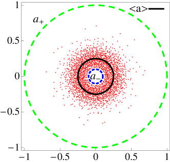
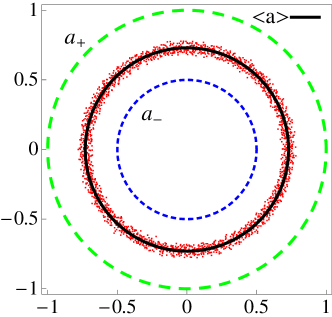
Figure 1. Spectrum of $M_{h}(a,\kappa)$ in the complex plane for $h^{-1}=2100$. The dashed circles correspond to $a_{+}$ and $a_{-}$, while the plain circle has radius $\langle a\rangle$. To the left, we plot $a=a_{1}$, and $a=a_{2}$ to the right.

For the damping terms, we choose two symbols of the form $a(q)$, whose quantizations are then diagonal matrices with entries $a(hj)$, $j=1,...,h^{-1}$. The function $a_{1}(q)$ has a plateau $a_{1}(q)=1$ for $q\in[1/3,2/3]$, another one for $q\in[0,1/6]\cup[5/6,1]$ and varies smoothly inbetween. For the second one, we take $a_{2}(q)=1-\frac{1}{2}\sin(2\pi q)^{2}$. Numerically, we have computed

$$\langle a_{1}\rangle\approx 0.250\,\quad\textrm{and}\quad\langle a_{2}\rangle\approx 0.728\,.$$

Fig. 1 and 2 represent the spectrum of our perturbed cat map for $h^{-1}=2100$, with dampings $a_{1}$ and $a_{2}$. The spectrum stay inside an anulus delimited by $a_{i+}$ and $a_{i-}$, as stated in Eq. (2.14), and the clustering of the eigenvalues around $\langle a\rangle_{i}$ is remarkable. For a more quantitative observation, the integrated radial and angular density of eigenvalues for different values of $h^{-1}$ are represented in Fig. 1. We check that for moduli, the curve jumps around $\langle a\rangle$, which denotes a maximal density around this value, and we clearly see the homogeneous angular repartition of the eigenvalues of $M_{h}(a,\kappa)$.

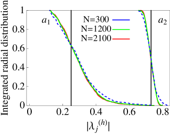
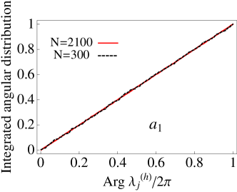
Figure 2. Integrated spectral densities for the perturbed cat map. The radial distribution is represented to the left, the vertical bars indicate the value $\langle a\rangle$ for $a=a_{1}$ and $a=a_{2}$. The angular distribution is represented to the right for the map $M_{h}(a_{1},\kappa)$.

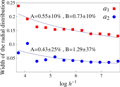
Figure 3. Width of the radial distribution, together with the best 2-parameter fits $A(\log h^{-1})^{-B}$ and the asymptotic standard errors.

As we can observe in Fig. 2, the width of the jumps do not depend a lot upon $h$, at least for the numerical range we have explored. This behavior could be explained by Theorem 1.3, which states that the speed of the clustering may be governed by $\log h^{-1}$. To check this observation more in detail, we define the width $W_{h}$ of the spectral distribution of $M_{h}(a,\kappa)$ as

$$W_{h}=|\lambda^{(h)}_{E(\frac{1}{4h})}|-|\lambda^{(h)}_{E(\frac{3}{4h})}|\,,$$

and plot $W_{h}$ as a function of $h$ – see Fig. 3. We clearly observe a decay with $h^{-1}$, although the 2-parameter fits $A(\log h^{-1})^{-B}$ hints a decay slightly faster than $(\log h^{-1})^{-1/2}$. Other numerical investigations presented in [NS] for the quantum baker map show the same type of decay, and a solvable quantization of the baker map allow to compute explicitely the width $W_{h}$, which turns to be exactly proportional to $\sqrt{\log h^{-1}}$. This result, together with the numerics presented above, seems to indicate that the bound on the decay of the eigenvalue distribution expressed by Theorem 1.3 may be optimal.

References

• [Ana] N. Anantharaman, workshop “Spectrum and dynamics”, Centre de Recherche Mathématiques, Montréal, April 7-11, 2008.
• [AL] M. Asch and G. Lebeau, The spectrum of the damped wave operator for a bounded domain in ${\mathbb{R}}^{2}$, Experimental math. 12 (2003), 227–241
• [AA] V.I. Arnold and A. Avez, “Ergodic problems of classical mechanics”, Addison-Wesley, 1968.
• [BK] P.A. Boasman and J.P. Keating, Semiclassical asymptotics of perturbed cat maps, Proc. R. Soc. Math. & Phys. Sc. 449 no. 1937, 629–653
• [BU] D. Borthwick and A. Uribe, On the pseudospectra of Berezin-Toeplitz operators, Meth. Appl. Anal. 10 (2003), 31–65
• [BDB1] A. Bouzouina and S. De Bièvre, Equipartition of the eigenfunctions of quantized ergodic maps on the torus, Commun. Math. Phys. 178 (1996), 83–105
• [BDB2] A. Bouzouina and S. De Bièvre, Équidistribution des valeurs propres et ergodicité semi-classique de symplectomorphismes du tore quantifiés, C. R. Acad. Sci. Paris Série I, 326 (1998), 1021–1024
• [BR] A. Bouzouina and D. Robert, Uniform semiclassical estimates for the propagation of quantum observables, Duke Math. Journal, 111 no. 2 (2002), 223-252
• [Com] L. Comtet, Analyse combinatoire, Vol. 1, Collection SUP: “Le Mathématicien” 4, Presses Univ. France, Paris, 1970. MR 41:6697
• [DEG] M. Degli Esposti and S. Graffi (eds): The mathematical aspects of quantum maps, Springer, 2003.
• [DS] M. Dimassi and J. Sjöstrand, Spectral Asymptotics in the semi-classical limit, Cambridge University Press, 1999.
• [ET] M. Embree and L.N. Trefethen, Spectra and pseudospectra, the behaviour of non-normal matrices and operators, Princeton Univ. Press, 2005.
• [FNW] A. Fannjiang, S. Nonnenmacher and L. Wolowski, Relaxation time for quantized toral maps, Annales Henri Poincar 7 no. 1 (2006), 161-198.
• [GS] A. Grigis and J. Sjöstrand, Microlocal analysis for differential operators, London math. soc. L.N.S. 196, Cambridge University Press (1983)
• [HB] J.H. Hannay and M.V. Berry: Quantization of linear maps on a torus - Fresnel diffraction by a periodic grating, Physica D1 (1980), 267–290
• [KMR] J.P. Keating, F. Mezzadri and J.M. Robbins: Quantum boundary conditions for torus maps. Nonlinearity 12 (1991), 579-591
• [KNS] J.P. Keating, M. Novaes, H. Schomerus: Model for chaotic dielectric microresonators, Phys. Rev. A 77 (2008), 013834.
• [Kön] H. König, Eigenvalues distribution for compact operators, Birkhäuser, 1986.
• [Liv] C. Liverani, Decay of correlations, Ann. of Math. 142 (1995), 239–301
• [MOK] J. Markolf and S. O’Keefe: Weyl’s law and quantum ergodicity for maps with divided phase space. Nonlinearity 18 (2005), 277–304
• [NS] S. Nonnenmacher and E. Schenck, arXiv:0803.1075v2 [nlin.CD] (2008), to appear in Phys. Rev. E.
• [NZ] S. Nonnenmacher and M. Zworski: Distribution of resonances for open quantum maps. Commun. Math. Phys. 269 (2007), 311–365
• [OP] S. Orey and S. Pelikan, Deviations of Trajectories Averages and the defect in Pesin’s Formula for Anosov Diffeomorphisms, Trans. Amer. Math. Soc. 315 no. 2 (1989), 741–753
• [RBY] L. Rey-Bellet and L.-S. Young, Large deviations in non-uniformly hyperbolic dynamical systems, Erg. Th. & Dynam. Sys. 28 (2008), 587–612
• [Rud] W. Rudin, Functional Analysis, McGraw-Hill, 1991.
• [Sjö] J. Sjöstrand, Asymptotic distribution of eigenfrequencies for damped wave equations, Publ. R.I.M.S. 36 (2000), 573–611
• [SZ] J. Sjöstrand and M. Zworski, Fractal upper bound on the density of semiclassical resonances, Duke Math. J. 137 no. 3 (2007), 381–459
• [Tab] M. Tabor, A semiclassical quantization of area-preserving maps, Physica D6 (1983), 195–210
• [Zel] S. Zelditch: Index and dynamics of quantized contact transformations. Annales de l’institut Fourier, 47 no. 1 (1997), 305–363
Acknowledgment
I would like to thank very sincerely St phane Nonnenmacher for suggesting this problem, and above all for his generous help and patience while introducing me to the subject. I also have benefitted from his careful reading of preliminary versions of this work. I would also like to thank Fr d ric Faure and Maciej Zworski for helpful and enlightening discussions.