Resolvents of $\mathscr{R}$-Diagonal Operators

Abstract.

We consider the resolvent $(\lambda-a)^{-1}$ of any $\mathscr{R}$-diagonal operator $a$ in a $\mathrm{II}_{1}$-factor. Our main theorem (Theorem 1.1) gives a universal asymptotic formula for the norm of such a resolvent. En route to its proof, we calculate the $\mathscr{R}$-transform of the operator $|\lambda-c|^{2}$ where $c$ is Voiculescu’s circular operator, and give an asymptotic formula for the negative moments of $|\lambda-a|^{2}$ for any $\mathscr{R}$-diagonal $a$. We use a mixture of complex analytic and combinatorial techniques, each giving finer information where the other can give only coarse detail. In particular, we introduce partition structure diagrams in Section 4, a new combinatorial structure arising in free probability.

1. Introduction

1.1. Motivation and Main Results

In this paper, we develop a number of universal norm estimates related to free probability theory. We are, in particular, concerned with $\mathscr{R}$-diagonal operators, which are precisely defined on page 1.2. Originally introduced by Nica and Speicher in [13], they have been considered by many authors in papers including [3, 4, 5, 6, 8, 10, 11, 12, 14, 17]. The class of $\mathscr{R}$-diagonal operators includes both Voiculescu’s circular operator and Haar unitary operators, and is very large (the distribution of the real part of an $\mathscr{R}$-diagonal operator can be prescribed arbitrarily). They are important in recent work on the invariant subspace conjecture relative to a $\mathrm{II}_{1}$-factor (cf. [5, 6], and have been shown to maximize free entropy given distribution constraints.

This paper is, in a sense, a continuation of [10] and [8], which examined an important norm inequality (the Haagerup inequality, [2]), originally in the context of Haar unitary operators, generalized to all $\mathscr{R}$-diagonal elements. The Haagerup inequality compares operator norm to $L^{2}$-norm for homogeneous (non-commutative) polynomials in operators. In [8], the second author considered an alternate formulation based on the dilation $a\mapsto ra$ for $r\in(0,1)$, acting on the $C^{\ast}$-algebra generated by a family of free generators $a$. Of interest are the elements $1+ra+(ra)^{2}+\cdots=(1-ra)^{-1}$. In that context, he proved a non-sharp version of the lower-bound in Theorem 1.1 below, for a sub-class of $\mathscr{R}$-diagonal operators (those with non-negative free cumulants). The current paper can be viewed as providing the sharp norm inequality, for all $\mathscr{R}$-diagonal operators.

Our main theorem, Theorem 1.1, gives the precise rate of norm blow-up of the resolvent of an $\mathscr{R}$-diagonal operator near its spectral radius. It is worthy of note for two reasons. First, it is notoriously difficult to calculate resolvent blow-up rates, while we have calculated the rate for all $\mathscr{R}$-diagonal resolvents. Second, the result is universal: the rate is always polynomial with exponent $-3/2$, and the constant is a product of a uniform factor with a quantity determined only by the $4th$ moment of the operator $a$.

Theorem 1.1.

Let $a$ be an $\mathscr{R}$-diagonal operator in a $\mathrm{II}_{1}$ factor $\mathscr{A}$ with trace $\varphi$, normalized so that $\varphi(aa^{\ast})=\|a\|_{2}^{2}=1$. Set $v(a)=\|a\|_{4}^{4}-1$. Then $v(a)>0$ iff $a$ is not a Haar unitary, and in this case, for $\lambda>1$,

$$\|(\lambda-a)^{-1}\|\sim\sqrt{\frac{27}{32}}\,\sqrt{v(a)}\,\frac{1}{(\lambda-1)^{3/2}}\quad\text{as}\quad\lambda\downarrow 1.$$ (1.1)

In proving Theorem 1.1, we develop several auxiliary results of independent interest. The special case that $a$ is Voiculescu’s circular element $c$ affords an example where non-asymptotic calculations may be done completely explicitly. In that case, we prove the following result on page 2.1, which (as we show) can be used to prove this special case of the main theorem.

Theorem 2.2.

Let $c$ be a circular operator of unit variance, and let $\lambda\in\mathbb{R}$. Then

$$\mathscr{R}_{|\lambda-c|^{2}}(z)=\frac{1}{1-z}+\frac{\lambda^{2}}{(1-z)^{2}}.$$

Theorem 2.2 is proved following its statement via combinatorial techniques; we reprove it in Section 3.1 using the analytic techniques developed there. We go on to use that analysis to calculate, to leading order, the negative moments of the operator $|\lambda-a|^{2}$ for any $\mathscr{R}$-diagonal $a$. The result, which appears on page 3.3, follows.

Theorem 3.11.

Let $k$ be a non-negative integer, and let $a$ satisfy the conditions of Theorem 1.1. Then as $\lambda\downarrow 1$,

$$\varphi(|\lambda-a|^{-2(k+1)})\sim C^{(2)}_{k}\frac{v(a)^{k}}{(\lambda^{2}-1)^{3k+1}},$$

where $C^{(2)}_{k}=\frac{1}{2k+1}\binom{3k}{k}$ are the (type $2$) Fuss-Catalan numbers.

We give two different proofs of this theorem: one complex analytic, in Section 3, and the other combinatorial, in Section 4.1. Theorem 3.11 by itself yields the sharp lower bound of Theorem 1.1, as detailed in Section 4.2; the analytic techniques of Section 3 extend to prove this bound is also sharp from above. In addition, our combinatorial approach demonstrates that the negative moments are in fact polynomials in appropriate quantities. The theorem, appearing on page 4.1, is as follows.

Theorem 4.8.

Let $k\geq 0$, and let $a$ satisfy the conditions of Theorem 1.1. Then there is a polynomial $P_{k+1}^{a}$ in two variables so that

$$\varphi(|\lambda-a|^{-2(k+1)})=P_{k+1}^{a}\left(\frac{1}{\lambda^{2}-1},\frac{1}{\lambda^{2}}\right).$$

for $\lambda>1$.

The proof of Theorem 4.8 led to the development of a new class of combinatorial objects we call partition structure diagrams, introduced in Section 4.1.

1.2. Background

Following is a brief description of those results and techniques from both the complex analytic and combinatorial sides of free probability theory that we use in this paper. They are here largely as a means to fix notation. The reader is directed to the papers [4, 5, 8, 10] and the book [15] for further reading.

The arena for all of what follows is a $\mathrm{II}_{1}$-factor $\mathscr{A}$ with trace $\varphi$. Operators in $\mathscr{A}$ are non-commutative random variables. If $x\in\mathscr{A}$ is self-adjoint, it has a spectral resolution $E^{x}$ whose projections are in $\mathscr{A}$; the measure $\mu_{x}=\varphi\circ E^{x}$ is the distribution or spectral measure of $x$. Equivalently, $\mu_{x}$ is the unique probability measure on $\mathbb{R}$ whose moments $\int t^{n}\,\mu_{x}(dt)$ are given by the moments $\varphi(x^{n})$ for $n\in\mathbb{N}$. Even if $x\in\mathscr{A}$ is not self-adjoint, we therefore refer to the collection of all $\varphi$-moments of monomials in $x$ and $x^{\ast}$ as the distribution of $x$.

Given a probability measure $\mu$ on $\mathbb{R}$, its Cauchy transform $G_{\mu}$ is the analytic function defined in the upper half-plane $\mathbb{C}_{+}$ by

$$G_{\mu}(z)=\int_{\mathbb{R}}\frac{1}{z-t}\,\mu(dt),\quad z\in\mathbb{C}_{+}.$$ (1.2)

The $\mathscr{R}$-transform of the measure, $\mathscr{R}_{\mu}$, is the analytic function defined in a neighbourhood of $0$ determined by the functional equation

$$G_{\mu}(\mathscr{R}_{\mu}(z)+1/z)=z,\quad z\in\mathbb{C}_{+},\quad|z|\text{ small}.$$ (1.3)

For a known $\mathscr{R}$-transform $\mathscr{R}_{\mu}$, Equation 1.3 in fact determines $G_{\mu}$ on a sector in $\mathbb{C}_{+}$, and thence on all of $\mathbb{C}_{+}$ by analytic continuation, modulo the asymptotic restriction that $\lim_{|z|\to\infty}zG_{\mu}(z)=1$. This relationship shows that the measure $\mu$ can be recovered from its $\mathscr{R}$-transform, via the Stieltjes inversion formula:

$$\mu(dt)=-\frac{1}{\pi}\lim_{\epsilon\downarrow 0}\Im G_{\mu}(t+i\epsilon)\,dt.$$ (1.4)

Equation 1.4 should be interpreted in weak form (that $\int f(t)\,\mu(dt)=-\frac{1}{\pi}\lim_{\epsilon\downarrow 0}\int f(t)\Im G_{\mu}(t+i\epsilon)\,dt$ for $f\in C_{c}(\mathbb{R})$) in general, but in the case that $\mu$ has a density $\rho$ with respect to Lebesgue measure $\mu(dt)=\rho(t)\,dt$, Equation 1.4 yields $\rho(t)$ as the limit on the right-hand-side.

Given $x,y\in\mathscr{A}$ self-adjoint, they are called free if $\mathscr{R}_{\mu_{x+y}}=\mathscr{R}_{\mu_{x}}+\mathscr{R}_{\mu_{y}}$. Freeness can be written in other more combinatorial forms by considering the additivity of $\mathscr{R}$-transforms as a collection of statements about Taylor coefficients. It is easy to verify that $\mathscr{R}_{\mu}(0)=0$ for any measure $\mu$, and so in general we have

$$\mathscr{R}_{\mu}(z)=\kappa_{1}(\mu)+\kappa_{2}(\mu)\,z+\kappa_{3}(\mu)\,z^{2}+\cdots$$

for some scalars $\kappa_{n}(\mu)$ called the free cumulants of $\mu$. Thinking of $\mathscr{R}$ and $\kappa_{n}$ indexed by a random variable rather than its distribution, we can polarize and express $\kappa_{n}$ as an $n$-linear functional: $\kappa_{n}[x_{1},\ldots,x_{n}]$, where $\kappa_{n}[x,\ldots,x]=\kappa_{n}(\mu_{x})$. In this language, freeness can be stated thus: random variables are free if all their mixed free cumulants vanish. This parallels the classical connection between independence of random variables and their classical cumulants (also known as semi-invariants). It also provides an extension of the notion of freeness to any collection of (not necessarily self-adjoint) random variables.

The relationship between moments and free cumulants is given by the moment cumulant formula:

$$\varphi(x_{1}\cdots x_{n})=\sum_{\pi\in NC(n)}\kappa_{\pi}[x_{1},\ldots,x_{n}].$$ (1.5)

Here $NC(n)$ denotes the lattice of non-crossing partitions of the ordered set $\{1,\ldots,n\}$. Given a partition $\pi=\{B_{1},\ldots,B_{r}\}$ (with $B_{j}\subseteq\{1,\ldots,n\}$), the quantity $\kappa_{\pi}[x_{1},\ldots,x_{n}]$ is equal to the product of the $r$ terms $\kappa(B_{j})[x_{1},\ldots,x_{n}]$, where if $B=\{i_{1},\ldots,i_{m}\}$ then $\kappa(B)[x_{1},\ldots,x_{n}]=\kappa_{m}[x_{i_{1}},\ldots,x_{i_{m}}]$. For example, if $\pi=\left\{\{1,4,5\},\{2,3\}\right\}$, then $\kappa_{\pi}[x_{1},\ldots,x_{5}]=\kappa_{3}[x_{1},x_{4},x_{5}]\,\kappa_{2}[x_{2},x_{3}]$.

An non-commutative random variable $a\in\mathscr{A}$ is called $\mathscr{R}$-diagonal if, among all mixed free cumulants in $a,a^{\ast}$, the only non-zero ones are among

$$\kappa_{2n}[a,a^{\ast},\ldots,a,a^{\ast}],\quad\kappa_{2n}[a^{\ast},a,\ldots,a^{\ast},a],$$

for some positive integer $n$. Prominent examples of $\mathscr{R}$-diagonal operators are Haar unitary operators and Voiculescu’s circular operator $c$, often represented in the form $c=\frac{1}{\sqrt{2}}(s+is^{\prime})$ where $s,s^{\prime}$ are free semicircular random variables — self-adjoint operators with distribution $\mu_{s}(dt)=\mu_{s^{\prime}}(dt)=\frac{1}{2\pi}\sqrt{4-t^{2}}\mathbbm{1}_{\{|t|\leq 2\}}$). The class of $\mathscr{R}$-diagonal operators is closed under free sum and product and taking powers, and for any compactly-supported probability measure $\mu$ on $\mathbb{R}_{+}$ there is an $\mathscr{R}$-diagonal operator $a$ with $\mu_{aa^{\ast}}=\mu$.

The general moment–cumulant formula takes a special form in the case of $\mathscr{R}$-diagonal operators. Let $a$ be $\mathscr{R}$-diagonal, and consider any monomial in $a,a^{\ast}$: $a^{\ast n_{1}}a^{m_{1}}\cdots a^{\ast n_{k}}a^{m_{k}}$ for $n_{1},\ldots,m_{k}$ non-negative integers. The following formula is a consequence of the definition of $\mathscr{R}$-diagonality, and is proved in [8].

$$\varphi(a^{\ast n_{1}}a^{m_{1}}\cdots a^{\ast n_{k}}a^{m_{k}})=\sum_{\pi\in NC(n_{1},m_{1},\ldots,n_{k},m_{k})}\kappa_{\pi}[a^{,n_{1}},a^{\ast,m_{1}},\ldots,a^{,n_{k}},a^{\ast,m_{k}}].$$ (1.6)

Here $NC(n_{1},m_{2},\ldots,n_{k},m_{k})$ denotes the set of non-crossing partitions $\pi$ of the list of length $n_{1}+m_{1}+\cdots+n_{k}+m_{k}$ with the property that each block of $\pi$ alternately connects $a$s and $a^{\ast}$s. Commas have been added in the exponents of the cumulants to emphasize that the arguments are not products. The set of pairings with this property is denoted $NC_{2}(n_{1},m_{1},\ldots,n_{k},m_{k})$.

Figure 1. Two non-crossing partitions in $NC(2,3,4,3)$, represented in linear format (top) and on the disc (bottom); the latter representation will be more useful in Section 4.1. The first partition is a pairing in $NC_{2}(2,3,4,3)$.

In fact, it is sometimes useful to consider cumulants with products as arguments (thus the need for the commas above to distinguish). The following theorem (Theorem 11.12 in [15]) is a powerful computational tool we will use in Section 2.

Theorem 1.2.

Let $\mathbf{i}=(i_{1},\ldots,i_{n})$ be an $n$-tuple of natural numbers, and let $a_{1},\ldots,a_{|\mathbf{i}|}$ be random variables in a non-commutative probability space. Consider the products

$$A_{1}=a_{1}\cdots a_{i_{1}}\quad A_{2}=a_{i_{1}+1}\cdots a_{i_{1}+i_{2}}\quad\ldots\quad A_{n}=a_{i_{1}+\cdots+i_{n-1}+1}\cdots a_{i_{1}+\cdots+i_{n}}.$$

The free cumulants of these product variables are given in terms of the free cumulants of the $a_{j}$ themselves by

$$\kappa_{n}[A_{1},\ldots,A_{n}]=\sum_{\pi\in NC(|\mathbf{i}|)\atop\pi\vee\widehat{0_{n}}=1_{|\mathbf{i}|}}\kappa_{\pi}[a_{1},\ldots,a_{|\mathbf{i}|}],$$ (1.7)

where $\widehat{0_{n}}$ is the partition whose blocks are the intervals $\{1,\ldots,i_{1}\},\{i_{1}+1,\ldots,i_{1}+i_{2}\},\ldots,\{i_{1}+\cdots+i_{n-1}+1,\ldots,i_{1}+\cdots+i_{n}\}$.

Remark 1.3.

For notational convenience, we will express the relationship between the tuples $\mathbf{A}=[A_{1},\ldots,A_{n}]$ and $\mathbf{a}=[a_{1},\ldots,a_{\mathbf{i}}]$ in Equation 1.7 by $\mathbf{a}=\widehat{\mathbf{A}}$. For example, if $\mathbf{i}=(2,1,2,1)$ then $\mathbf{A}=[a_{1}a_{2},a_{3},a_{4}a_{5},a_{6}]$ and so $\widehat{\mathbf{A}}=[a_{1},a_{2},a_{3},a_{4},a_{5},a_{6}]$. The use of the notation is in summations over $\mathbf{i}$, where it is cumbersome to explicitly enumerate the break-points between products.

The $\vee$ in Equation 1.7 denotes the join in the lattice $NC(|\mathbf{i}|)$. The meaning of the condition $\pi\vee\widehat{0_{n}}=1_{|\mathbf{i}|}$ is as follows: the blocks of $\pi$ must connect the blocks of $\widehat{0_{n}}$. To be precise: given any two points $p,q$ in $\{1,\ldots,|\mathbf{i}|\}$, there must be a path $p=p_{1}\sim_{\sigma_{1}}p_{2}\sim_{\sigma_{2}}\cdots\sim_{\sigma_{r-1}}p_{r}=q$ where $\sigma_{j}\in\{\pi,\widehat{0_{n}}\}$ for $j=1\ldots r-1$. Indeed, the sequence $\sigma_{j}$ can be chosen to alternate between $\pi$ and $\widehat{0_{n}}$. Figure 2 gives examples.

Figure 2. Three examples of partitions in $NC(6)$. With multi-index $\mathbf{i}=(2,1,2,1)$, $\pi_{1}$ and $\pi_{2}$ do connect all the blocks of $\widehat{0_{4}}$, and so would be included in the sum in Equation 1.7; $\pi_{3}$ leaves the first block of $\widehat{0_{4}}$ isolated, and so is not included in this sum.

1.3. Organization

This paper is organized as follows. In Section 2, we address our main theorem through the special case of a circular operator $c$, the pre-eminent example of an $\mathscr{R}$-diagonal element. In Section 2.1, we calculate the $\mathscr{R}$-transform of the operator $|\lambda-c|^{2}$ for any scalar $\lambda$, using combinatorial means (primarily judicious application of Theorem 1.2). In Section 2.2, we us this $\mathscr{R}$-transform to explicitly determine the support of the spectral measure of $|\lambda-c|^{2}$; its left boundary point represents the norm of the resolvent $(\lambda-c)^{-1}$. In this case, the measure itself can be completely determined.

The exact calculations of Section 2.2 cannot be extended to the general $\mathscr{R}$-diagonal case, and so we proceed to develop analytic arguments to prove the asymptotic statement of Theorem 1.1. In Section 3, we demonstrate the power of working with the symmetrizations of spectral measures (via Equations 3.2 and 3.3). Section 3.1 shows how Theorem 2.2 can be obtained directly from these analytic means. Section 3.2 gives a general analytic continuation argument from the above-mentioned equations that yields a useful power-series inversion formula, which is then used in Section 3.3 to calculate (to leading order) the negative absolute moments of the resolvent $(\lambda-a)^{-1}$ (theorem 3.11). These techniques are then pushed through to give a complete proof of Theorem 1.1 in Section 3.4.

Finally, in Section 4, we examine the combinatorial structures underlying the negative absolute moments of the resolvent $(\lambda-a)^{-1}$. In Section 4.1, we introduce partition structure diagrams, a new way to view the basic structure of partitions appearing in Equation 1.6 for $\mathscr{R}$-diagonal operators, and use their enumeration to provide a bijective combinatorial proof of the refinement (Theorem 4.8) of Theorem 3.11. Then, in Section 4.2, we show how knowledge of the asymptotics of negative moments alone can be used to recapture the sharp lower-bound of Theorem 1.1.

2. The Circular Case

Let $c$ be a circular operator of unit variance in a $\mathrm{II}_{1}$-factor $\mathscr{C}$. Since $c$ is $\mathscr{R}$-diagonal, its spectral radius is $\|c\|_{2}=1$ by our choice of variance. Hence the resolvent

$$R_{c}(\lambda)=(\lambda-c)^{-1}$$

is a $\mathscr{C}$-valued analytic function on the domain $|\lambda|>1$. Our goal in this section is to calculate $\|R_{c}(\lambda)\|$ to leading order as $|\lambda|\downarrow 1$.

Remark 2.1.

Note that $c$ is rotationally-invariant; it follows that if $\theta\in\mathbb{R}$ then $\|R_{c}(\lambda e^{-i\theta})\|=\|R_{c}(\lambda)\|$. Hence, we restrict our attention to the case $\lambda>1$ in $\mathbb{R}$.

For $\lambda>1$, define the positive operator $T_{\lambda}$ by

$$T=T_{\lambda}=R_{c}(\lambda)^{\ast}R_{c}(\lambda)=(\lambda-c^{\ast})^{-1}(\lambda-c)^{-1}.$$ (2.1)

Note that $\|R_{c}(\lambda)\|^{2}=\|T_{\lambda}\|$. What’s more, since $T>0$ it follows that $\|T\|=\inf\mathrm{spec}\,(T^{-1})$, and $T^{-1}=(\lambda-c)(\lambda-c^{\ast})=|\lambda-c|^{2}$ is an operator we can handle with combinatorial techniques. In particular, we will now calculate the $\mathscr{R}$-transform of this operator, which will allow us to calculate the spectral measure of $T^{-1}$ through Equations 1.2 and 1.3.

2.1. The $\mathscr{R}$-transform of $|\lambda-c|^{2}$

Theorem 2.2.

Let $c$ be a circular operator of unit variance, and let $\lambda\in\mathbb{R}$. Then

$$\mathscr{R}_{|\lambda-c|^{2}}(z)=\frac{1}{1-z}+\frac{\lambda^{2}}{(1-z)^{2}}.$$ (2.2)

Remark 2.3.

We find the formula in Equation 2.2 interesting in its own right. It mirrors a similar formula for the semicircular equivalent provided in [7]; if $s$ is a semicircular operator of variance $1$,

$$\mathscr{R}_{(\lambda-s)^{2}}(z)=\frac{1}{1-z}+\frac{\lambda^{2}}{(1-2z)^{2}}.$$

Their techniques are entirely analytic: indeed, one can calculate the Cauchy-transform of $(\lambda-s)^{2}$ from that of $\lambda-s$, the latter of which is well-known, and then the $\mathscr{R}$-transform is achieved through Equation 1.3. Our approach below is markedly different, using only combinatorial techniques; however, analytic techniques will be developed to study the more general case in later sections, and we will rederive Equation 2.2 using those techniques in Section 3.1

Proof.

Expand $|\lambda-c|^{2}=\lambda^{2}-\lambda(c+c^{\ast})+cc^{\ast}$. Denote $\alpha_{1}=-\lambda(c+c^{\ast})$ and $\alpha_{2}=cc^{\ast}$, so that $|\lambda-c|^{2}=\lambda^{2}+\alpha_{1}+\alpha_{2}$. The constant $\lambda^{2}$ is free from any operator, and so we have an initial simplification

$$\mathscr{R}_{|\lambda-c|^{2}}(z)=\mathscr{R}_{\lambda^{2}}(z)+\mathscr{R}_{\alpha_{1}+\alpha_{2}}(z)=\lambda^{2}+\mathscr{R}_{\alpha_{1}+\alpha_{2}}(z).$$ (2.3)

Now, $\alpha_{1},\alpha_{2}$ are certainly not free. We calculate the $\mathscr{R}$-transform of their sum as a power-series whose coefficients are free cumulants:

$$\mathscr{R}_{\alpha_{1}+\alpha_{2}}(z)=\sum_{n\geq 1}\kappa_{n}[\alpha_{1}+\alpha_{2},\ldots,\alpha_{1}+\alpha_{2}]\,z^{n-1}.$$ (2.4)

The free cumulant $\kappa_{n}$ is a multilinear function, and so we can expand

$$\kappa_{n}[\alpha_{1}+\alpha_{2},\ldots,\alpha_{1}+\alpha_{2}]=\sum_{(i_{1},\ldots,i_{n})\in\{1,2\}^{n}}\kappa_{n}[\alpha_{i_{1}},\ldots,\alpha_{i_{n}}].$$ (2.5)

We will shortly see that the vast majority of the $2^{n}$ terms in the sum in Equation 2.5 are $0$. To ease notation, let $\mathbf{i}$ denote the multi-index $(i_{1},\ldots,i_{n})$, and denote the $n$-tuple $\alpha_{i_{1}},\ldots,\alpha_{i_{n}}$ as $\alpha_{\mathbf{i}}$. Since $\alpha_{2}=cc^{\ast}$ is a product, for each $\mathbf{i}$ we can expand the cumulant in Equation 2.5 using Equation 1.7.

$$\kappa_{n}[\alpha_{\mathbf{i}}]=\sum_{\pi\in NC(|\mathbf{i}|)\atop\pi\vee\widehat{0_{n}}=1_{|\mathbf{i}|}}\kappa_{\pi}[\widehat{\alpha_{\mathbf{i}}}].$$ (2.6)

As in Remark 1.3, the list $\widehat{\alpha_{\mathbf{i}}}$ is the expanded list of products from $\alpha_{\mathbf{i}}$. For example, if $\mathbf{i}=(2,1,2,1)$ so that $\alpha_{\mathbf{i}}=[\alpha_{2},\alpha_{1},\alpha_{2},\alpha_{1}]=[cc^{\ast},\alpha_{1},cc^{\ast},\alpha_{1}]$, then $\widehat{\alpha_{\mathbf{i}}}=[c,c^{\ast},\alpha_{1},c,c^{\ast},\alpha_{1}]$.

Since $\alpha_{1}=-\lambda(c+c^{\ast})$, any such cumulant $k_{\pi}[\widehat{\alpha_{\mathbf{i}}}]$ can be expanded into a sum of cumulants $k_{\pi}$ of a list of $c$s and $c^{\ast}$s. Since the only non-vanishing block $\ast$-cumulants of $c$ are $\kappa_{2}[c,c^{\ast}]=\kappa_{2}[c^{\ast},c]=1$, this means that the only $\pi$ which can contribute to the sum 2.6 are non-crossing pairings. This turns out to be an enormous simplification of the sum 2.5; the result is most of these terms are $0$. Let us first consider the two endpoints.

Suppose $\mathbf{i}=(1,1,\ldots,1)$. The corresponding term in Equation 2.5 is

$$\kappa_{n}[\alpha_{1},\ldots,\alpha_{1}]=(-\lambda)^{n}\kappa_{n}[c+c^{\ast},\ldots,c+c^{\ast}].$$

Expanding this in $2^{n}$ terms, we have mixed cumulants in $c,c^{\ast}$, only two of which are non-vanishing: $\kappa_{2}[c,c^{\ast}]=\kappa_{2}[c^{\ast},c]=1$. Hence,

$$\kappa_{n}[\alpha_{1},\ldots,\alpha_{1}]=2\lambda^{2}\mathbbm{1}_{\{n=2\}}.$$ (2.7)

On the other hand, suppose $\mathbf{i}=(2,2,\ldots,2)$. The corresponding term in Equation 2.5 is

$$\kappa_{n}[\alpha_{2},\ldots,\alpha_{2}]=\kappa_{n}[cc^{\ast},cc^{\ast},\ldots,cc^{\ast}].$$

Employing Theorem 1.2 and the above observation that only pairings contribute, we can expand this cumulant as a sum,

$$\kappa_{n}[cc^{\ast},\ldots,cc^{\ast}]=\sum_{\pi\in NC_{2}(2n)\atop\pi\vee\widehat{0_{n}}=1_{2n}}\kappa_{\pi}[c,c^{\ast},\ldots,c,c^{\ast}].$$ (2.8)

In this case, $\widehat{0_{n}}=\{\{1,2\},\{3,4\},\ldots,\{2n-1,2n\}\}$. Let $\pi$ be any pairing that connects these blocks, and consider the block in $\pi$ containing $1$. Since $\pi$ is non-crossing, the match to $1$ must be even (or there would be an odd number of points in between that could therefore not be paired in a non-crossing manner). Suppose $1\sim_{\pi}{2k}$. If $k<n$, then there can be no non-crossing path joining $2k+1$ to $2k$, since such a concatenation of pairings would have to cross the pairing $\{1,2k\}$, as demonstrated in Figure 3.

Figure 3.

Hence, it must be that $1\sim_{\pi}2n$. Now, consider the match to $2$: say $2\sim_{\pi}2\ell+1$. If $\ell>1$, then the point $3$ cannot be connected to $2$ with a path composed of blocks in $\pi$ and $\widehat{0_{n}}$: since $\pi$ is non-crossing, the match to $3$ must be either $4$ or lie within the blocks $\{5,6\},\ldots,\{2\ell-1,2\ell\}$. None of these blocks can be connected to any other blocks of $\widehat{0_{n}}$ via $\pi$ without crossing the pairing $\{2,2\ell+1\}$. Hence, it must be that $2\sim_{\pi}3$. This is demonstrated in Figure 4.

Figure 4.

Iterating this argument shows that, in fact, there is only one pairing $\pi\in NC_{2}(2n)$ for which $\pi\vee\widehat{0_{n}}=1_{2n}$: the pairing $\varpi_{n}=\{\{1,2n\},\{2,3\},\{3,4\},\ldots,\{2n-2,2n-1\}\}$ pictured in Figure 5.

Figure 5. The pairing $\varpi_{n}$ is the unique pairing for which $\varpi_{n}\vee\widehat{0_{n}}=1_{2n}$ where $\widehat{0_{n}}=\{\{1,2\},\{3,4\},\ldots,\{2n-1,2n\}\}$.

Hence, we have from Equation 2.8,

$$\kappa_{n}[\alpha_{2},\ldots,\alpha_{2}]=\kappa_{\varpi_{n}}[c,c^{\ast},\ldots,c,c^{\ast}]=\kappa_{2}[c,c^{\ast}]\kappa_{2}[c^{\ast},c]^{n-1}=1.$$ (2.9)

Now, we must consider the remaining $2^{n-1}$ terms in Equation 2.5, all incorporating some mixture of $\alpha_{1}$s and $\alpha_{2}$s. The following lemmas show that only $n$ of these terms are non-zero.

Lemma 2.4.

Suppose $\mathbf{i}$ is a length $n$ string containing both $1$s and $2$s, and let $\widehat{0_{n}}$ denote the corresponding interval partition. If there exists $\pi\in NC_{2}(|\mathbf{i}|)$ such that $\pi\vee\widehat{0_{n}}=1_{|\mathbf{i}|}$, then $\mathbf{i}$ contains precisely two $1$s.

For the proof of Lemma 2.4, note first that $|\mathbf{i}|=\#1$s in $\mathbf{i}+2\cdot\#2$s in $\mathbf{i}$, and so for there to be any pairings, the number of $1$s must be even. Suppose, then, that $u,v,w\in\{1,\ldots,|\mathbf{i}|\}$ are distinct elements at positions corresponding to $1$s in $\mathbf{i}$. The condition $\pi\vee\widehat{0_{n}}=1_{|\mathbf{i}|}$ implies that there are paths

$$v =u_{1}\sim_{\sigma_{1}}u_{2}\sim_{\sigma_{2}}\cdots\sim_{\sigma_{r-2}}u_{r-1}\sim_{\sigma_{r-1}}u_{r}=u,$$

$$v =w_{1}\sim_{\tau_{1}}w_{2}\sim_{\tau_{2}}\cdots\sim_{\tau_{s-2}}w_{s-1}\sim_{\tau_{s-1}}w_{s}=w,$$

where the sequences $\sigma_{j}$ and $\tau_{j}$ alternate between $\pi$ and $\widehat{0_{n}}$. By assumption, $v$ corresponds to a singleton in $\widehat{0_{n}}$, and so (assuming that the paths are “minimal” so that no number appears as two differently indexed $u_{j}$ or $v_{j}$) we must have $\sigma_{1}=\tau_{1}=\pi$. But $\pi$ is a pairing, so there is a unique point $v_{2}$ with $u_{1}=w_{1}\sim v_{2}$, and therefore $u_{2}=w_{2}=v_{2}$. Then $v_{2}\sim_{\sigma_{2}}u_{3}$ and $v_{2}\sim_{\tau_{2}}w_{3}$, where $\sigma_{2}=\tau_{2}=\widehat{0_{n}}$. If $v_{2}$ is a singleton in $\widehat{0_{n}}$, then this is the end of both paths, meaning $u=u_{2}=w_{2}=w$, contradicting our assumption. Otherwise, the block of $\widehat{0_{n}}$ containing $v_{2}$ is a $2$-block, in which case there is a unique $v_{3}$ with $v_{2}\sim_{\widehat{0_{n}}}v_{3}$, and so $u_{3}=w_{3}=v_{3}$. Continuing inductively, we reach a contradiction to the fact that $u\neq w$. Hence, there must be precisely two $1$s in $\mathbf{i}$.

Remark 2.5.

The above proof is really just the following trivial observation: the singletons in $\widehat{0_{n}}$ must be ends of a path joining blocks, and a path can have only $0$ or $2$ ends, thence $\widehat{0_{n}}$ can have only $0$ or $2$ $1$s if it is to have this path-connected property.

Lemma 2.4 shows that the only contributing $\mathbf{i}$ to Equation 2.5 are those of the form $2^{\epsilon_{1}}\,1\,2^{\epsilon_{2}}\,1\,2^{\epsilon_{3}}$ for some $\epsilon_{1},\epsilon_{2},\epsilon_{3}\geq 0$. The next Lemma shows that either $\epsilon_{2}=0$ or $\epsilon_{1}=\epsilon_{3}=0$ in order for the term to contribute.

Lemma 2.6.

Suppose $\mathbf{i}$ is a length $n$ string containing both $1$s and $2$s, and let $\widehat{0_{n}}$ denote the corresponding interval partition. If $\mathbf{i}$ contains the substring $(1,2,1,2)$ or $(2,1,2,1)$, then $\kappa_{n}[\alpha_{\mathbf{i}}]=0$.

For the proof of Lemma 2.6, note that the discussion following Equation 2.8 may be applied locally, and so in a string of the form $\mathbf{i}=2^{\epsilon_{1}}\,1\,2^{\epsilon_{2}}\,1\,2^{\epsilon_{3}}$ where $\epsilon_{1},\epsilon_{2},\epsilon_{3}>0$, any pairing $\pi$ that connects the blocks of $\widehat{0_{n}}$ must pair according to the dark lines of Figure 6.

Figure 6.

The two singletons cannot pair together, since they would then be isolated by $\widehat{0_{n}}$. There are thence four positions where the two singletons may pair. If the two singletons pair to the $\epsilon_{1}$ and $\epsilon_{3}$ blocks, then the $\epsilon_{2}$ block is isolated, hence at least one singleton must pair to the $\epsilon_{2}$ block, and then the other must pair outside the $\epsilon_{2}$ block (or again that block would be isolated). Without loss of generality, suppose that the first singleton pairs to the $\epsilon_{2}$ block (otherwise we could simply reflect the figure). It must therefore pair to the adjacent position (or else this position cannot pair anywhere without a crossing). The remaining singleton must pair to its adjacent block, $\epsilon_{3}$, for otherwise the right-most open slot in the $\epsilon_{2}$-block could not be paired without crossings. These pairings are represented in the light lines in Figure 6. This forces the remaining pairing in $\pi$ (between the right-most points in the $\epsilon_{1}$ and $\epsilon_{2}$ blocks) to match a $c^{\ast}$ with a $c^{\ast}$, resulting in a $0$ cumulant. Therefore, although this pairing does satisfy the connectedness condition $\pi\vee\widehat{0_{n}}=1_{|\mathbf{i}|}$, the cumulant $\kappa_{n}[\alpha_{|\mathbf{i}|}]=0$.

Hence, at least one of $\epsilon_{1},\epsilon_{2},\epsilon_{3}$ must be $0$. If either $\epsilon_{1}$ or $\epsilon_{3}$ is $0$ while the other two are $>0$, the above argument (unchanged) gives the same result. So consider the case that $\epsilon_{2}=0$ while $\epsilon_{1},\epsilon_{3}>0$, represented in Figure 7. The local argument above Figure 6 yields the necessity of the dark lines here.

Figure 7.

Since the two singletons cannot pair together (as that block would be isolated), there is only one non-crossing pairing, given by the light lines in Figure 7. Each of the dark lines gives a contribution $\kappa_{2}[c^{\ast},c]$ (or $\kappa_{2}[c,c^{\ast}]$ for the outside pairing), yielding $1$. The remaining pairings are $\kappa_{2}[c^{\ast},\alpha_{1}]$ and $\kappa_{2}[\alpha_{1},c]$. Hence, the index $\mathbf{i}=2^{\epsilon_{1}}\,1\,1\,2^{\epsilon_{3}}$ with $\epsilon_{1},\epsilon_{3}>0$ yields $\kappa_{n}[\alpha_{\mathbf{i}}]=\kappa_{2}[c^{\ast},\alpha_{1}]\cdot\kappa_{2}[\alpha_{1},c]$, which is non-zero (we calculate it below).

Finally, we consider the case that only one of $\epsilon_{1},\epsilon_{2},\epsilon_{3}$ is non-zero. (The case that all three vanish means that $n=2$, and we will consider that case separately at the end.) Each of these three cases is really just a rotation of the one non-zero contributing case above: that is, a cyclic permutation of the string $\mathbf{i}=2^{\epsilon_{1}}\,1\,1\,2^{\epsilon_{3}}$ already considered. There are a total of $n$ such permutations, and each contributes the same cumulant (this follows from the fact that cyclic permutations induce lattice-isomorphisms of $NC(|\mathbf{i}|)$). Hence, each of these $n$ contributes the term $\kappa_{2}[c^{\ast},\alpha_{1}]\cdot\kappa_{2}[\alpha_{1},c]$. This completes the proof of Lemma 2.6.

Let us now collect all terms contributing to Equation 2.5. For $n>2$, Equation 2.7 yields that if $\mathbf{i}$ contains only $1$s then there is no contribution to the $n$th cumulant, and Equation 2.9 gives a contribution of $1$ in the case that $\mathbf{i}$ contains only $2$s. Lemmas 2.4 and 2.6 then show that among all other $\mathbf{i}$, only $n$ contribute a non-zero cumulant, each equal to the product $\kappa_{2}[c^{\ast},\alpha_{1}]\cdot\kappa_{2}[\alpha_{1},c]$, which we now calculate:

$$\kappa_{2}[c^{\ast},\alpha_{1}] =\kappa_{2}[c^{\ast},-\lambda(c+c^{\ast})]=-\lambda\left(\kappa_{2}[c^{\ast},c]+\kappa_{2}[c^{\ast},c^{\ast}]\right)=-\lambda$$

$$\kappa_{2}[\alpha_{1},c] =\kappa_{2}[-\lambda(c+c^{\ast}),c]=-\lambda\left(\kappa_{2}[c,c]+\kappa_{2}[c^{\ast},c]\right)=-\lambda.$$

Hence, the total contribution is

$$\kappa_{n}[\alpha_{1}+\alpha_{2},\ldots,\alpha_{1}+\alpha_{2}]=1+n\lambda^{2},\quad n>2.$$ (2.10)

For $n=1$, $\kappa_{1}$ is the mean; $\kappa_{1}[c]=\kappa_{1}[c^{\ast}]=0$, and so $\kappa_{1}[\alpha_{1}+\alpha_{2}]=\kappa_{1}[cc^{\ast}]=1$. The second cumulant nearly fits into the above analysis, but can be handled separately more easly:

$$\kappa_{2}[\alpha_{1}+\alpha_{2},\alpha_{1}+\alpha_{2}]=\kappa_{2}[\alpha_{1},\alpha_{1}]+\kappa_{2}[\alpha_{1},\alpha_{2}]+\kappa_{2}[\alpha_{2},\alpha_{1}]+\kappa_{2}[\alpha_{2},\alpha_{2}].$$

The two middle terms are odd, and since odd cumulants of $c,c^{\ast}$ are $0$, these cumulants are $0$. The first and last terms are included in Equations 2.7 and 2.9, and yield $2\lambda^{2}$ and $1$, respectively. Thus, from Equation 2.4 we have

$$\mathscr{R}_{\alpha_{1}+\alpha_{2}}(z)=1+(1+2\lambda^{2})z+\sum_{n\geq 3}(1+n\lambda^{2})z^{n-1},$$

and so

$$\mathscr{R}_{|\lambda-c|^{2}}(z)=\lambda^{2}+1+(1+2\lambda^{2})z+\sum_{n\geq 3}(1+n\lambda^{2})z^{n-1}=\sum_{n\geq 1}(1+n\lambda^{2})z^{n-1},$$

yielding the power-series expansion of Equation 2.2 as required. ∎

2.2. The support of the spectral measure of $|\lambda-c|^{2}$

Denote by $K_{|\lambda-c|^{2}}$ the function

$$K_{|\lambda-c|^{2}}(z)=\mathscr{R}_{|\lambda-c|^{2}}(z)+1/z.$$

From Equation 1.3, $G_{\mu_{\lambda}}(K_{|\lambda-c|^{2}}(z))=z$ for small $z\in\mathbb{C}_{+}$, where $G_{\mu_{\lambda}}$ is the Cauchy transform of the spectral measure $\mu_{\lambda}$ of $|\lambda-c|^{2}$. The result of Theorem 2.2 yields

$$K_{|\lambda-c|^{2}}(z)=\frac{1}{z}+\frac{1}{1-z}+\frac{\lambda^{2}}{(1-z)^{2}}=\frac{1+(\lambda^{2}-1)z}{z(1-z)^{2}}.$$ (2.11)

For notational convenience, let

$$m=\lambda^{2}-1\qquad K_{m}\equiv K_{|\lambda-c|^{2}}\qquad G_{m}=G_{\mu_{\lambda}}.$$ (2.12)

So $G_{m}\circ K_{m}(z)=z$ for small $z\in\mathbb{C}_{+}$. Our goal is to determine the support of the measure $\mu_{\lambda}$. Note that this support set is precisely the set of singular points for the Cauchy transform $G_{m}$, which we now set out to determine. The first derivative of $K_{m}(z)$ is given by

$$K_{m}^{\prime}(z)=\frac{1-3z-2mz^{2}}{z^{2}(z-1)^{3}}.$$ (2.13)

The quadratic polynomial in the numerator has two zeroes,

$$z^{\pm}=\frac{-3\pm\sqrt{9+8m}}{4m}.$$

Since $m=\lambda^{2}-1>0$ it is easy to check that

$$z^{-}\in(-\infty,0)\quad\text{and}\quad z^{+}\in(0,1).$$

Moreover, by factoring the polynomial in the numerator of Equation 2.13, one has

$$K_{m}^{\prime}(z)=-\frac{2m(z-z^{-})(z-z^{+})}{z^{2}(z-1)^{3}}$$

which shows that

$$K_{m}^{\prime}(z)<0\quad\text{for}\quad z\in(z^{-},0)\cup(0,z^{+}).$$

Thus $K_{m}^{\prime}$ is a strictly decreasing function on each of the intervals $(z^{-},0)$ and $(0,z^{+})$. Now, set $s^{\pm}\equiv K_{m}(z^{\pm})$; then simple (though tedious) calculation yields

$$s^{\pm}=\frac{27+36m+8m^{2}\pm(9+8m)^{3/2}}{8(m+1)}.$$ (2.14)

Since $\lim_{z\to 0\pm}K_{m}(z)=\pm\infty$, $K_{m}$ is a decreasing bijection of $(z^{-},0)$ onto $(-\infty,s^{-})$ and $K_{m}$ is also a decreasing bijection of $(0,z^{+})$ onto $(s^{+},\infty)$. Moreover since $s^{-}<s^{+}$ by Equation 2.14, $K_{m}$ is a bijection of $(z^{-},0)\cup(0,z^{+})$ onto $(-\infty,s^{-})\cup(s^{+},\infty)$. Let

$$L_{m}\colon(-\infty,s^{-})\cup(s^{+},\infty)\to(z^{-},0)\cup(0,z^{+})$$

denote the (function) inverse of the above restriction of $K_{m}$. Then $L_{m}(w)=G_{m}(w)$ for large values of $|w|$. Moreover, $L_{m}$ is real analytic, and can therefore be extended to a complex analytic function $\tilde{L}_{m}$ in a complex neighbourhood $U$ of $(-\infty,s^{-})\cup(s^{+},\infty)$, which we can assume has only two connected components $U^{-}\supset(-\infty,s^{-})$ and $U^{+}\supset(s^{+}\infty)$. By uniqueness of analytic continuation to open connected sets, it follows that $\tilde{L}_{m}(w)=G_{m}(w)$ for all $w\in U$. In particular, $G_{m}$ has no singular points in $(-\infty,s^{-})\cup(s^{+},\infty)$. Ergo, it follows that

$$\mathrm{supp}\,\mu_{\lambda}\subseteq[s^{-},s^{+}].$$ (2.15)

Since $K_{m}^{\prime}(z^{\pm})=0$, the graph of $L_{m}$ has vertical tangents at the endpoints $(s^{-},z^{-})$ and $(s^{+},z^{+})$. Therefore $s^{\pm}$ are both singular points for $G_{m}$, and we conclude that

$$s^{\pm}\in\mathrm{supp}\,\mu_{\lambda}.$$ (2.16)

To prove that $\mathrm{supp}\,\mu_{\lambda}=[s^{-},s^{+}]$, we apply the result of Voiculescu [18] which implies that the unital $C^{\ast}$-algebra generated by a semicircular family $(s_{j})_{j\in J}$ has no non-trivial projections. Therefore the spectrum $\mathrm{spec}(x)$ of any selfadjoint element $x\in C^{\ast}\left(\{s_{j}\,;\,j\in J\}\cup\{1\}\right)$ is connected, and therefore is either an interval or single point. The standard circular operator $c$ is equal to

$$c=\frac{1}{\sqrt{2}}(s_{1}+is_{2})$$

where $s_{1}=\frac{1}{\sqrt{2}}(c+c^{*}),s_{2}=\frac{1}{\sqrt{2}i}(c-c^{*})$ is a semicircular family with two elements. Hence,

$$\mathrm{supp}\,\mu_{\lambda}=\mathrm{spec}\left((\lambda-c)^{*}(\lambda-c)\right)$$

is either an interval or a single point; it now follows from Equations 2.15 and 2.16 that $\mathrm{supp}\,\mu_{\lambda}=[s^{-},s^{+}]$. In particular, $s^{-}$ is the infimum of support of $\mu_{\lambda}$. Substituting $\lambda^{2}-1$ for $m$ in Equation 2.14, we have the following.

Proposition 2.7.

Let $c$ be a standard circular operator, and let $\lambda>1$. Then

$$\inf\mathrm{spec}\,|\lambda-c|^{2}=s^{-}=\frac{8\lambda^{4}+20\lambda^{2}-1-(8\lambda^{2}+1)^{3/2}}{8\lambda^{2}}.$$ (2.17)

Proposition 2.7 yields an exact formula for the norm $\|R_{c}(\lambda)\|=\|(\lambda-c)^{-1}\|$: it is the reciprocal of the square root of the expression in Equation 2.17, as discussed following Equation 2.1. We are primarily concerned with the leading order terms in this expression. It is easy to calculate the Taylor expansion of the function in Equation 2.17. The result is

$$\inf\mathrm{spec}|\lambda-c|^{2}=\frac{32}{27}(\lambda-1)^{3}+O((\lambda-1)^{4}).$$ (2.18)

Taking the reciprocal square root, and noting that $\|c\|_{2}=1$ and $\|c\|_{4}^{4}=2$ so that $\upsilon(c)=1$, Equation 2.18 proves Theorem 1.1 in the special case that the $\mathscr{R}$-diagonal operator $a$ is a circular $c$.

It is possible to compute the Cauchy transform $G_{m}$ of $\mu_{\lambda}$ explicitly using Cardano’s formula for solving cubic equations: for $w\in\mathbb{C}-\mathbb{R}$, the number $z=G_{m}(w)$ is a solution to the equation $K_{m}(z)=w$, which can be reduced to the following cubic equation in $z$:

$$z^{3}-2z^{2}+\left(1-\frac{m}{w}\right)z-\frac{1}{w}=0.$$

After determining the correct branch among the three solutions, one can then use the Stieltjes inversion formula of Equation 1.4 to show that $\mu_{\lambda}$ has a density with respect to Lebesgue measure, and compute this density explicitly. Figures 8 and 9 below are based on such computations.

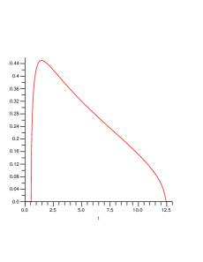
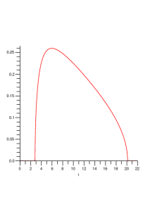
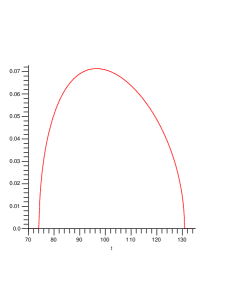
Figure 8. The densities of the measures $\mu_{\lambda}(dt)$, for $\lambda=2$, $3$, and $10$, from left to right.

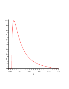
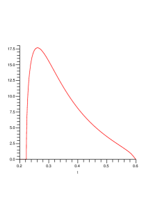
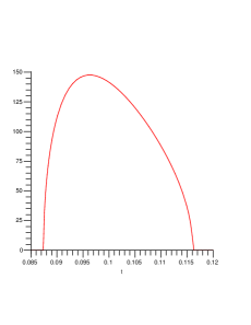
Figure 9. The densities of the spectral measures $(1/\sqrt{\cdot}\,)_{\ast}\mu_{\lambda}(dt)$ of the operators $|\lambda-c|^{-1}$ for $\lambda=2$, $3$, and $10$, from left to right. Note that $|R_{c}(\lambda)|^{2}=[(\lambda-c^{\ast})(\lambda-c)]^{-1}$ has the same distribution as $[(\lambda-c)(\lambda-c^{\ast})]^{-1}=|\lambda-c|^{-2}$ since the von Neumann algebra generated by $c$ is tracial; hence the density of $|\lambda-c|^{-1}$ is the same as the density of $|R_{c}(\lambda)|$.

3. Resolvents in the General $\mathscr{R}$-Diagonal Case

This section is largely devoted to the proof of Theorem 1.1. The direct calculations used in Section 2 are not available in this case: for a general $\mathscr{R}$-diagonal operator $a$, it is far more difficult to find a closed-formula for the $\mathscr{R}$-transform of $|\lambda-a|^{2}$. Nevertheless, in Section 2.2, we determined the support of the measure through critical points, following [5]; through a similar approach, we will be able to calculate the norm of $R_{a}(\lambda)$ to leading order as it tends to $\infty$, for any $\mathscr{R}$-diagonal operator $a$.

Let $a$ be $\mathscr{R}$-diagonal in a $\mathrm{II}_{1}$-factor $\mathscr{A}$. Expanding $\mathscr{A}$ if necessary, we may choose a Haar unitary $u$ $\ast$-free from $a$. It is easy to check that $au$ has the same $\ast$-distribution as $a$; indeed, this can be used as a definition for $\mathscr{R}$-diagonality (cf. [15]). As such, for $\lambda>0$,

$$|a-\lambda|^{2}\mathop{\sim}_{\ast\mathcal{D}}|au-\lambda|^{2}=(au-\lambda)(u^{\ast}a^{\ast}-\lambda)=(a-\lambda u^{\ast})uu^{\ast}(a^{\ast}-\lambda u)=|a-\lambda u^{\ast}|^{2}.$$ (3.1)

Hence, the spectral measure of $|a-\lambda|$ is the same as that of $|a-\lambda u^{\ast}|$, and $(a,\lambda u^{\ast})$ are $\ast$-free $\mathscr{R}$-diagonal elements. We may now employ the following tool for calculating the $\mathscr{R}$-transform of a sum.

Proposition 3.1.

Let $a,b$ be $\ast$-free $\mathscr{R}$-diagonal elements, and for any self-adjoint element $x$ let $\mu_{x}$ denote its spectral measure. For any Borel probability measure $\mu$ on $\mathbb{R}$, denote by $\tilde{\mu}$ the symmetrization of $\mu$: for any Borel set $B\subseteq\mathbb{R}$, $\tilde{\mu}(B)=\frac{1}{2}(\mu(B)+\mu(-B))$. Then

$$\tilde{\mu}_{|a+b|}=\tilde{\mu}_{|a|}\boxplus\tilde{\mu}_{|b|}.$$ (3.2)

Proof.

This is proved in Proposition 5.2 in [14]. A different proof is given in Proposition 3.5 in [4]. ∎

Applying Equation 3.2 to the preceding discussion, we have

$$\tilde{\mu}_{|a-\lambda|}=\tilde{\mu}_{|a-\lambda u^{\ast}|}=\tilde{\mu}_{|a|}\boxplus\tilde{\mu}_{|\lambda u^{\ast}|}.$$

Of course, $|\lambda u^{\ast}|=\lambda$ for $\lambda>0$, and so $\tilde{\mu}_{|\lambda u^{\ast}|}=\frac{1}{2}(\delta_{\lambda}+\delta_{-\lambda})$. Therefore, the associated Cauchy transform is $\frac{1}{2}(\frac{1}{z-\lambda}+\frac{1}{z+\lambda})=\frac{z}{z^{2}-\lambda^{2}}$. Solving the equation $w=\frac{z}{z^{2}-\lambda^{2}}$ for $z$ yields $z=\frac{1\pm\sqrt{1+4\lambda^{2}w^{2}}}{2w}$, and so Equation 1.3 yields that

$$\mathscr{R}_{\tilde{\mu}_{|\lambda u^{\ast}|}}(w)=\frac{1+\sqrt{1+4\lambda^{2}w^{2}}}{2w}-\frac{1}{w}=\frac{\sqrt{1+4\lambda^{2}w^{2}}-1}{2w}$$

(the sign of the square root is chosen so that $\mathscr{R}$ maps $\mathbb{C}_{+}$ into itself). Employing, finally, the additivity of the $\mathscr{R}$-transform over free convolution, we have the following.

Proposition 3.2.

Let $a$ be $\mathscr{R}$-diagonal. Denote by $\mu$ the symmetrization $\tilde{\mu}_{|a|}$, and let $\mu_{\lambda}$ denote the symmetrization $\tilde{\mu}_{|a-\lambda|}$. Then

$$\mathscr{R}_{\mu_{\lambda}}(z)=\mathscr{R}_{\mu}(z)+\frac{\sqrt{1+4\lambda^{2}z^{2}}-1}{2z},\quad\text{for small }z\in\mathbb{C}_{+}.$$ (3.3)

Remark 3.3.

If a measure $\mu$ is supported in $[0,\infty)$, then $\mu$ and $\tilde{\mu}$ contain the same information. Hence, Proposition 3.2 actually allows the determination of the spectral measure of $|\lambda-a|$. Despite this, a direct derivation of $G_{\mu}$ from $G_{\tilde{\mu}}$ is not obvious in general (the latter is the odd part of the former). However, both have the same square. That is, if $\square$ is the map $\square(x)=x^{2}$ for $x\in\mathbb{R}$, then the push-forwards $\square_{\ast}\mu=\square_{\ast}\tilde{\mu}$ are equal and so too are the Cauchy transforms in the case that $\mu$ is supported in $[0,\infty)$.

3.1. The $\mathscr{R}$-transform of $|\lambda-c|^{2}$ – analytic approach

To demonstrate the power of Equation 3.3, we will now use it to give an alternate, entirely analytic proof of Theorem 2.2.

Analytic proof of Theorem 2.2.

Let $\nu_{\lambda}$ denote the spectral measure of $|\lambda-c|^{2}=(\lambda-c)(\lambda-c^{\ast})$, and $\nu=\nu_{0}$ the spectral measure of $|c|^{2}=cc^{\ast}$. Following the notation in Proposition 3.2 and Remark 3.3, with $\mu_{\lambda}=\tilde{\mu}_{|\lambda-c|}$ and $\mu=\tilde{\mu}_{|c|}$, we have $\nu_{\lambda}=\square_{\ast}\mu_{\lambda}$ and $\nu=\square_{\ast}\mu$ where $\square(x)=x^{2}$ for $x\in\mathbb{R}$. Note that $\mu_{|c|}$ is the quarter-circular law $\mu_{|c|}(dt)=\frac{2}{\pi}\sqrt{4-t^{2}}\mathbbm{1}_{[0,2]}(t)\,dt$, and so $\mu$ is the standard semicircle law $\mu(dt)=\frac{1}{\pi}\sqrt{4-t^{2}}\mathbbm{1}_{[-2,2]}(t)\,dt$. Thence $\mathscr{R}_{\mu}(z)=z$, and Equation 3.3 reads

$$\mathscr{R}_{\mu_{\lambda}}(z)=z+\frac{\sqrt{1+4\lambda^{2}z^{2}}-1}{2z},$$ (3.4)

for small $z\in\mathbb{C}_{+}$. In this case, the precise domain is easy to determine since $\mathscr{R}_{\mu}$ is analytic everywhere; the domain of analyticity above is $|z|<\frac{1}{2\lambda}$. Adding $1/z$, Equation 1.3 shows that the functional inverse $G_{\mu_{\lambda}}^{\langle-1\rangle}$ is given by

$$G_{\mu_{\lambda}}^{\langle-1\rangle}(z)=z+\frac{\sqrt{1+4\lambda^{2}z^{2}}+1}{2z},\quad 0<|z|<\frac{1}{2\lambda}.$$

Put $s=\frac{\sqrt{1+4\lambda^{2}z^{2}}+1}{2z}$; then small $|z|$ corresponds to large $|s|$. The quantity $s$ is best characterized as a solution to the quadratic equation $zs^{2}-s-z\lambda^{2}=0$, and so in terms of $s$ we have

$$z=\frac{s}{s^{2}-\lambda^{2}},$$

which evidently makes sense for large $|s|$. Thus, Equation 3.4 may be written in the form

$$\frac{s}{s^{2}-\lambda^{2}}=G_{\mu_{\lambda}}\left(\frac{s}{s^{2}-\lambda^{2}}+s\right),\quad\text{for }|s|\text{ large}.$$ (3.5)

Now, let us consider $G_{\nu_{\lambda}}=G_{\square_{\ast}\mu_{\lambda}}$. We have

$$G_{\nu_{\lambda}}(w^{2})=\int_{\mathbb{R}}\frac{1}{w^{2}-t}\,\square_{\ast}\mu_{\lambda}(dt) =\int_{\mathbb{R}}\frac{1}{w^{2}-t^{2}}\,\mu_{\lambda}(dt)$$ (3.6)

$$=\frac{1}{2w}\int_{\mathbb{R}}\left(\frac{1}{w-t}+\frac{1}{w+t}\right)\,\mu_{\lambda}(dt).$$

A change of variables and the fact that $\mu_{\lambda}$ is symmetric shows that both integrands above have the same integral, and so Equation 3.6 becomes

$$G_{\nu_{\lambda}}(w^{2})=\frac{1}{w}\int_{\mathbb{R}}\frac{1}{w-t}\,\mu_{\lambda}(dt)=\frac{1}{w}G_{\mu_{\lambda}}(w).$$ (3.7)

Substitute $w=\frac{s}{s^{2}-\lambda^{2}}+s$ into Equation 3.5, and Equation 3.7 yields that for large $|s|$,

$$G_{\nu_{\lambda}}\left(\left(\frac{s}{s^{2}-\lambda^{2}}+s\right)^{2}\right)=\left(\frac{s}{s^{2}-\lambda^{2}}+s\right)^{-1}\cdot\frac{s}{s^{2}-\lambda^{2}}=\frac{1}{1+s^{2}-\lambda^{2}}.$$ (3.8)

Inverting $G_{\nu_{\lambda}}$ in Equation 3.8 and again using Equation 1.3, we get for large $|s|$,

$$\mathscr{R}_{\nu_{\lambda}}\left(\frac{1}{1+s^{2}-\lambda^{2}}\right) =G_{\nu_{\lambda}}^{\langle-1\rangle}\left(\frac{1}{1+s^{2}-\lambda^{2}}\right)-(1+s^{2}-\lambda^{2})$$ (3.9)

$$=\left(\frac{s}{s^{2}-a^{2}}+s\right)^{2}-(1+s^{2}-\lambda^{2})$$

$$=\frac{s^{2}(1+s^{2}-\lambda^{2})^{2}}{(s^{2}-\lambda^{2})^{2}}-(1+s^{2}-\lambda^{2}).$$

Finally, set $z=(1+s^{2}-\lambda^{2})^{-1}$, so that large $|s|$ corresponds to small $|z|$. Then

$$1-z=\frac{s^{2}-\lambda^{2}}{s^{2}-\lambda^{2}+1},\quad s^{2}=\frac{1}{w}+\lambda^{2}-1.$$

Substituting into Equation 3.9, we find that for small $z\neq 0$,

$$\mathscr{R}_{\nu_{\lambda}}(z) =(z^{-1}+\lambda^{2}-1)\cdot\frac{1}{(1-z)^{2}}-\frac{1}{z}$$ (3.10)

$$=\frac{z^{-1}-1}{(1-z)^{2}}+\frac{\lambda^{2}}{(1-z)^{2}}-\frac{1}{z}$$

$$=\frac{1}{z(1-z)}-\frac{1}{z}+\frac{\lambda^{2}}{(1-z)^{2}}=\frac{1}{1-z}+\frac{\lambda^{2}}{(1-z)^{2}},$$

which is the desired result. ∎

Remark 3.4.

The above proof is rather shorter than the one in Section 2.1. It relies on the somewhat sophisticated analytic result of Proposition 3.2; on the other hand, the proof in Section 2.1 relies on the sophisticated combinatorial result of Theorem 1.2. The benefit of the combinatorial proof is that it provides a direct explanation for all of the terms in the the $\mathscr{R}$-transform of $\nu_{\lambda}$, which is the reason we’ve included it.

3.2. Analytic Continuation and Roots of $G_{\mu_{\lambda}}$

Our goal is to use Equation 3.2 to determine (to leading order) the smallest positive singular value of $G_{\mu_{\lambda}}$, which is the reciprocal of the spectral radius of the resolvent $R_{a}(\lambda)=(a-\lambda)^{-1}$ of our $\mathscr{R}$-diagonal operator $a$ in the $\mathrm{II}_{1}$–factor $\mathscr{A}$. Let $\varphi$ denote the trace on $\mathscr{A}$. Adding $1/z$ to both sides, rewrite Equation 3.2 in the form

$$G_{\mu_{\lambda}}\left(\mathscr{R}_{\mu}(z)+\frac{1+\sqrt{1+4\lambda^{2}z^{2}}}{2z}\right)=z,\quad\text{for small }z\neq 0.$$ (3.11)

Following Section 4 of [5], we introduce the auxiliary functions

$$h(s) =s\,\varphi\left((aa^{\ast}+s^{2})^{-1}\right),\qquad\qquad\qquad s>0$$ (3.12)

$$h_{\lambda}(s) =s\,\varphi\left(((a-\lambda)(a-\lambda)^{\ast}+s^{2})^{-1}\right),\;\;\lambda,s>0.$$

Then, as proved in Lemma 4.2 in [5],

$$G_{\mu}(is) =-ih(s),\quad\;\;\;s>0$$ (3.13)

$$G_{\mu_{\lambda}}(is) =-ih_{\lambda}(s),\quad\lambda,s>0.$$ (3.14)

Using Equation 3.13 together with the definition of $\mathscr{R}_{\mu}$ in terms of $G_{\mu}$, it follows that there is some large $s_{0}>0$ so that

$$\mathscr{R}_{\mu}(-ih(s))-\frac{1}{ih(s)}=is,\quad s>s_{0}.$$ (3.15)

Combining Equations 3.11 (with $z=-ih(s)$), 3.14, and 3.15, we have

$$h_{\lambda}\left(s-\frac{1}{2h(s)}+\frac{\sqrt{1-4\lambda^{2}h(s)^{2}}}{2h(s)}\right)=h(s),$$ (3.16)

for large $s$ — say $s>s_{\lambda}$ for some $s_{\lambda}>s_{0}$.

Based on Equation 3.16, it was proved in Proposition 4.13 of [5] (see also Lemma 4.8 and Definition 4.9) that $h_{\lambda}(t)$ can be obtained from $h$ for all $t>0$ in the following way.

Proposition 3.5.

For every $t>0$, the equation

$$(s-t)\left(\frac{1}{h(s)-s+t}\right)=\lambda^{2}$$ (3.17)

has a unique solution $s=s(\lambda,t)$ in the interval $(t,\infty)$, and

$$h_{\lambda}(t)=h(s(\lambda,t)),\quad t>0.$$ (3.18)

Corollary 3.6.

Let $s>0$, and assume that $1-4\lambda^{2}h(s)^{2}\geq 0$ and

$$s-\frac{1}{2h(s)}-\frac{\sqrt{1-4\lambda^{2}h(s)^{2}}}{2h(s)}>0.$$

Then

$$h_{\lambda}\left(s-\frac{1}{2h(s)}-\frac{\sqrt{1-4\lambda^{2}h(s)^{2}}}{2h(s)}\right)=h(s).$$ (3.19)

Proof.

Put $t=s-\frac{1}{2s(h)}-\frac{\sqrt{1-4\lambda^{2}h(s)^{2}}}{2h(s)}$. Then $s>t$ (since $h(s)>0$ from Equation 3.12). It is a simple matter to check that $s$ is a solution to Equation 3.17, and therefore $s=s(\lambda,t)$. Hence, Equation 3.19 follows from Equation 3.18. ∎

Remark 3.7.

Comparing Equations 3.16 and 3.19, we see that that point of Corollary 3.6 is that the negative root may also be chosen in the determining equation for $h_{\lambda}$. This results in the similar alternate version of Equation 3.11 in Proposition 3.8 below, identifying what turns out to be the correct singular value of $G_{\mu_{\lambda}}$.

In the following, we assume that $\lambda>\|a\|_{2}$. Since $\mathrm{spec}(a)\subseteq B(0,\|a\|_{2})$ (cf. [4]), $a-\lambda$ is invertible and therefore $\mathrm{supp}\,(\mu_{\lambda})\subseteq\mathbb{R}\setminus(-\delta_{\lambda},\delta_{\lambda})$ for some $\delta_{\lambda}>0$. Therefore $G_{\mu_{\lambda}}$ is defined and analytic in a complex neighbourhood of $0$.

Proposition 3.8.

For all $z$ in a small complex neighbourhood of $0$,

$$G_{\mu_{\lambda}}\left(\mathscr{R}_{\mu}(z)+\frac{1-\sqrt{1+4\lambda^{2}z^{2}}}{2z}\right)=z.$$ (3.20)

Proof.

Since $\mu$ is symmetric, its odd moments are all $0$. Also, since $\square_{\ast}\mu=\mu_{|a|^{2}}$, the even moments are given by

$$m_{2k}(\mu)=\|a\|_{2k}^{2k},\quad k=1,2,\ldots$$

Therefore,

$$G_{\mu}(z)=\frac{1}{z}+\frac{\|a\|_{2}^{2}}{z^{3}}+O\left(\frac{1}{z^{5}}\right),\quad|z|\to\infty.$$

Hence,

$$h(s)=-iG_{\mu}(is)=\frac{1}{s}+\frac{\|a\|_{2}^{2}}{s^{3}}+O\left(\frac{1}{s^{5}}\right),\quad s\to\infty.$$

It follows that

$$\frac{1}{h(s)}=s\left(1-\frac{\|a\|_{2}^{2}}{s^{2}}+O\left(\frac{1}{s^{4}}\right)\right),\quad s\to\infty$$

and

$$\sqrt{1-4\lambda^{2}h(s)^{2}}=1-\frac{2\lambda^{2}}{s^{2}}+O\left(\frac{1}{s^{4}}\right).$$

Taking $t=t(s)$ as in the proof of Corollary 3.6, we have

$$t(s) =s-\frac{1}{2h(s)}-\frac{\sqrt{1-4\lambda^{2}h(s)^{2}}}{2h(s)}$$

$$=(\lambda^{2}-\|a\|_{2}^{2})\frac{1}{s}+O\left(\frac{1}{s^{3}}\right),$$

and therefore $t(s)>0$ for $s>s_{\lambda}^{\prime}$ for some $s_{\lambda}^{\prime}>0$. Thus, by Corollary 3.6,

$$h_{\lambda}(t(s))=h(s)\quad\text{for }s>s_{\lambda}^{\prime}$$

which is precisely the statement of Equation 3.20 in the case $z=-ih(s)$. Since

$$\lim_{z\to 0}\left[\mathscr{R}_{\mu}(z)+\frac{1-\sqrt{1+4\lambda^{2}z^{2}}}{2z}\right]=0,$$

the left-hand-side of Equation 3.20 is well-defined and analytic in a complex neighbourhood of $0$. Hence, as we have shown that the equation holds for all $z$ in an imaginary line segment accumulating at $0$, Equation 3.20 holds everywhere in a complex neighbourhood of $0$. ∎

3.3. Negative Moments

From now on, let us normalize $a$ so that $\|a\|_{2}=1$; we therefore only consider $\lambda>1$. We also assume that $a$ is not Haar unitary, which (under this normalization) is equivalent to the requirement that $\|a\|_{4}>1$. Put

$$M_{\lambda}=\|a-\lambda\|,\quad m_{\lambda}=\|(a-\lambda)^{-1}\|^{-1}.$$

Then

$$\mathrm{supp}\,(\mu_{\lambda})\subseteq[-M_{\lambda},-m_{\lambda}]\cup[m_{\lambda},M_{\lambda}].$$

Moreoever, $\pm m_{\lambda}$ and $\pm M_{\lambda}$ are singular points for the Cauchy transform

$$G_{\mu_{\lambda}}(z)=\int_{\mathbb{R}}\frac{1}{z-x}\mu_{\lambda}(dx),\quad z\in\mathbb{C}-\left([-M_{\lambda},-m_{\lambda}]\cup[m_{\lambda},M_{\lambda}]\right).$$

Our goal is to determine the asymptotic behaviour of $m_{\lambda}$ as $\lambda\downarrow 1$; we will accomplish this through Equation 3.20.

The free cumulants $\kappa_{n}(\mu)$ vanish for odd $n$ since $\mu$ is symmetric, and so $\mathscr{R}_{\mu}$ is given by the power series

$$\mathscr{R}_{\mu}(z)=\kappa_{2}(\mu)z+\kappa_{4}(\mu)z^{3}+\kappa_{6}(\mu)z^{5}+\cdots$$

for $z$ in a complex neighbourhood of $0$. Moreover, since $\mu$ is centred,

$$\kappa_{2}(\mu)=m_{2}(\mu)=\|a\|_{2}^{2}=1$$

and

$$\kappa_{4}(\mu)=m_{4}(\mu)-2=\|a\|_{4}^{4}-2.$$

Define

$$v(a)=\|a\|_{4}^{4}-(\|a\|_{2}^{2})^{2}=\kappa_{4}(\mu)+1.$$ (3.21)

Then $v(a)$ is strictly positive. We have

$$\mathscr{R}_{\mu}(z)=z+(v(a)-1)z^{3}+\kappa_{6}(\mu)z^{5}+O(z^{7}).$$

Now, we may expand $\sqrt{1+4\lambda^{2}z^{2}}$ as a Taylor series about $0$. The result is

$$\frac{1-\sqrt{1+4\lambda^{2}z^{2}}}{2z} =\frac{1}{2z}\left(1-\sum_{\ell=0}^{\infty}\binom{1/2}{\ell}(4\lambda^{2}z^{2})^{\ell}\right)$$

$$=-\sum_{\ell=1}^{\infty}\binom{1/2}{\ell}\lambda^{2\ell}(2z)^{2\ell-1}$$

$$=\sum_{\ell=1}^{\infty}(-1)^{\ell}C_{\ell-1}\lambda^{2\ell}(2z)^{2\ell-1}$$

$$=-\lambda^{2}z+\lambda^{4}z^{3}-2\lambda^{6}z^{5}+\cdots$$

Here $C_{k}$ is the Catalan number $C_{k}=\frac{1}{k+1}\binom{2k}{k}$. Now, following Equation 3.20, define

$$B_{\lambda}(z)=\mathscr{R}_{\mu}(z)+\frac{1-\sqrt{1+4\lambda^{2}z^{2}}}{2z}.$$ (3.22)

From the preceding discussion, $B_{\lambda}$ has a the power series expansion

$$B_{\lambda}(z)=\left(1-\lambda^{2}\right)z+\left(v(a)-1+\lambda^{4}\right)z^{3}+\left(\kappa_{6}(\mu)-2\lambda^{6}\right)z^{5}+O(z^{7}),$$ (3.23)

in a complex neighbourhood of $0$.

By Proposition 3.8, $B_{\lambda}(z)$ and $G_{\mu_{\lambda}}(w)$ are inverse functions of each other when both $|z|$ and $|w|$ are small. Since $\mathrm{supp}\,(\mu_{\lambda})\subseteq\mathbb{R}\setminus(-\delta_{\lambda},\delta_{\lambda})$ with $\delta_{\lambda}>0$, we have for $|w|<\delta_{\lambda}$,

$$G_{\mu_{\lambda}}(w) =\int_{\mathbb{R}\setminus(-\delta_{\lambda},\delta_{\lambda})}\frac{1}{w-x}\mu_{\lambda}(dx)$$ (3.24)

$$=-\int_{\mathbb{R}\setminus(-\delta_{\lambda},\delta_{\lambda})}\frac{1}{x}\left(1+\frac{w}{x}+\frac{w^{2}}{x^{2}}+\cdots\right)\,\mu_{\lambda}(dx)$$

$$=-\left(m_{-2}(\mu_{\lambda})\,w+m_{-3}(\mu_{\lambda})\,w^{2}+m_{-4}(\mu_{\lambda})\,w^{3}+\cdots\right),$$

where

$$m_{-k}(\mu_{\lambda})=\int_{\mathbb{R}}x^{-k}\mu_{\lambda}(dx),\quad k=1,2,\ldots$$ (3.25)

are the negative moments of $\mu_{\lambda}$. Again, since $\mu_{\lambda}$ is symmetric, $m_{-k}(\mu_{\lambda})=0$ for $k$ odd. We will now use the Lagrange inversion formula, together with Equations 3.23 and 3.24, to express the even negative moment $m_{-2\ell}(\mu_{\lambda})$ in terms of the free cumulants $\kappa_{2}(\mu_{\lambda}),\kappa_{4}(\mu_{\lambda}),\ldots,\kappa_{2\ell}(\mu_{\lambda})$ for $\ell\in\mathbb{N}$. In particular, as can be easily calculated directly,

$$m_{-2}(\mu_{\lambda})=\frac{1}{\lambda^{2}-1},\quad m_{-4}(\mu_{\lambda})=\frac{\lambda^{4}-1+v(a)}{(\lambda^{2}-1)^{4}}.$$ (3.26)

Lemma 3.9.

Let $v>0$. The inverse of the function

$$F(z)=z-vz^{3}$$

has the power series expansion

$$F^{\langle-1\rangle}(w)=\sum_{k=0}^{\infty}C^{(2)}_{k}v^{k}\,w^{2k+1},$$

where $C^{(2)}_{k}=\frac{1}{2k+1}\binom{3k}{k}$.

Remark 3.10.

The numbers $C^{(2)}_{k}$ in Lemma 3.9 are the $p=2$ case of the Fuss-Catalan numbers

$$C^{(p)}_{k}=\frac{1}{pk+1}\binom{(p+1)k}{k}.$$

Note that when $p=1$ we recover the standard Catalan numbers. The appearance of these combinatorially interesting numbers in free probability theory is discussed at length in [10] and [12], in addition to more recent papers and preprints [1], [8], and [9].

Proof.

Since $F$ is odd, so is its inverse. Write the (yet-to-be-determined) coefficients of $F^{\langle-1\rangle}$ as $F^{\langle-1\rangle}(w)=w+b_{3}w^{3}+b_{5}w^{5}+\cdots$. Since $F$ is analytic at $0$ and $F^{\prime}(0)\neq 0$, the Lagrange inversion formula states that

$$b_{2k+1}=\frac{1}{2k+1}\mathrm{Res}\left(F(z)^{-(2k+1)},0\right).$$

Writing $F(z)^{-(2k+1)}=(1-vz^{2})^{-(2k+1)}\,\cdot z^{-2k}\frac{1}{z}$, we see that the residue in question is the coefficient of $z^{2k}$ in the power series expansion of $(1-vz^{2})^{-(2k+1)}$, which is equal to

$$v^{k}\frac{(2k+1)(2k+2)\cdots(3k)}{k!}=v^{k}\binom{3k}{k}.$$

This proves the lemma. ∎

Theorem 3.11.

Let $k$ be a non-negative integer. Then as $\lambda\downarrow 1$,

$$m_{-2k-2}(\mu_{\lambda})\sim C^{(2)}_{k}\frac{v(a)^{k}}{(\lambda^{2}-1)^{3k+1}}.$$ (3.27)

Remark 3.12.

The appearance of the Fuss-Catalan numbers to leading order in Equation 3.27 for the negative moments of $\mu_{\lambda}$ begs for a combinatorial explanation. Indeed, there is a completely combinatorial proof of Theorem 3.11; this is the content of Section 4.1. What’s more, the lower bound of Theorem 1.1 can be proved with a simple estimate directly from Theorem 3.11; this is the content of Section 4.2.

Proof.

Put $v=v(a)>0$. Referring to Equation 3.22, rescale $B_{\lambda}$ and set

$$F_{\lambda}(z)=-(\lambda^{2}-1)^{-3/2}B_{\lambda}\left((\lambda^{2}-1)^{1/2}z\right).$$ (3.28)

Then following Equation 3.23 and using Equation 3.26, we have

$$F_{\lambda}(z)=z-(v-1+\lambda^{4})z^{3}-(\lambda^{2}-1)(\kappa_{6}(\mu)-2\lambda^{6})z^{5}-(\lambda^{2}-1)^{2}(\kappa_{8}+5\lambda^{6})z^{7}+\cdots$$

Hence, the coefficients in the power series for $F_{\lambda}(z)$ converge to the coefficients in the power series

$$F(z)=z-vz^{3}+0z^{5}+0z^{7}=z-vz^{3}$$

as in Lemma 3.9. Therefore, by the continuity of the Lagrange inversion formula, the coefficient $b_{2k+1}^{(\lambda)}$ of $z^{2k+1}$ in $F_{\lambda}^{\langle-1\rangle}(z)$ converges by Lemma 3.9 to $C^{(2)}_{k}v^{k}$ as $\lambda\downarrow 1$; that is,

$$\lim_{\lambda\downarrow 1}b^{(\lambda)}_{2k+1}=C^{(2)}_{k}v^{k}.$$ (3.29)

Now inverting Equation 3.28 (setting $u=(\lambda^{2}-1)z$),

$$B_{\lambda}(u)=-(\lambda^{2}-1)^{3/2}F_{\lambda}\left(\frac{u}{(\lambda^{2}-1)^{1/2}}\right),$$

and therefore for $|w|$ small,

$$G_{\mu_{\lambda}}(w)=B_{\lambda}^{\langle-1\rangle}(w) =(\lambda^{2}-1)^{1/2}\;F_{\lambda}^{\langle-1\rangle}\left(-\frac{w}{(\lambda^{2}-1)^{3/2}}\right)$$ (3.30)

$$=-(\lambda^{2}-1)^{1/2}\;F_{\lambda}^{\langle-1\rangle}\left(\frac{w}{(\lambda^{2}-1)^{3/2}}\right),$$

the last equality following from the fact that $F_{\lambda}^{\langle-1\rangle}$ is an odd function.

Now, $m_{-2k-2}(\mu_{\lambda})$ is the coefficient of $w^{2k+1}$ in the power series expansion of $G_{\mu_{\lambda}}(w)$, and so by Equations 3.30,

$$m_{-2k-2}(\mu_{\lambda})=(\lambda^{2}-1)^{1/2}(\lambda^{2}-1)^{-3/2}b^{(\lambda)}_{2k+1}\left((\lambda^{2}-1)^{-3/2}\right)^{2k+1}=(\lambda^{2}-1)^{-(3k+1)}b^{(\lambda)}_{2k+1},$$

and hence the Theorem follows from Equation 3.29. ∎

3.4. Proof of Theorem 1.1

The convergence of the coefficients of $F_{\lambda}$ to those of $F$ as $\lambda\downarrow 1$ is not enough to prove our main theorem. In fact, the convergence is stronger, as we now show. Choose $\varrho\in(0,\frac{1}{4})$ small enough that $\mathscr{R}_{\mu}$ is analytic in $B(0,\varrho)$. Then

$$B_{\lambda}(z)=\mathscr{R}_{\mu}(z)+\frac{1-\sqrt{1+4\lambda^{2}z^{2}}}{2z}$$

is analytic in $B(0,\varrho)$ for all $\lambda\in(1,2)$. Thence, with $F_{\lambda}$ as in Equation 3.28, $F_{\lambda}$ is analytic and well-defined in $B(0,\varrho/\sqrt{\lambda^{2}-1})$. Note that $\varrho/\sqrt{\lambda^{2}-1}\to\infty$ as $\lambda\downarrow 1$.

Proposition 3.13.

With $F_{\lambda}$ as in Equation 3.28 and $F$ as in Lemma 3.9, $F_{\lambda}(z)\to F(z)$ uniformly on compact subsets of $\mathbb{C}$ as $\lambda\downarrow 1$.

Proof.

We claim there exists a constant $C>0$ and a $\varrho^{\prime}>0$ such that, for all $z\in B(0,\varrho^{\prime})$ and all $\lambda\in(1,2)$,

$$|B_{\lambda}(z)-(1-\lambda^{2})z-(v(a)-1+\lambda^{4})z^{3}|\leq C|z|^{5}.$$ (3.31)

For the moment, assume Equation 3.31 has been proved. Then setting $w=(\lambda^{2}-1)^{1/2}z$,

$$|F_{\lambda}(z)-z +(v(a)-1+\lambda^{4})z^{3}|$$

$$= |-(\lambda^{2}-1)^{-3/2}B_{\lambda}\left((\lambda^{2}-1)^{1/2}z\right)-z+(v(a)-1+\lambda^{4})z^{3}|$$

$$= \left|-(\lambda^{2}-1)^{-3/2}B_{\lambda}(w)-\frac{w}{(\lambda^{2}-1)^{1/2}}+(v(a)-1+\lambda^{4})\left(\frac{w}{(\lambda^{2}-1)^{1/2}}\right)^{3}\right|$$

$$= (\lambda^{2}-1)^{-3/2}|B_{\lambda}(w)-(1-\lambda^{2})w-(v(a)-1+\lambda^{4})w^{3}|,$$

and by Equation 3.31 this is

$$\leq(\lambda^{2}-1)^{-3/2}\,C|w|^{5}=(\lambda^{2}-1)^{-3/2}\,C|(\lambda^{2}-1)^{1/2}z|^{5}=C(\lambda^{2}-1)|z|^{5}$$

for $z\in B(0,\varrho^{\prime}/\sqrt{\lambda^{2}-1})$. Thus, we have

$$F_{\lambda}(z)-F(z)=F_{\lambda}(z)-(z-v(a)z^{3})=F_{\lambda}(z)-z+v(a)z^{3}=F_{\lambda}(z)-z+(v(a)-1+\lambda^{4})z^{3}+(1-\lambda^{4})z^{3},$$

and so

$$|F_{\lambda}(z)-F(z)| \leq|F_{\lambda}(z)-z+(v(a)-1+\lambda^{4})z^{4}|+(\lambda^{4}-1)|z|^{3}$$

$$\leq(\lambda^{4}-1)|z|^{3}+C(\lambda^{2}-1)|z|^{5}.$$

This proves the proposition. Hence, it remains only to verify the estimate of Equation 3.31. Referring to Equation 3.23,

$$B_{\lambda}(z)-(1-\lambda^{2})z-(v(a)-1+\lambda^{4})z^{3}=\sum_{\ell=3}^{\infty}[\kappa_{2\ell}(\mu)-(-1)^{\ell}C_{\ell-1}\lambda^{2\ell}]\,z^{2\ell-1}.$$

It is convenient to break this up as a sum of two power series, $B_{\lambda}(z)=D(z)+C_{\lambda}(z)$ where

$$D(z) =\kappa_{6}(\mu)z^{5}+\kappa_{8}(\mu)z^{7}+\cdots$$

$$C_{\lambda}(z) =-C_{2}\lambda^{6}z^{5}+C_{3}\lambda^{8}z^{7}-\cdots$$

Now, $D(z)$ is a truncation of the power series for $\mathscr{R}_{\mu}(z)$, which is convergent and analytic in $B(0,\varrho)$; as $D(z)$ has a $0$ of order $5$ as $0$, it follows that there is a constant $C_{1}\geq|\kappa_{6}(\mu)|$ such that $|D(z)|\leq c_{1}|z|^{5}$ in that neighbourhood of $0$. On the other hand, note that $C_{k}<4^{k}$, and so with $\lambda<2$,

$$|C_{\lambda}(z)|\leq 2^{10}|z|^{5}+2^{14}|z|^{7}+\cdots=2^{10}\frac{|z|^{5}}{1-16|z|^{2}},$$

and so choosing $\varrho^{\prime}<1/4$, we may choose a constant $c_{2}>0$ with $|C_{\lambda}(z)|\leq c_{2}|z|^{5}$ for $z\in B(0,\varrho^{\prime})$. Setting $C=c_{1}+c_{2}$, this proves Equation 3.31. ∎

Lemma 3.14.

For all $\lambda>1$ sufficiently close to $1$, there is a unique $x_{\lambda}\in(0,\frac{1}{\sqrt{v}})$ (where $v=v(a)$) such that the real analytic function $x\mapsto F_{\lambda}^{\prime}(x)$ has the following sign variation in $[-\frac{1}{\sqrt{v}},\frac{1}{\sqrt{v}}]$.

• $F_{\lambda}^{\prime}(x)>0$ for $x\in(-x_{\lambda},x_{\lambda})$.

• $F_{\lambda}^{\prime}(x)=0$ for $x=\pm x_{\lambda}$.

• $F_{\lambda}^{\prime}(x)<0$ for $x_{r}<|x|\leq\frac{1}{\sqrt{v}}$.

Moreover, $x_{\lambda}\to\frac{1}{\sqrt{3v}}$ and $F_{\lambda}(x_{\lambda})\to\left(\frac{4}{27v}\right)^{1/2}$ as $\lambda\downarrow 1$.

Proof.

The uniform convergence of $F_{\lambda}$ to $F$ on compact subsets of $\mathbb{C}$ implies by standard complex analysis that $F_{\lambda}^{(p)}$ (the $p$th derivative of $F_{\lambda}$) converges uniformly to $F^{(p)}$ on compact subsets of $\mathbb{C}$, for each $p\in\mathbb{N}$. Since $F^{(3)}(x)=-6v<0$, we can choose $\lambda_{0}>1$ such that for all $\lambda\in(1,\lambda_{0})$,

$$F_{\lambda}^{(3)}(x)<0,\quad\text{for}\quad|x|\leq\frac{1}{\sqrt{v}}.$$ (3.32)

Hence, for $\lambda\in(1,\lambda_{0})$, $F_{\lambda}^{\prime\prime}$ is strictly decreasing on $[-\frac{1}{\sqrt{v}},\frac{1}{\sqrt{v}}]$. Moreover, $F_{\lambda}^{\prime\prime}(0)=0$ since $F_{\lambda}$ is an odd function. Therefore,

$$F_{\lambda}^{\prime\prime}(x)<0\quad\text{for }\quad\textstyle{x\in(0,\frac{1}{\sqrt{v}})}.$$

Hence $F_{\lambda}^{\prime}$ is strictly decreasing on $[0,\frac{1}{\sqrt{v}}]$ for $\lambda\in(1,\lambda_{0})$. Moreover,

$$\lim_{\lambda\downarrow 1}F_{\lambda}^{\prime}(0) =F^{\prime}(0)=1$$

$$\lim_{\lambda\downarrow 1}F_{\lambda}^{\prime}(\textstyle{\frac{1}{\sqrt{v}}}) =F^{\prime}(\textstyle{\frac{1}{\sqrt{v}}})=-2.$$

Therefore we can choose $\lambda_{1}\in(0,\lambda_{0}]$ such that

$$F_{\lambda}^{\prime}(0)>0\quad\text{and}\quad F_{\lambda}^{\prime}(\textstyle{\frac{1}{\sqrt{v}}})<0\quad\text{for}\quad 0<\lambda<\lambda_{1}.$$

Hence, for all such $\lambda$, the equation $F_{\lambda}^{\prime}(x)=0$ has exactly one solution $x_{\lambda}$ in the interval $(0,\frac{1}{\sqrt{v}})$, and $F_{\lambda}^{\prime}(x)>0$ for $x\in[0,x_{\lambda})$, while $F_{\lambda}^{\prime}(x)<0$ for $x\in(x_{\lambda},\frac{1}{\sqrt{v}})$. Since $F_{\lambda}^{\prime}$ is an even function, the above-stated sign variation holds for all $\lambda\in(1,\lambda_{1})$.

Now, note that $\frac{1}{\sqrt{3v}}$ is a critical point for $F$, and also for $\epsilon\in(0,\frac{1}{2})$,

$$F^{\prime}(\textstyle{\frac{1-\epsilon}{\sqrt{3v}}})>0\quad\text{and}\quad F^{\prime}(\textstyle{\frac{1+\epsilon}{\sqrt{3v}}})<0.$$

Therefore, by the uniform convergence,

$$F_{\lambda}^{\prime}(\textstyle{\frac{1-\epsilon}{\sqrt{3v}}})>0\quad\text{and}\quad F_{\lambda}^{\prime}(\textstyle{\frac{1+\epsilon}{\sqrt{3v}}})<0,$$

for $\lambda>1$ sufficiently close to $1$. It follows that $\frac{1-\epsilon}{\sqrt{3v}}<x_{\lambda}<\frac{1+\epsilon}{\sqrt{3v}}$ eventually as $\lambda\downarrow 1$. This shows that $\lim_{\lambda\downarrow 1}x_{\lambda}=\frac{1}{\sqrt{3v}}$, and by the uniform convergence of $F_{\lambda}$ to $F$ on $[-v,v]$, it follows that

$$\lim_{\lambda\downarrow 1}F_{\lambda}(x_{\lambda})=F(\textstyle{\frac{1}{\sqrt{3v}}})=\left(\frac{4}{27v}\right)^{1/2},$$

as required. ∎

This finally brings us to the proof of the main theorem.

Proof of Theorem 1.1.

It follows from Lemma 3.14 that for all $\lambda>1$ sufficiently close to $1$, $F_{\lambda}^{\langle-1\rangle}$ has an analytic extension to a complex open neighbourhood of the interval $(-F_{\lambda}(x_{\lambda}),F_{\lambda}(x_{\lambda}))$, but that both endpoints of the interval are singular points of $F_{\lambda}^{\langle-1\rangle}$. Since

$$G_{\mu_{\lambda}}(z)=-(\lambda^{2}-1)^{1/2}F_{\lambda}^{\langle-1\rangle}\left(\frac{z}{(\lambda^{2}-1)^{3/2}}\right)$$

for $|z|$ small, it follows that $G_{\mu_{\lambda}}$ has an analytic extension to a complex neighbourhood of

$$I_{\lambda}=\left(-(\lambda^{2}-1)^{3/2}F_{\lambda}(x_{\lambda}),(\lambda^{2}-1)^{3/2}F_{\lambda}(x_{\lambda})\right),$$

but the endpoints of the interval are singular points for $G_{\mu_{\lambda}}$. Therefore,

$$\pm(\lambda^{2}-1)^{3/2}F_{\lambda}(x_{\lambda})\in\mathrm{supp}\,(\mu_{\lambda}),$$

while

$$I_{\lambda}\cap\mathrm{supp}\,(\mu_{\lambda})=\varnothing.$$

Since $\mu_{\lambda}=\tilde{\mu}_{|a-\lambda|}$, it follows that

$$\|(a-\lambda)^{-1}\|=\frac{1}{(\lambda^{2}-1)^{3/2}F_{\lambda}(x_{\lambda})},$$

for $\lambda>1$ sufficiently close to $1$. As $\lambda\downarrow 1$, this tends (by Lemma 3.14) to

$$\frac{1}{2^{3/2}}\,\frac{1}{(\lambda-1)^{3/2}}\,\left(\frac{27v}{4}\right)^{1/2},$$

thus proving Theorem 1.1. ∎

4. The Combinatorics of Negative Moments

In this final section, we provide a new combinatorial framework for even moments of the absolute resolvent of an $\mathscr{R}$-diagonal operator (that is, negative moments of $|\lambda-a|^{2}$ where $a$ is $\mathscr{R}$-diagonal and $\lambda>\|a\|_{2}$). This approach, through partition structure diagrams, is used in Section 4.1 below to give a new proof of (a more refined statement of) Theorem 3.11. In Section 4.2, we show how knowledge of these moments alone yields the sharp lower bound of Theorem 1.1.

4.1. Partition Structure Diagrams

Let us normalize $a$ once again so that $\|a\|_{2}=1$, and let $\lambda>1$. For convenience, let $r=1/\lambda\in(0,1)$. Then we may rewrite $R_{a}(\lambda)=(\lambda-a)^{-1}=r(1-ra)^{-1}$. Hence, for any positive integer $k$,

$$|R_{a}(\lambda)|^{2(k+1)} =[(\lambda-a)(\lambda-a^{\ast})]^{-(k+1)}=\left[(\lambda-a^{\ast})^{-1}(\lambda-a)^{-1}\right]^{k+1}$$

$$=r^{2(k+1)}\left[(1-ra^{\ast})^{-1}(1-ra)^{-1}\right]^{k+1}.$$

Expanding the geometric series inside this term gives

$$|R_{a}(\lambda)|^{2(k+1)}=r^{2(k+1)}\left[\sum_{n\geq 0}r^{n}a^{\ast n}\,\sum_{m\geq 0}r^{m}a^{m}\right]^{k+1}.$$

Expanding this product of summations we have

$$|R_{a}(\lambda)|^{2(k+1)}=r^{2(k+1)}\sum_{n_{0},\ldots,n_{k}\atop m_{0},\ldots,m_{k}}r^{n_{0}+\cdots+n_{k}+m_{0}+\cdots+m_{k}}a^{\ast n_{0}}a^{m_{0}}\cdots a^{\ast n_{k}}a^{m_{k}}.$$

Since $a$ is $\mathscr{R}$-diagonal, it is rotationally-invariant, and so only monomials with equal numbers of $a$ and $a^{\ast}$ can have non-zero mean in the state $\varphi$. Thus,

$$m_{-2k-2}(\mu_{\lambda})=\varphi\left(|R_{a}(\lambda)|^{2(k+1)}\right)=r^{2(k+1)}\sum_{{n_{0},\ldots,n_{k}\atop m_{0},\ldots,m_{k}}\atop n_{0}+\cdots+n_{k}=m_{0}+\cdots+m_{k}}r^{2(n_{0}+\cdots+n_{k})}\,\varphi(a^{\ast n_{0}}a^{m_{0}}\cdots a^{\ast n_{k}}a^{m_{k}}).$$ (4.1)

We now employ Equation 1.6 expanding the mean as

$$\varphi(a^{\ast n_{0}}a^{m_{0}}\cdots a^{\ast n_{k}}a^{m_{k}})=\sum_{\pi\in NC(n_{0},m_{0},\ldots,n_{k},m_{k})}\kappa_{\pi}[a^{\ast,n_{0}},a^{,m_{0}},\ldots,a^{\ast,n_{k}},a^{,m_{k}}].$$

Notation 4.1.

The following shorthand notations will make the text below far more readable.

• Let $\mathbf{n},\mathbf{m}$ stand for multi-indices $(n_{0},\ldots,n_{k})$ and $(m_{0},\ldots,m_{k})$.

• The sum of a multi-index $n_{0}+\cdots+n_{k}$ is denoted $|\mathbf{n}|$.

• Denote the interleaved multi-index $(n_{0},m_{0},\ldots,n_{k},m_{k})$ as $\mathbf{n}\merge\mathbf{m}$.

• Denote the cumulant $\kappa_{2\ell}[a,a^{\ast},\ldots,a,a^{\ast}]$ as $\alpha_{\ell}(a)$; note, by traciality, $\alpha_{\ell}(a)$ is also equal to the cumulant $\kappa_{2\ell}[a^{\ast},a,\ldots,a^{\ast},a]$.

Because $a$ is $\mathscr{R}$-diagonal, the mixed cumulant $\kappa_{\pi}[a^{\ast,n_{0}},a^{,m_{0}},\ldots,a^{\ast,n_{k}},a^{,m_{k}}]$ is a product of terms $\alpha_{\ell}(a)$ with $\ell$ between $1$ and $k+1$. The precise product is determined by the block profile of the partition $\pi$.

Definition 4.2.

Let $\mathbf{n},\mathbf{m}$ be multi-indices, and let $\pi\in NC(\mathbf{n}\merge\mathbf{m})$. The block profile $\mathbf{pr}(\pi)$ is the multi-index $\mathbf{p}=(p_{1},\ldots,p_{k+1})$, where $p_{1}$ is the number of blocks in $\pi$ of size $2$, $p_{2}$ is the number of blocks in $\pi$ of size $4$, and so forth. Note that, in this case, the sum $|\mathbf{n}|+|\mathbf{m}|=2|\mathbf{n}|$ is equal to $2p_{1}+4p_{2}+\cdots+2(k+1)p_{k+1}$. Denote this number as $\varepsilon(\mathbf{p})$,

$$\varepsilon(\mathbf{p})=2\sum_{j=1}^{k+1}j\,p_{j}.$$

By definition, if $\mathbf{pr}(\pi)=\mathbf{p}$, then the mixed cumulant $\kappa_{\pi}[a^{\ast,n_{0}},a^{,m_{0}},\ldots,a^{\ast,n_{k}},a^{,m_{k}}]$ is equal to $\alpha_{1}(a)^{p_{1}}\cdots\alpha_{k+1}(a)^{p_{k+1}}$. Denote this product as $\alpha(a)^{\mathbf{p}}$. We can thus re-index the sum in Equation 4.1 as follows:

$$m_{-2k-2}(\mu_{\lambda})=r^{2(k+1)}\sum_{\mathbf{n},\mathbf{m}\atop|\mathbf{n}|=|\mathbf{m}|}\sum_{\pi\in NC(\mathbf{n}\merge\mathbf{m})}\alpha(a)^{\mathbf{pr}(\pi)}\,r^{\varepsilon(\mathbf{pr}(\pi))}.$$ (4.2)

The idea now is to reindex the sum over $\mathbf{n},\mathbf{m}$ and $\pi$ in terms of a new set of combinatorial objects: partition structure diagrams. Set $V_{k+1}=\{(1,1),(1,\ast),(2,1),(2,\ast),\ldots,(k+1,1),(k+1,\ast)\}$; view $V_{k+1}$ as vertices (in sequence) on the boundary of a disc. It is possible to encode all the information in a pair $\mathbf{n},\mathbf{m}$ and a partition $\pi\in NC(\mathbf{n}\merge\mathbf{m})$ succinctly in terms of $V_{k+1}$, as follows. Consider subsets of $V_{k+1}$ of the form $P=\{(v_{1},1),(w_{1},\ast),\ldots,(v_{\ell},1),(w_{\ell},\ast)\}$ where $v_{1}\leq w_{1}<v_{2}\leq w_{2}<\cdots<v_{\ell}\leq w_{\ell}$ and $\ell\leq k+1$; viewed on the disc, $P$ is a convex $2\ell$-gon whose vertices alternate between $1$ and $\ast$. (Note: $\ell=1$ is allowed – a $2$-gon is a line-segment.)

For any $\mathbf{n},\mathbf{m},\pi\in NC(\mathbf{n}\merge\mathbf{m})$, assign non-negative integers to the polygonal subset $P$ of $V_{k+1}$ as follows. $P$ is assigned the number of $2\ell$-blocks in $\pi$ that connect vertices in sequence as follows: a vertex from the $v_{1}$ run of $1$s, then a vertex from the $w_{1}$ run of $\ast$s, then a vertex from the $v_{2}$ run of $1$s, and so forth. As such, a triple $\mathbf{n},\mathbf{m},\pi$ yields an labeled polygonal diagram, or LPD. Figure demonstrates this procedure.

Figure 10. A partition in $\pi\in NC(\mathbf{n}\merge\mathbf{m})$, where $\mathbf{n}=(3,4,2,5,1,1)$ and $\mathbf{m}=(4,2,3,2,4,1)$, together with the resulting labeled polygonal diagram. $2$-gons are drawn as straight line-segments, while non-degenerate polygons are drawn non-convex so all lines and labels are clearly visible. Those polygonal subsets not appearing in the LPD have label $0$.

Note, in Figure 10, those polygons with more than $2$ sides have label $1$ or $0$. This is a general phenomenon, as the reader can easily check: since $\pi$ is non-crossing, there can be at most one block of size $2\ell$ ($\ell>1$) connecting a set of vertices in the same $1$- and $\ast$-runs. However, this restriction does not apply to $2$-blocks: there can be many nested pairings, as seen in Figure 10. There is a simple geometric explanation here: for fixed $\mathbf{n},\mathbf{m}$, the map from $\pi$ to the LPD (viewed as a collection of inscribed polygons in a disc) is a compression. Two $(2\ell)$-blocks ($\ell>1$) in $\pi$ with the same image under the compression would have non-trivially intersecting interiors, and therefore would cross. Since $2$-blocks have no interior, on the other hand, they can compress to the same $2$-gon without crossing.

Not every LPD is the compression of a partition: as explained, to come from a partition, the label of any non-degenerate polygon must be $0$ or $1$. But there are further restrictions. For example, if the label of the $2$-gon joining $(2,1)$ to $(4,\ast)$ in Figure 10 were non-zero, no non-crossing pairing could compress to that LPD. The restriction, of course, is that the polygons with non-zero label in the LPD should be non-crossing as well. This brings us to the notion of a(n unlabled) partition structure diagram.

Definition 4.3.

A partition structure diagram or PSD with $2(k+1)$ vertices, $D$, is a collection of polygons, each with an even number of sides, inscribed in the disc $V_{k+1}$, with the following additional properties:

• The vertices of any polygon $P\in D$ are among the vertices $V_{k+1}$, and any edge in $P$ connects a $1$ with a $\ast$.

• The intersection of any two polygons in $P$ has $0$ area; that is, if any two intersect, it is along a common set of edges or vertices only.

Denote the set of all such $D$ by $PSD_{k+1}$.

Following our discussion, if $D=(P_{1},\ldots,P_{s})$ is a PSD, and we label it with positive integers $L(P_{1}),\ldots,L(P_{s})$, then it can only be the compression of a partition in some $NC(\mathbf{n},\mathbf{m})$ if the label of any non-degenerate polygon in $D$ is $1$. Call such a labeling $L$ valid.

In fact, it is easy to see that any such labeled PSD is the compression of a unique partition. Here is the algorithm: begin by decompressing each labeled $2$-gon into the requisite number of nested $2$-blocks. Then, to avoid crossings, each remaining non-degenerate polygon can be inserted in one and only one way – closer to the center of the disc than any surrounding $2$-blocks.

Hence, there is a bijection between the set $\{(\mathbf{n},\mathbf{m},\pi)\,;\,\mathbf{n},\mathbf{m}\in\mathbb{N}^{k+1},|\mathbf{n}|=|\mathbf{m}|,\pi\in NC(\mathbf{n}\merge\mathbf{m})\}$ and the set $\{(D,L)\,;\,D\in PSD_{k+1},L\text{ is a valid labeling of }D\}$. What’s more, this bijection preserves the required statistic $\mathbf{pr}(\pi)$ in a recordable way: if $D\in PSD_{k+1}$ with component polygons $P_{1},\ldots,P_{s}$, and if $L$ is a valid labeling of $D$, then the number of $2\ell$-blocks in the unique $\pi$ whose compression is $(D,L)$ is equal to $\sum_{P\in D}L(P)\mathbbm{1}\{|P|=2\ell\}$ (here $|P|$ denotes the number of sides of $P$). Hence, we can refer to the profile $\mathbf{pr}(D,L)$. Note, in particular, that for this $\pi$,

$$\varepsilon(\mathbf{pr}(\pi))=\sum_{P\in D}L(P)|P|.$$

We will refer to this sum simply as $\varepsilon(D,L)$.

We can thence re-index the summation of Equation 4.2 as follows.

$$m_{-2k-2}(\mu_{\lambda})=r^{2(k+1)}\sum_{D\in PSD_{k+1}}\sum_{L\text{ labels }D}\alpha(a)^{\mathbf{pr}(D,L)}\,r^{\varepsilon(D,L)}.$$ (4.3)

The sum in Equation 4.3 is quite complicated, but fortunately we are only looking for the leading order term in $\frac{1}{\lambda^{2}-1}=\frac{r^{2}}{1-r^{2}}$. To achieve this, it is convenient to break up the sum into two parts: over those $D$ with polygons having no more than $4$ sides, and the remaining $D$ that contain a polygon with at least $6$ sides. Denote these two sets as $PSD^{\leq 4}_{k+1}$ and $PSD^{6}_{k+1}$.

For the sum over $PSD^{\leq 4}_{k+1}$, we break up the sum according to the profile: look at those $D$ containing $s$ $2$-gons $P_{1},\ldots,P_{s}$ and $t$ $4$-gons $Q_{1},\ldots,Q_{t}$. In this case, from our previous discussion, any valid labeling gives label $1$ to each of $Q_{1},\ldots,Q_{t}$ (the label must be $\leq 1$, and since we suppose each is present, the labels must be $1$). On the other hand, valid labels for $P_{1},\ldots,P_{s}$ range independently among the positive integers (again, $0$ is excluded since we suppose all $s$ are present). For such a labeling $L$, we have

$$\varepsilon(D,L)=2(L(P_{1})+\cdots+L(P_{s}))+4(L(Q_{1})+\cdots+L(Q_{t}))=2(L(P_{1})+\cdots+L(P_{s}))+4t.$$ (4.4)

For the cumulant term, the profile $\mathbf{pr}(D,L)$ has $L(P_{1})+\cdots+L(P_{s})$ $2$-blocks, and $L(Q_{1})+\cdots+L(Q_{t})=t$ $4$-blocks, and so

$$\alpha(a)^{\mathbf{pr}(D,L)}=\alpha_{1}(a)^{L(P_{1})+\cdots+L(P_{s})}\cdot\alpha_{2}(a)^{t}.$$

However, $\alpha_{1}(a)=\kappa_{2}[a,a^{\ast}]=\|a\|_{2}^{2}=1$ by our normalization, and so so the cumulant term simply becomes

$$\alpha(a)^{\mathbf{pr}(D,L)}=\alpha_{2}(a)^{t}.$$ (4.5)

So, letting $\eta_{1},\ldots,\eta_{s}$ denote the labels $L(P_{1}),\ldots,L(P_{s})\in\mathbb{N}-\{0\}$, we can express the sum over $PSD^{\leq 4}_{k+1}$ as

$$r^{2(k+1)}\sum_{D\in PSD_{k+1}^{\leq 4}} \sum_{L\text{ labels }D}\alpha(a)^{\mathbf{pr}(D,L)}\,r^{\varepsilon(D,L)}$$ (4.6)

$$=r^{2(k+1)}\sum_{s,t=0}^{\infty}\Pi_{k+1}(s,t)\sum_{\eta_{1},\ldots,\eta_{s}=1}^{\infty}\alpha_{2}(a)^{t}\,r^{2(\eta_{1}+\cdots+\eta_{s})+4t},$$

where $\Pi_{k+1}(s,t)=\#\{D\in PSD_{k+1}^{\leq 4}\,;\,D\text{ has $s$ $2$-gons $\&$ $t$ $4$-gons}\}$. The internal sum (over $\eta_{1},\ldots,\eta_{s}$) factors as a product of $s$ independent summations,

$$\sum_{\eta_{1},\ldots,\eta_{s}=1}^{\infty}r^{2(\eta_{1}+\cdots+\eta_{s})+4t}=r^{4t}\left(\sum_{\eta=1}^{\infty}r^{2\eta}\right)^{s}=r^{4t}\left(\frac{1}{1-r^{2}}-1\right)^{s}.$$

So, summing over $PSD^{\leq 4}_{k+1}$ yields

$$r^{2(k+1)}\sum_{s,t=0}^{\infty}\Pi_{k+1}(s,t)\left(\alpha_{2}(a)r^{4}\right)^{t}\,\left(\frac{1}{1-r^{2}}-1\right)^{s}.$$ (4.7)

Of course, the indices $s,t$ really have finite ranges: the $2$-gons are chosen from among $\binom{k+1}{2}$ and the $4$-gons from $\binom{k+1}{4}$ possible configurations, meaning that the constant $\Pi_{k+1}(s,t)$ is $0$ for large enough $s,t$. Since we seek the highest-order term in $\frac{1}{\lambda^{2}-1}$, we are interested in the largest $s$ for which $\Pi_{k+1}(s,t)\neq 0$ for any fixed $t$: we expand the binomial to the power $s$ in Equation 4.7, and are interested only in the term $\left(\frac{1}{1-r^{2}}\right)^{s}=\frac{\lambda^{2s}}{(\lambda^{2}-1)^{s}}$ of highest order.

The key observation here is that, for any diagram $D$ with only $2$- and $4$-gons, additional $2$-gons may be added without crossings until the skeleton of $2$-gons partitions the area of $V_{k+1}$ into $4$-gons – i.e. it produces a tiling of $V_{k+1}$ by $4$-gons. There may be many distinct $4$-gon tilings that can result from such a completion. Nevertheless, this means that, to enumerate those $D$ with $s$ $2$-gons and $t$ $4$-gons, we may begin by considering any possible $4$-gon tiling of $V_{k+1}$, and then consider all possible ways of including $s$ lines and $t$ $4$-gons in it. This construction is purely combinatorial and the details are left to the interested reader. The procedure is exemplified in Figure 11.

Figure 11. A diagram in $PSD^{\leq 4}_{6}$ with $7$ $2$-gons (shown as straight lines) and $2$ $4$-gons. An additional $9$ $2$-gons can be added to produce a tiling of the $12$-gon by $4$-gons.

The maximal $s$, for given $t$, for which $\Pi_{k+1}(s,t)\neq 0$, is therefore given by the number of line-segments in a $4$-gon tiling of $V_{k+1}$. The following classical results may be found in [16].

Lemma 4.4.

The number of line-segments in any $4$-gon tiling of a $(2k+2)$-gon is $3k+1$ (including the boundary edges). The number of such distinct tilings is given by the Fuss-Catalan number $C^{(2)}_{k}$.

Remark 4.5.

It is well-known that the Catalan number $C_{k}=C^{(1)}_{k}$ counts the number of $3$-gon (triangular) tilings of a $(k+2)$-gon. This is the $p=1$ case of the following theorem, proved in [16]: The number of $(p+2)$-gon tilings of a $(pk+2)$-gon is the Fuss-Catalan number $C^{(p)}_{k}$. The second statement of Lemma 4.4 is the $p=2$ case of this theorem.

Thus, the largest $s$ for which $\Pi_{k+1}(s,t)\neq 0$ is $s=3k+1$, provided $t$ is not so large that there cannot be $t$ $4$-gons inserted into the tiling provided by the $3k+1$ $2$-gons. It is an easy matter to count that there are $k$ distinct $4$-gons in any $4$-gon tiling of $V_{k+1}$, and so we have $\Pi_{k+1}(s,t)>0$ whenever $0\leq s\leq 3k+1$ and $0\leq t\leq k$. For fixed $t$ in this range, there are $\binom{k}{t}$ distinct choices of positions for the $t$ $4$-gons out of the $k$ slots. Hence, we have proved the following:

$$\Pi_{k+1}(3k+1,t)=\binom{k}{t}C^{(2)}_{k},\quad 0\leq k\leq t.$$ (4.8)

And, of course, $\Pi_{k+1}(s,t)=0$ for $t>k$. Combining Equations 4.7 and 4.8, we have that the leading-order coefficient in $\frac{1}{1-r^{2}}$ is contained in the expansion of

$$r^{2(k+1)}\sum_{t=0}^{k}\Pi_{k+1}(3k+1,t)\left(\alpha_{2}(a)r^{4}\right)^{t}\,\left(\frac{1}{1-r^{2}}-1\right)^{3k+1}$$

$$= r^{2(k+1)}C^{(2)}_{k}\left(\frac{1}{1-r^{2}}-1\right)^{3k+1}\,\sum_{t=0}^{k}\binom{k}{t}\,\left(\alpha_{2}(a)r^{4}\right)^{t}.$$

The sum over $t$ simplifies, via the binomial theorem, to $(1+\alpha_{2}(a)r^{4})^{k}$. On the other hand, if we expand the binomial to the power $3k+1$, and reserve only the highest order term $\left(\frac{1}{1-r^{2}}\right)^{3k+1}$, we find that the leading order contribution to the $PSD^{\leq 4}_{k+1}$ sum is given by

$$C^{(2)}_{k}\left(1+\alpha_{2}(a)r^{4}\right)^{k}\frac{r^{2(k+1)}}{(1-r^{2})^{3k+1}}.$$ (4.9)

At this point, it is useful to manipulate the expression to bring it to a more familiar form. If we return to the variable $\lambda=1/r$, Equation 4.9 becomes

$$C^{(2)}_{k}\left(1+\alpha_{2}(a)\lambda^{-4}\right)^{k}\frac{\lambda^{-2(k+1)}}{(1-\lambda^{-2})^{3k+1}}$$

which equals

$$C^{(2)}_{k}\left(\lambda^{4}+\alpha_{2}(a)\right)^{k}\lambda^{-4k}\frac{\lambda^{-2k-2}\lambda^{62+2}}{(\lambda^{2}-1)^{3k+1}}.$$

Simplifying the last expression, and substituting the value $\alpha_{2}(a)=\|a\|_{4}^{4}-2=v(a)-1$, we have finally that the leading order term in the $PSD^{\leq 4}_{k+1}$ expansion is

$$C^{(2)}_{k}\frac{(\lambda^{4}-1+v(a))^{k}}{(\lambda^{2}-1)^{3k+1}}.$$ (4.10)

(Equation 4.10 should be compared, favourably, with Equation 3.26.) It is worth noting that, since $\lambda^{4}-1$ is divisible by $\lambda^{2}-1$, we could again expand Equation 4.10 as a binomial, and the leading order term in the highest power $\left(\frac{1}{\lambda^{2}-1}\right)^{3k+1}$ is simply $C^{(2)}_{k}v(a)^{k}$. This is the desired entire leading order term according to Theorem 3.11, and so we must now argue away all the terms in the $PSD^{6}_{k+1}$ expansion. That is, summing up and returning to Equation 4.3, we have

$$m_{-2k-2}(\mu_{\lambda})=C^{(2)}_{k} \frac{(\lambda^{4}-1+v(a))^{k}}{(\lambda^{2}-1)^{3k+1}}$$ (4.11)

$$+\lambda^{-2(k+1)}\sum_{D\in PSD^{6}_{k+1}}\sum_{L\text{ labels }D}\alpha(a)^{\mathbf{pr}(D,L)}\,\lambda^{-\varepsilon(D,L)}$$

$$+\text{lower order terms in }\frac{1}{\lambda^{2}-1}.$$

We now must proceed to show that the middle terms in Equation 4.11 are all sub-leading order.

Remark 4.6.

Consider the special case $a=c$ is circular. Here $\alpha_{\ell}(a)=0$ for $\ell>1$, and so the only terms in Equation 4.3 that contribute come from diagrams with only $2$-gons. Referring to Equation 4.7, in this case we have the exact formula

$$m_{-2k-2}(\mu_{\lambda})=\lambda^{-2(k+1)}\sum_{s=0}^{3k+1}\Pi_{k+1}(s,0)\frac{1}{(\lambda^{2}-1)^{s}}.$$

The leading coefficient (with $s=3k+1$) is $C^{(2)}_{k}$; the lower-order coefficients are very challenging to calculate. Nevertheless, the fact remains that the moment is a polynomial in $\frac{1}{\lambda^{2}-1}$, which is a point of independent interest.

Now let us consider the $PSD^{6}_{k+2}$ terms in Equation 4.11. In fact, we can give a general expansion like the one given above for any allowed profile of PSD $D$. Consider those $D$ with $s_{1}$ $2$-gons, $s_{2}$ $4$-gons, and so on through $s_{k+1}$ $2(k+1)$-gons. (The condition that $D$ is in $PSD^{6}_{k+1}$ means there is some $\ell\geq 3$ with $s_{\ell}>0$.) Denote the $2\ell$-gons present as $P^{\ell}_{1},\ldots,P^{\ell}_{s_{\ell}}$. Valid labeling of such polygons again takes the following form: each of $P^{1}_{1}$ through $P^{1}_{s_{1}}$ can be labeled with any positive integer, while those $P^{\ell}_{j}$ with $\ell>1$ must have label $1$. The general expansion is then

$$r^{2(k+1)}\sum_{s_{1},\ldots,s_{k+1}}\Pi_{k+1}(s_{1},\ldots,s_{k+1})\sum_{\eta_{1},\ldots,\eta_{s_{1}}=1}^{\infty}\alpha(a)^{\mathbf{pr}}\,r^{\varepsilon},$$

where $\Pi_{k+1}(s_{1},\ldots,s_{k+1})$ is the number of $D\in PSD_{k+1}$ with $s_{1}$ $2$-gons, $s_{2}$ $4$-gons, and so on through $s_{k+1}$ $2(k+1)$-gons, and in this general setting we have

$$\alpha(a)^{\mathbf{pr}}=\alpha_{2}(a)^{s_{2}}\cdots\alpha_{k+1}(a)^{s_{k+1}},\quad\varepsilon=2(\eta_{1}+\cdots+\eta_{s_{1}})+4s_{2}+\cdots+2(k+1)s_{k+1}.$$

(The expression for $\alpha(a)^{\mathbf{pr}}$ should also contain the term $\alpha_{1}(a)^{\eta_{1}+\cdots+\eta_{s_{1}}}$, but as above the normalization $\|a\|_{2}=1$ sets this term equal to $1$.) Again the internal sum simplifies to a product, and we have

$$m_{-2k-2}(\mu_{\lambda})=r^{2(k+1)}\sum_{s_{1},\ldots,s_{k+1}}\Pi_{k+1}(s_{1},\ldots,s_{k+1})\,r^{4s_{2}+6s_{3}+\cdots+2(k+1)s_{k+1}}\,\left(\frac{1}{1-r^{2}}-1\right)^{s_{1}}.$$ (4.12)

(This expression is completely general and we could have started with it instead of considering the case that $s_{\ell}=0$ for $\ell>2$ as we did. Also, in the preceding notation, the terms $\Pi_{k+1}(s,t)$ would now be denoted $\Pi_{k+1}(s,t,0,\ldots,0)$.) The range of each $s_{j}$ is through a finite set, and so again we see it is only the $2$-gons that yield an infinite expansion – all other terms are polynomial in $r^{2}=1/\lambda^{2}$. Now, consider the portion of this sum corresponding to $PSD_{k+1}^{6}$: those terms for which at least one $s_{\ell}$ with $\ell>2$ is non-zero. The following lemma shows that the leading order in $\frac{1}{\lambda^{2}-1}$ cannot be achieved in this case.

Lemma 4.7.

Let $2<\ell\leq k+1$, and suppose that $s_{\ell}>0$. Then $\Pi_{k+1}(s,s_{2},\ldots,s_{k+1})=0$ for $s\geq 3k+1$.

In other words, there are no $\left(\frac{1}{\lambda^{2}-1}\right)^{3k+1}$ or higher-order terms in the $PSD^{6}_{k+1}$ expansion. The idea behind the proof is quite easy: the maximal number of non-crossing $2$-gons in $V_{k+1}$ is $3k+1$, which is achieved by any $4$-gon tiling. According to Lemma 4.4, any $2\ell$-gon $P^{\ell}_{j}$ in $D$ with $\ell>2$ can be subdivided into $\ell-1$ $4$-gons (in $C^{(2)}_{k-1}$ distinct ways) by adding $\ell-2$ lines. The modified $D$ can have no more than the maximal number, $3k+1$, line segments, which means that the original $D$ can have no more than $(3k+1)-(\ell-2)$ $2$-gons; if $\ell\geq 3$, this means the maximal order is not achieved. This is demonstrated in Figure 12.

Figure 12. A PSD $D$ with a $6$-gon. This $6$-gon can be subdivided into two $4$-gons (demonstrated by the dotted line), showing that $D$ cannot have the maximal possible number ($16$) of $2$-gons.

Thus, all of the $PSD_{k+1}^{6}$ terms in Equation 4.11 contribute to sub-leading order, and referring to Equation 4.11, we have thus proved that

$$m_{-2k-2}(\mu_{\lambda})=C^{(2)}_{k}\frac{(\lambda^{4}-1+v(a))^{k}}{(\lambda^{2}-1)^{3k+1}}+\text{lower order terms in }\frac{1}{\lambda^{2}-1}.$$ (4.13)

As explained above, we may safely ignore the $\lambda^{4}-1$ term inside the numerator as it cancels to yield lower-order contributions. As such, Equation 4.13 provides our combinatorial proof of Theorem 3.11. In fact, Equation 4.13 is a finer statement, whose character warrants further study. On the other hand, the combinatorial approach shows that all the expressions involved are in fact polynomials. We record this as the following theorem, which is evident from Equation 4.12 noting that $\frac{1}{1-r^{2}}-1=\frac{1}{\lambda^{2}-1}$.

Theorem 4.8.

Let $a$ be $\mathscr{R}$-diagonal in a $\mathrm{II}_{1}$-factor with trace $\varphi$, normalized so that $\|a\|_{2}=1$, and let $k\geq 0$. Then there is a polynomial $P_{k+1}^{a}$ in two variables so that

$$\varphi[(\lambda-a)(\lambda-a)^{\ast}]^{-(k+1)}=P_{k+1}^{a}\left(\frac{1}{\lambda^{2}-1},\frac{1}{\lambda^{2}}\right).$$

for $\lambda>1$.

Remark 4.9.

It should be noted that, following Equation 4.12 and referring to Equation 4.9, the polynomial $P^{a}_{k+1}(x,y)$ can be taken so that its leading term in $x$ is

$$C^{(2)}_{k}y^{2(k+1)}\left(1+(v(a)-1)y^{2}\right)^{k}x^{3k+1}.$$

This result looks quite different from the expression we would expect from Equation 4.13. The point here is that the two variables $x,y$ of $P^{a}_{k+1}$ are not truly independent, since the instantiations $x=\frac{1}{\lambda^{2}-1}$ and $y=\frac{1}{\lambda^{2}}$ lead to the relation $x-y=xy$. Using this, it is possible to transform the above expression into many other forms, and so it is impossible to speak of the polynomial in Theorem 4.8.

4.2. Theorem 1.1 via negative moments

The asymptotic upper-bound of Theorem 1.1, with a non-sharp constant, is actually non-asymptotic. This is an easy application of the strong Haagerup inequality in [10], whose one-dimensional case (which is needed here) was really proved in [12]. In short: with $a$ $\mathscr{R}$-diagonal normalized so that $\|a\|_{2}=1$, the spectral radius of $a$ is $\leq 1$ and so for $\lambda>1$ we may write $(\lambda-a)=\lambda(1-ra)$ where $r=1/\lambda<1$ as in Section 4.1. Then we may expand

$$(\lambda-a)^{-1}=r(1-ra)^{-1}=r\sum_{n=0}^{\infty}r^{n}a^{n}.$$

Hence $\|(\lambda-a)^{-1}\|\leq r\sum_{n}r^{n}\|a^{n}\|$. By Corollary 3.2 in [12], $\|a^{n}\|\leq\sqrt{e}\sqrt{n}\,\|a\|$ since $\|a\|_{2}=1$, and so we have $(\lambda-a)^{-1}\leq\sqrt{e}\,r\|a\|\sum_{n}\sqrt{n}\,r^{n}=\sqrt{e}\,\lambda^{-1}\|a\|\sum_{n}\sqrt{n}e^{-\ln\lambda\,n}$. It is well-known that the series $\sum_{n}n^{p}e^{-tn}$ is bounded above and below by constant multiples of $t^{-p-1}$ for $t,p>0$. Expanding $\ln\lambda$ as a power series in $(\lambda-1)$, we then have

$$\|(\lambda-a)^{-1}\|\leq\sqrt{e}\,\|a\|\lambda^{-1}(\ln\lambda)^{-3/2}\asymp\|a\|(\lambda-1)^{-3/2},\quad\lambda\downarrow 1.$$ (4.14)

Remark 4.10.

In addition to a non-sharp constant, the estimate of Equation 4.14 scales with $\|a\|$ rather than the correct quantity $\sqrt{v(a)}$ from Theorem 1.1. Since both $v(a)$ and $\|a\|$ can be expressed in terms of $aa^{*}$, which (for $\mathscr{R}$-diagonal $a$) can have arbitrary compactly-supported distribution on $[0,\infty)$, it is easy to see that $\|a\|$ can be arbitrarily large compared to $\sqrt{v(a)}$. Hence the analytic argument of Section 3 is necessary to get these sharp results.

Remark 4.11.

In fact, it is true that $\sqrt{v(a)}\leq\|a\|$ under the normalization $\|a\|_{2}=1$; this is not obvious since the two sides scale differently. Note that $v(a)=\|a\|_{4}^{4}-1=\|aa^{*}\|_{2}^{2}-1$. Let $\nu$ be the distribution of $aa^{*}$; then the supremum of $\mathrm{supp}\,\nu$ is $\|aa^{*}\|=\|a\|^{2}$. The condition $\|a\|_{2}=1$ means that the mean of $aa^{\ast}$ is $1$, and so $\int_{0}^{\|a\|^{2}}t\mu(dt)=1$. But this means that the measure $u(dt)=t\mu(dt)$ is also a probability measure on $[0,\|a\|^{2}]$, and thus we have

$$\|a\|_{4}^{4}=\|aa^{*}\|_{2}^{2}=\int_{0}^{\|a\|^{2}}t^{2}\,\mu(dt)=\int_{0}^{\|a\|^{2}}t\,u(dt)\leq\|a\|^{2}.$$

This shows that the upper-bound of Equation 1.1 is an improvement over the one derived from the strong Haagerup inequality.

In fact, the lower bound of Equation 1.1 in its sharp form can be proved easily from Theorem 3.11, which can itself be seen as a combinatorial result à la Section 4.1. The idea is to use the following simple estimate. Let $x,y$ be bounded commuting positive semi-definite operators. Then $x\leq\|x\|$ in operator sense, and so $xy\leq\|x\|y$. Applying this with $y=x^{k}$ for some positive integer $k$, we have $x^{k+1}\leq\|x\|x^{k}$; continuing inductively this yields $x^{k+1}\leq\|x\|^{k}x$, and so applying a state $\varphi$ to both sides, $\varphi(x^{k+1})\leq\|x\|^{k}\varphi(x)$.

Now, apply this to $x=R_{a}(\lambda)^{\ast}R_{a}(\lambda)$, so that

$$\|x\| =\|R_{a}(\lambda)\|^{2},$$

$$\varphi(x) =\varphi(R_{a}(\lambda)R_{a}(\lambda)^{\ast})=\|(\lambda-a)^{-1}\|_{2}^{2}=m_{-2}(\mu_{\lambda}),$$

$$\varphi(x^{k+1}) =\varphi\left(\left((\lambda-a)(\lambda-a)^{\ast}\right)^{-(k+1)}\right)=m_{-2k-2}(\mu_{\lambda}).$$

Thus, we have

$$\|(\lambda-a)^{-1}\|^{2k}\geq\frac{m_{-2k-2}(\mu_{\lambda})}{m_{-2}(\mu_{\lambda})}.$$ (4.15)

Applying Equation 3.27, this ratio is asymptotic to the following:

$$\frac{m_{-2k-2}(\mu_{\lambda})}{m_{-2}(\mu_{\lambda})}\sim\frac{C^{(2)}_{k}v(a)^{k}(\lambda^{2}-1)^{-3k-1}}{C^{(2)}_{0}v(a)^{0}(\lambda^{2}-1)^{-1}}=C^{(2)}_{k}v(a)^{k}(\lambda^{2}-1)^{-3k},\quad\lambda\downarrow 1.$$

Taking $2k$th roots, we see from Equation 4.15 that as $\lambda\downarrow 1$, $\|(\lambda-a)^{-1}\|$ is bounded below by

$$\left(C^{(2)}_{k}\right)^{1/2k}\sqrt{v(a)}(\lambda^{2}-1)^{-3/2}\sim\left(C^{(2)}_{k}\right)^{1/2k}2^{-3/2}\sqrt{v(a)}(\lambda-1)^{-3/2}.$$

Stirling’s formula shows that

$$\sup_{k}\left(C^{(2)}_{k}\right)^{1/2k}=\lim_{k\to\infty}\left(C^{(2)}_{k}\right)^{1/2k}=\frac{3}{2}\sqrt{3},$$

and this gives precisely the sharp constant $\sqrt{\frac{27}{32}}$ in Theorem 1.1.

References

- [1] Chou, E.; Fricano, A.; Kemp, T.; Poh, J.; Shore, W.; Whieldon, G.; Wong, T.; Zhang, Y.: Convex posets in non-crossing pairings of bitstrings. Preprint.
- [2] Haagerup, U.: An example of a nonnuclear -algebra, which has the metric approximation property. Invent. Math. 50 279-293 (1978/79)
- [3] Haagerup, U.: Random matrices, free probability and the invariant subspace problem relative to a von Neumann algebra. Proceedings of the International Congress of Mathematicians, Vol. I (Beijing, 2002), 273–290
- [4] Haagerup, U.; Larsen, F.: Brown’s spectral distribution measure for -diagonal elements in finite von Neumann algebras. J. Funct. Anal. 176, 331-367 (2000)
- [5] Haagerup, U.; Schultz, H.: Brown measures of unbounded operators affiliated with a finite von Neumann algebra.
- [6] Haagerup, U.; Schultz, H.: The invariant subspace problem for von Neumann algebras. Preprint. (arXiv:math/0611256)
- [7] Hiwatashi, O.; Kuroda, T.; Nagisa, M.; Yoshida, H.: The free analogue of noncentral chi-square distributions and symmetric quadratic forms in free random variables. Math. Z. 230 (1999), no. 1, 63–77.
- [8] Kemp, T.: -diagonal dilation semigroups. To appear.
- [9] Kemp, T.; Marlburg, K.; Rattan, A.; Smyth, C.: Enumeration of non-crossing pairings on binary strings. Preprint.
- [10] Kemp, T.; Speicher, R.: Strong Haagerup inequalities for free -diagonal elements. J. Funct. Anal. 251 (2007), no. 1, 141–173.
- [11] Nica, A.; Shlyakhtenko, D.; Speicher, R.: Maximality of the microstates free entropy for -diagonal elements. Pacific J. Math. 187 no. 2, 333–347 (1999)
- [12] Larsen, F.: Powers of -diagonal elements. J. Operator Theory 47, no. 1, 197–212 (2002)
- [13] Nica, A.; Speicher, R.: -diagonal pairs—a common approach to Haar unitaries and circular elements. Fields Inst. Commun., 12, 149-188 (1997)
- [14] Nica, A.; Speicher, R.: Commutators of free random variables. Duke Math. J. 92, 553-592 (1998)
- [15] Nica, A.; Speicher, R.: Lectures on the Combinatorics of Free Probability. London Mathematical Society Lecture Note Series, no. 335, Cambridge University Press, 2006
- [16] Przytycki, J.; Sikora, A.: Polygon dissections and Euler, Fuss, Kirkman, and Cayley numbers. J. Combin. Theory Ser. A 92 68–76 (2000)
- [17] Śniady, P.; Speicher, R.: Continuous family of invariant subspaces for -diagonal operators. Invent. Math. 146, no. 2, 329–363 (2001)
- [18] Voiculescu, D.: The -group of the -algebra of a semicircular family. K-Theory 7, 5-7 (1997)