Stability of racemic and chiral steady states in open and closed chemical systems

Abstract

The stability properties of models of spontaneous mirror symmetry breaking in chemistry are characterized algebraically. The models considered here all derive either from the Frank model or from autocatalysis with limited enantioselectivity. Emphasis is given to identifying the critical parameter controlling the chiral symmetry breaking transition from racemic to chiral steady-state solutions. This parameter is identified in each case, and the constraints on the chemical rate constants determined from dynamic stability are derived.

I Introduction

Ever since the Soai reaction, first published some years ago Soai , there has been an ever increasing number of researchers inspired by this important landmark experiment, who have been searching for other reactions capable of exhibiting the spontaneous emergence of chiral asymmetry in closed systems. At present, there is a gradual and mounting experimental evidence in favor of this Viedma ; Martynova ; Noorduin , showing that absolute asymmetric synthesis Caglioti is possible for autocatalytic reaction networks in closed mass reacting systems and even suggests that chiral amplification could occur in chemical equilibrium scenarios Crusats . On the theoretical side, kinetic schemes which are extensions of the elemental Frank model Frank , are able to reproduce the main features of the mirror symmetry breaking behavior of the Soai reaction Islas .

The key ingredients of theoretical models of mirror-symmetry breaking processes in chemistry all include reactions in which the chiral products serve as catalysts to produce more of themselves while inhibiting the production of their enantiomer or mirror-image counterparts. The two basic models we analyze here differ in the way this inhibition is produced. Frank’s original model Frank ; Hochstim ; all ; Mason ; Mason2 , involves the autocatalysis of the two enantiomers, denoted herewith as L and D, and mutual inhibition or antagonistic effects between the two chiral species. This mutual inhibition occurs through the formation of heterodimers that are removed from the reacting system. In the case of limited enantioselectivity Avet , the required antagonism arises through the recycling of an enantiomeric pair of monomers back to a single chiral monomer and a prochiral substrate molecule.

The purpose of this paper is to determine the stability of the steady states for various reaction schemes that have been proposed as models for mirror symmetry breaking in chemistry. This requires knowledge of only the static solutions of the kinetic equations. Then, differential equations for the arbitrary time-dependent fluctuations about these final static solutions are straightforward to derive to first order in the fluctuations. These time dependent fluctuation equations are expressed in matrix form, and the eigenvalues of the corresponding matrix, evaluated on the static solutions obtained previously, signal unambiguously the stability (or instability) of the racemic or chiral solution under study. Here we are interested in understanding the chemical factors controlling the symmetry breaking transition from a racemic (equal proportions of the left and right-handed molecules) to chiral states, the latter characterized by unequal proportions of the two enantiomers. For each model considered, we identify the critical parameter that controls the transition from racemic to chiral states. These dimensionless parameters are expressed as simple ratios of the chemical reaction rates. When the control parameter falls below a critical value, then chiral amplification results. In the latter case, the racemic state is unstable, and an initial small perturbation is sufficient to tip the system over into one of its two equally likely stable chiral states. Exactly equal proportions of the two chiral enantiomers never occur in practice, and this inevitable chiral imbalance yields an initial statistical enantiomeric excess Mills . Moreoever, in imperfectly mixed spatially extended systems, diffusion-limited noise is intrinsic to the reacting and diffusing system itself and is sufficient to drive the symmetry breaking Lente ; HZ ; HZ2 . In either case, the noise need not be put in a-posteriori.

First the study of open systems at constant concentration of the achiral reactants is carried out. Open systems provide a clear insight to the chemical conditions necessary to achieve spontaneous mirror symmetry breaking; as we will show, the critical parameter for the bifurcation behavior in a closed system is concentration dependent. The calculation of the eigenvalues in the closed system case are generally more difficult to obtain and in many cases, they cannot be expressed in a manageable analytic form. The reaction schemes analyzed below correspond in the most part to reversible chemical reactions, in contrast to the irreversible Soai reaction. The results obtained here should be of practical value to aid in the search for new reactions exhibiting chiral symmetry breaking which might eventually provide valuable insight to the much more difficult problem of the origin of biological chirality Palyi . The importance of cyclic catalytic reactions as conditions for life is elegantly argued in Eigen .

This paper is organized as follows. After introducing the general reaction scheme in Sec II, we consider open flow systems, and use the constancy of the prochiral substrate to cast the kinetic equations in dimensionless form in Sec III. This has the advantage of reducing the number of parameters and allows for all results to be expressed in terms of ratios of the rate constants. This is a most welcome feature when calculating solutions and the corresponding eigenvalues of the stability matrix. The stability properties of a sequence of Frank-type models followed by models with limited enantioselectivity are presented in Sec IV. The symmetry breaking in all these models yields the classic bifurcation diagram which we illustrate for the limited enantioselectivity model. For closed systems, a different rescaling of time and the concentrations is needed to obtain dimensionless kinetic equations. The constant mass constraint makes the algebraic analysis in this case much more involved, and a few particularizations of the general reaction scheme are treated in Sec V. Conclusions are drawn in Sec VI.

II The general kinetic model

The general system we will study for spontaneous mirror symmetry breaking is that defined by Eqs.(1-5) below and it implies the following four pairs of reactions: a straight non-catalyzed reaction Eq.(1), enantioselective autocatalysis Eq.(2), and a non-enantioselective autocatalysis Eq.(3), where A is a prochiral starting product, and L and D are the two enantiomers of the chiral product. We also assume reversible homo- and heterodimerization steps in Eqs.(4,5); $\rm L_{2},D_{2}$ represent the two chiral enantiomeric homodimers and LD is the diastereomeric, achiral heterodimer. The $k_{i}$ denote the reaction rate constants.

Production of chiral compound:

$$\textrm{A}\stackrel{{\scriptstyle k_{1}}}{{\rightleftharpoons\atop{\small k_{-1}}}}\textrm{L},\qquad\textrm{A}\stackrel{{\scriptstyle k_{1}}}{{\rightleftharpoons\atop{\small k_{-1}}}}\textrm{D}.$$ (1)

Autocatalytic production:

$$\textrm{L}+\textrm{A}\stackrel{{\scriptstyle k_{2}}}{{\rightleftharpoons\atop{\small k_{-2}}}}\textrm{L}+\textrm{L},\qquad\textrm{D}+\textrm{A}\stackrel{{\scriptstyle k_{2}}}{{\rightleftharpoons\atop{\small k_{-2}}}}\textrm{D}+\textrm{D}.$$ (2)

Limited enantioselectivity:

$$\textrm{L}+\textrm{A}\stackrel{{\scriptstyle k_{3}}}{{\rightleftharpoons\atop{\small k_{-3}}}}\textrm{L}+\textrm{D},\qquad\textrm{D}+\textrm{A}\stackrel{{\scriptstyle k_{3}}}{{\rightleftharpoons\atop{\small k_{-3}}}}\textrm{L}+\textrm{D}.$$ (3)

Homo-dimerizations:

$$\textrm{L}+\textrm{L}\stackrel{{\scriptstyle k_{4}}}{{\rightleftharpoons\atop{\small k_{-4}}}}\textrm{L}_{2},\qquad\textrm{D}+\textrm{D}\stackrel{{\scriptstyle k_{4}}}{{\rightleftharpoons\atop{\small k_{-4}}}}\textrm{D}_{2}.$$ (4)

Hetero-dimerization:

$$\textrm{L}+\textrm{D}\stackrel{{\scriptstyle k_{5}}}{{\rightleftharpoons\atop{\small k_{-5}}}}\textrm{LD}.$$ (5)

We assume for all reaction steps the feasibility of the reverse reaction, and that the reaction rates are the same for each pair of enantiomeric reactions Eqs.(1-4). Notice that this would not be the case in the presence of an external chiral polarization field, or for an internal bias of non-chemical origin, such as the weak nuclear force Quack , for then $k_{\pm i}^{L}\neq k_{\pm i}^{D}$. This reaction scheme leads to the following differential equations for the concentrations in the mean field limit:

$$\frac{d}{dt}[L] = k_{1}[A]+(k_{2}[A]-k_{-1})[L]-k_{-2}[L]^{2}-k_{-3}[L][D]+k_{3}[A][D]-2k_{4}[L]^{2}+2k_{-4}[L_{2}]$$

$$- k_{5}[L][D]+k_{-5}[LD],$$

$$\frac{d}{dt}[D] = k_{1}[A]+(k_{2}[A]-k_{-1})[D]-k_{-2}[D]^{2}-k_{-3}[D][L]+k_{3}[A][L]-2k_{4}[D]^{2}+2k_{-4}[D_{2}]$$

$$- k_{5}[D][L]+k_{-5}[LD],$$

$$\frac{d}{dt}[A] = -2k_{1}[A]-(k_{2}[A]+k_{3}[A]-k_{-1})([L]+[D])+k_{-2}([L]^{2}+[D]^{2})+2k_{-3}[L][D],$$

$$\frac{d}{dt}[L_{2}] = k_{4}[L]^{2}-k_{-4}[L_{2}],$$

$$\frac{d}{dt}[D_{2}] = k_{4}[D]^{2}-k_{-4}[D_{2}],$$

$$\frac{d}{dt}[LD] = k_{5}[L][D]-k_{-5}[LD].$$

The other important feature that relates our work to experimental chemical systems is the inclusion of both the forward $k_{i}$, and the reverse $k_{-i}$ reaction rates, despite the fact that for some rate constants one has $k_{i}>>k_{-i}$. This inclusion is necessary because these rates determine the thermodynamic conditions, i.e., the principle of detailed balance, microscopic reversibility; see for example the final paragraph of Section D

III Open flow systems

The other experimental condition that comes into play is the distinction between open and closed systems. Open flow is traditionally invoked for maintaining the non-equilibrium state. In these models, this is achieved by providing the system with a continuous input flow of achiral precursers A and an output flow of certain products (such as the heterodimers P in the classic Frank model). Openess for chemical systems is cannot be applied to recent experimental reports on the chemical bench (i.e., the Soai reaction). Closed on the other hand, refers to systems of constant mass where only energy can be exchanged with the exterior: the start from an initial state far from equilibrium to the final composition state is a real representation of a chemical reaction carried out in the laboratory. Here we consider reactions that take place in an open system. Open here specifically means that the system can exchange the substrate A with an external source, and thus we take the concentration $[A]$ as a constant. This is also in keeping with the original formulation of the Frank model Frank ; Mason . So we impose this condition and work out the consequences for a sequence of models starting from the Frank model itself. It proves convenient to use this constant concentration to define a simple transformation to dimensionless rates, time and concentrations. We take $\tau=(k_{2}[A]-k_{-1})t$ for the time parameter and $[\tilde{L}]=\frac{k_{-3}+k_{5}}{k_{2}[A]-k_{-1}}[L]$, etc. for the dimensionless concentrations. This allows us to express the above rate equations in pure dimensionless form:

$$\frac{d}{d\tau}[\tilde{L}] = u+[\tilde{L}]-g[\tilde{L}]^{2}-[\tilde{L}][\tilde{D}]+w[\tilde{D}]+2p[\tilde{L}_{2}]+r[\tilde{LD}],$$

$$\frac{d}{d\tau}[\tilde{D}] = u+[\tilde{D}]-g[\tilde{D}]^{2}-[\tilde{D}][\tilde{L}]+w[\tilde{L}]+2p[\tilde{D}_{2}]+r[\tilde{LD}],$$

$$\frac{d}{d\tau}[\tilde{L}_{2}] = \frac{q}{2}[\tilde{L}]^{2}-p[\tilde{L}_{2}],$$

$$\frac{d}{d\tau}[\tilde{D}_{2}] = \frac{q}{2}[\tilde{D}]^{2}-p[\tilde{D}_{2}],$$

$$\frac{d}{d\tau}[\tilde{LD}] = s[\tilde{L}][\tilde{D}]-r[\tilde{LD}].$$

The dimensionless parameters appearing here are:

$$u = \frac{k_{1}[A](k_{-3}+k_{5})}{(k_{2}[A]-k_{-1})^{2}},\,\,g=\frac{k_{-2}+2k_{4}}{k_{-3}+k_{5}},\,\,w=\frac{k_{3}[A]}{(k_{2}[A]-k_{-1})},\,\,p=\frac{k_{-4}}{(k_{2}[A]-k_{-1})},$$ (6)

$$r = \frac{k_{-5}}{(k_{2}[A]-k_{-1})},\,\,q=\frac{2k_{4}}{(k_{-3}+k_{5})},\,\,{\rm and}\,\,s=\frac{k_{5}}{(k_{-3}+k_{5})}.$$ (7)

Note we have succeeded in reducing the number of parameters from ten to seven. These latter seven parameters fully determine the dynamics of the kinetic scheme. We will see below that $g$ plays a privileged role. Depending on whether $g$ is greater or less than a certain critical value $g_{crit}$, then either the racemic or chiral solutions will be stable, respectively. Thus we already see the relative influence that the homo ($k_{4}$) and heterodimerizations ($k_{5}$) will have on the final outcome as well as the relative influence of the reverse autocatalytic ($k_{-2}$) and limited enantioselective steps ($k_{-3}$). From the denominator of $g$, we see that the chiral antagonism proceeds via two independent pathways: either through the formation of heterodimers $(k_{5})$, or via the recycling of an enantiomeric pair of monomers back to a single chiral monomer and the prochiral substrate $(k_{-3})$.

To cast the equations in their final form, we next define sums and differences of the (dimensionless) monomer and the homodimer concentrations. Thus, we will put $\chi=[\tilde{L}]+[\tilde{D}]$, $\chi_{2}=[\tilde{L}_{2}]+[\tilde{D}_{2}]$, $y=[\tilde{L}]-[\tilde{D}]$, $y_{2}=[\tilde{L}_{2}]-[\tilde{D}_{2}]$, and $P=[\tilde{LD}]$. This then yields the following:

$$\frac{d}{d\tau}\chi = 2u+\chi-\frac{1}{2}(g+1)\chi^{2}-\frac{1}{2}(g-1)y^{2}+w\chi+2p\chi_{2}+2rP,$$ (8)

$$\frac{d}{d\tau}y = y(1-w-g\chi)+2p\,y_{2},$$ (9)

$$\frac{d}{d\tau}\chi_{2} = \frac{q}{4}(\chi^{2}+y^{2})-p\,\chi_{2},$$ (10)

$$\frac{d}{d\tau}y_{2} = \frac{q}{2}\,\chi y-p\,y_{2},$$ (11)

$$\frac{d}{d\tau}P = \frac{s}{4}(\chi^{2}-y^{2})-rP.$$ (12)

The fixed points of these equations correspond to the final asymptotic (as $\tau\rightarrow\infty$) solutions of the kinetic model. Substituting $\chi=\chi^{*}+\delta\chi(t),y=y^{*}+\delta y(t)$, etc. into the set of Eqs.(8-12) where $\chi^{*},y^{*},...,$ denotes a fixed point solution, we obtain differential equations for the arbitrary perturbations $\delta\chi(t),\delta y(t),...,$ about the fixed point. Then, the following Jacobian matrix $M_{open}$ governs the time dependence of these perturbations to first order $O(\delta)$ in the fluctuations:

$$M_{open}=\left(\begin{array}[]{ccccc}1-(g+1)\chi+w&(1-g)y&2p&0&2r\\ -gy&1-w-g\chi&0&2p&0\\ \frac{q}{2}\chi&\frac{q}{2}y&-p&0&0\\ \frac{q}{2}y&\frac{q}{2}\chi&0&-p&0\\ \frac{s}{2}\chi&-\frac{s}{2}y&0&0&-r\\ \end{array}\right).$$ (13)

This matrix is to be evaluated on any one of the static fixed-point solutions $\chi^{*},y^{*},\chi_{2}^{*},y_{2}^{*},P^{*}$ of the equation set Eqs.(8-12). The associated eigenvalues indicate the stability of the specific static solution on which $M_{open}$ is evaluated.

The eigenvalues of this Jacobian are expressed in terms of dimensionless ratios of specific chemical reaction rates, thus, the positivity or negativity of the individual eigenvalues can be ascertained straightforwardly in terms of the specific chemical parameters. This provides another clear connection with the experimental conditions: the relative rates of certain reactions will determine whether the final outcome is a chiral or racemic solution. Of course, here we treat the $k$’s as variables in order to analyze all possibilities of chemical $k$ rates. Thus all cases for different values and relationships between rate constants are taken into account in our analysis: this allows us to characterize the stable final states for reversible and quasi reversible, and also irreversible, synthetic chemical reactions formed by the reaction networks analyzed. These are the most widely studied as complex chemical systems capable of leading to spontaneous symmetry breaking in previous works. In practice, the rate constants can be determined experimentally in the laboratory, such methods are explained in detail in textbooks Benson ; Chang .

IV Stability properties and critical parameters: open systems

IV.1 The Frank model

First consider the Frank model as determined by the kinetic scheme Eqs.(1,2,5). See, for example the definition as given in Mason ; GTV . The concentration $[A]$ of the achiral substrate is taken as constant. There is a reversible catalytic production of the monomers. The heterodimers $[LD]$, formed irreversibly ($k_{-5}=0$) from the mutual inhibition step, are to be eliminated from the system as a kind of inactive side product. The production step Eq.(1) is typically ignored (we will however consider its effect below). This situation corresponds then to the reaction steps Eqs.(2,5), and we are to solve the equations Eqs.(8,9) after setting $u=w=p=r=0$. There are four fixed points or static solutions:

$$\begin{array}[]{lll}O&\equiv(\chi=0,y=0)\\ R&\equiv(\chi=\frac{2}{1+g},y=0)\\ Q_{\pm}&\equiv\left(\chi=\frac{1}{g},y=\pm\frac{1}{g}\,\right).\end{array}$$ (17)

$O$ denotes the empty solution, that is, with zero chiral matter, $R$ is the racemic solution with positive net total chiral matter, and $Q_{\pm}$ denote the two possible chiral solutions. From Eq.(6) we see that $g=\frac{k_{-2}}{k_{5}}$ and $s=1$.

In order to study the stability of the four possible homogeneous solutions $O,R$ and $Q_{\pm}$, we calculate the eigenvalues of the $2\times 2$ subblock of the upper left hand corner of the Jacobian matrix Eq.(13) (after first setting $w=0$ there) evaluated at each one of the above four solutions Eqs. (17). The eigenvalues are given by

$$\lambda_{1,2}(O) = (1,1)$$ (18)

$$\lambda_{1,2}(R) = \big{(}-1,\frac{1-g}{1+g}\big{)}$$ (19)

$$\lambda_{1,2}(Q_{\pm}) = \Big{(}-1,\frac{-1+g}{g}\Big{)}.$$ (20)

The empty solution $O$ is always unstable. To ensure the stability in $R$, we need for both eigenvalues to be negative: $\lambda_{1,2}(R)<0$. While the first eigenvalue $\lambda_{1}(R)=-1$ is always negative, we have $\lambda_{2}(R)<0$ if and only if $g>1$. Concerning the stability of the solutions $Q_{\pm}$, these are always unstable if $g>1$ (since $\lambda_{2}(Q)>0$) and they become stable for $0<g<1$ (since now $\lambda_{2}(Q)<0$). Thus $g_{crit}=1$ GTV . So, the chiral solution is obtained provided that the rate of heterodimerization exceeds that of the reverse autocatalytic step. In the chiral broken solution, $Q_{\pm}$ in Eq. (17), the final enantiomeric excess $|ee|=|y/\chi|=|\pm\frac{1}{g}/\frac{1}{g}|=1$ is always equal to unity in absolute value. These solutions are homochiral. Note that the irreversible heterodimer formation is mathematically equivalent to their elimination from the system as a continuous output, see (d) in all . This can be corroborated from Eqs.(1,2,5). For elimination, then $P=0$ is constant and equal to zero in the system, and we solve the two equations Eqs.(1,2). Instead, for irreversible formation, we set $r=0$. But then Eq.(5) for $P$ is not independent from Eqs.(1,2): we solve for $(\chi,y)$ and then deduce $P$. The above steady state solutions Eq.(17) and corresponding eigenvalues Eqs.(18-20) are identical for either situation.

We now allow for $u>0$ and determine the effect that the direct monomer production step Eq.(1) has on the solutions, and their stability properties. The four static solutions are now given by

$$\begin{array}[]{lll}U&\equiv(\chi=\frac{1-\sqrt{1+4(1+g)u}}{1+g},y=0)\\ R&\equiv(\chi=\frac{1+\sqrt{1+4(1+g)u}}{1+g},y=0)\\ Q_{\pm}&\equiv\left(\chi=\frac{1}{g},y=\pm\frac{1}{g}\sqrt{1-\frac{4ug^{2}}{1-g}}\,\right).\end{array}$$ (24)

It is easy to see that these tend to the solutions in Eq(17) in the limit as $u\rightarrow 0$. Here $U$ denotes the unphysical solution, since the total concentration of chiral matter is negative $\chi<0$. The eigenvalues are given by

$$\lambda_{1,2}(U) = \big{(}\sqrt{1+4(1+g)u},\,\frac{1+g\sqrt{1+4(1+g)u}}{1+g}\big{)}$$ (25)

$$\lambda_{1,2}(R) = \big{(}-\sqrt{1+4(1+g)u},\,\frac{1-g\sqrt{1+4(1+g)u}}{1+g}\big{)}$$ (26)

$$\lambda_{1,2}(Q_{\pm}) = \Big{(}-\frac{1+\sqrt{1+4g(-1+g+4g^{2}u)}}{2g},\,\frac{-1+\sqrt{1+4g(-1+g+4g^{2}u)}}{2g}\Big{)}.$$ (27)

In the $u\rightarrow 0$ limit these eigenvalues tend those listed in Eqs.(18-20). Since $\lambda_{1,2}(U)>0$, the unphysical solution is always unstable. Note also that $\lambda_{1}(R)<0$ and $\lambda_{1}(Q)<0$ are always negative whereas $\lambda_{2}(R)>0$ and $\lambda_{2}(Q)<0$ for $g<g_{crit}$ where $g_{crit}=\frac{1}{8u}(\sqrt{1+16u}-1)$. Note that $g_{crit}(u)\leq 1$ for all $u\geq 0$. For small $u$ we can write $g_{crit}=1-4u$; while for large $u$, $g_{crit}\rightarrow\frac{1}{2u^{1/2}}$. Thus the monomer production step tends to racemize the system, lowers the final $ee$ to values strictly less than unity:

$$ee=\pm\sqrt{1-\frac{4ug^{2}}{1-g}},$$ (28)

and drives the value of $g_{crit}$ below one. The monomer production step thus reduces the range of $g$ for which stable mirror symmetry breaking can occur, and the chiral solutions are no longer homochiral.

IV.2 Frank with reversible heterodimer formation

What happens if the heterodimers are not removed from the system, but are allowed to remain evolving dynamically in concert with the monomers? This situation corresponds to all three reaction steps Eqs.(1,2,5), and we solve the three equations Eqs.(8,9,12) after setting $w=p=q=0$ and $s=1$. To keep the algebra manageable, we also will set $u=0$. There are four static solutions:

$$\begin{array}[]{lll}O&\equiv(P=0,\chi=0,y=0)\\ R&\equiv(P=\frac{1}{g^{2}r},\chi=\frac{2}{g},y=0)\\ Q_{\pm}&\equiv\left(P=0,\chi=\frac{1}{g},y=\pm\frac{1}{g}\right).\end{array}$$ (32)

Note that the final heterodimer concentration $P$ is zero in the chiral states $Q_{\pm}$.

In order to study the stability of the four possible homogeneous solutions $O,R$ and $Q_{\pm}$, we calculate the eigenvalues of the $3\times 3$ array obtained from Eq.(13) after deleting the 3rd and 4rth rows and columns. The eigenvalues corresponding to these solutions are given by

$$\lambda_{1,2,3}(O) = (1,1,-r)$$ (33)

$$\lambda_{1,2,3}(R) = \big{(}-1,\,-\frac{2+g(1+r)+\sqrt{4+g^{2}(-1+r)^{2}+4g(1+r)}}{2g},$$ (34)

$$\frac{-2-g(1+r)+\sqrt{4+g^{2}(-1+r)^{2}+4g(1+r)}}{2g}\big{)}$$

$$\lambda_{1,2,3}(Q_{\pm}) = \Big{(}-1,\,-\frac{1+g(-1+r)+\sqrt{1+2g(-1+r)+g^{2}(1+r)^{2}}}{2g},$$ (35)

$$\frac{-1+g(1-r)+\sqrt{(1+g(-1+r))^{2}+4g^{2}r}}{2g}\Big{)}.$$

As $\lambda_{1,2}(O)>0$, the empty state is always unstable. An inequality analysis shows that both $\lambda_{2}(R)<0$ and $\lambda_{3}(R)<0$ for all $r>0$ and $g>0$. Since $\lambda_{1}(R)=-1$ this demonstrates that the racemic state $R$ is always stable. As an independent check, we also verify that $\lambda_{3}(Q)>0$ is positive for all $r>0$ and $g>0$, so the chiral solutions $Q_{\pm}$ are always unstable. There is no stable mirror symmetry broken solution when the heterodimers (formed through the crucial mutual inhibition step) are included reversibly in the system, see Table 1.

IV.3 Frank with reversible homo- and heterodimer formation

If heterodimers can form, it is certainly reasonable to expect the same for homodimers. This corresponds to the reaction steps Eqs.(1,2,4,5), and we must solve all five equations Eqs.(8,9,10,11,12) after setting $w=0$ and $s=1$. To help maintain algebraic control, we also will set $u=0$. There are four static solutions:

$$\begin{array}[]{lll}O&\equiv(P=0,\chi_{2}=0,y_{2}=0,\chi=0,y=0)\\ R&\equiv(P=\frac{1}{(g-q)^{2}r},\chi_{2}=\frac{q}{p(g-q)^{2}},y_{2}=0,\chi=\frac{2}{g-q},y=0)\\ Q_{\pm}&\equiv\left(P=0,\chi_{2}=\frac{q}{2p(g-q)^{2}},y_{2}=\pm\frac{q}{2p(g-q)^{2}},\chi=\frac{1}{g-q},y=\pm\frac{1}{g-q}\right).\end{array}$$ (39)

It is important to point out that $g=\frac{k_{-2}+2k_{4}}{k_{5}}=\frac{k_{-2}}{k_{5}}+q$, so that $g>q$. Note that the final heterodimer concentration $P$ is zero in the chiral states $Q_{\pm}$, but there a net positive concentration $\chi_{2}>0$ for the homodimers.

In order to study the stability of the four possible homogeneous solutions $O,R$ and $Q_{\pm}$, we proceed to calculate the eigenvalues of the full $5\times 5$ array in Eq.(13). As it turns out, we are unable to obtain analytic closed-form expressions for the eigenvalues of the racemic state $R$, but we can do so for both the empty $O$ and the chiral solutions $Q_{\pm}$, which is sufficient for our purposes. These are given by:

$$\lambda_{1,2,3,4,5}(O) = (1,1,-p,-p,-r)$$ (40)

$$\lambda_{1,2,3,4,5}(Q_{\pm}) = \Big{(}-p,-\frac{g+gp+q-pq+\sqrt{-4p(g-q)^{2}+(g+gp+q-pq)^{2}}}{2(g-q)},$$ (41)

$$\frac{-g(1+p)+(-1+p)q+\sqrt{-4p(g-q)^{2}+(g+gp+q-pq)^{2}}}{2(g-q)},$$

$$-\frac{1+q+g(-1+r)-qr+\sqrt{4(g-q)^{2}r+(1+q+g(-1+r)-qr)^{2}}}{2(g-q)},$$

$$\frac{-1+g-q-gr+qr+\sqrt{4(g-q)^{2}r+(1+q+g(-1+r)-qr)^{2}}}{2(g-q)}\Big{)}.$$

As before, the empty solution is always unstable. As for the chiral solution, an inequality analysis shows that $\lambda_{1,2,3,4}(Q)<0$ are all negative, whereas $\lambda_{5}(Q)>0$. Hence the chiral asymmetric solutions are unstable, and thus by logical deduction, the racemic state $R$ must therefore always be stable. We point out however, that if the heterodimers are formed irreversibly $(r=0)$, then a stable homochiral outcome is again possible whenever $g<1$.

To summarize up to this point, the sequence of Frank type models analyzed above indicates that the elimination of the heterodimers from the system (when $[A]$ is constant), or their irreversible formation, is crucial in order that symmetry breaking be possible and that the chirally asymmetric states be stable. Allowing for homodimer formation does not alter the stability properties. See also the first four rows of Table 1.

IV.4 Limited enantioselectivity

Whereas the forward reactions in Eq.(2) represent the autocatalytic capabilities of each enantiomer, the forward reaction in Eq.(3) accounts for the fact that an enantiomer can also catalyze the production of its chiral partner. This scenario, corresponding to the reaction steps Eqs.(1,2,3), is termed limited enantioselectivity Avet ; GH . As there is no dimerization in this model, we are to solve Eqs.(8,9) in which we set $\chi_{2}=P=y_{2}=0$. In this case, the four static solutions are (note we also set $u=0$ to help simplify the algebra):

$$\begin{array}[]{lll}O&\equiv(\chi=0,y=0)\\ R&\equiv(\chi={2(1+w)\over 1+g},y=0)\\ Q_{\pm}&\equiv\left(\chi={1-w\over g},y=\pm\sqrt{{(1-w)(g+3wg+w-1)\over(g-1)g^{2}}}\,\right).\end{array}$$ (45)

$O$ denotes the empty solution, that is, with zero chiral matter, $R$ is the racemic solution with positive net total chiral matter, and $Q_{\pm}$ denote the two possible chiral solutions. Because there is no dimerization in this model, we can set $k_{4}=k_{5}=0$ in Eq.(6) and so we find $g=\frac{k_{-2}}{k_{-3}}$.

In order to study the stability of the four possible homogeneous solutions $O,R$ and $Q_{\pm}$, we calculate the eigenvalues of the $2\times 2$ subblock of the upper left hand corner of the Jacobian matrix Eq.(13) evaluated at each one of these four possible solutions. The eigenvalues are given by

$$\lambda_{1,2}(O) = (1-w,1+w)$$ (46)

$$\lambda_{1,2}(R) = (-1-w,\frac{1-w-g-3wg}{1+g})$$ (47)

$$\lambda_{1,2}(Q_{\pm}) = \left(\frac{-1+w+2wg-\sqrt{(1-w)^{2}+g^{2}(4+8w-8w^{2})-4g(1-w)}}{2g}\right.$$

$$\left.\frac{-1+w+2wg+\sqrt{(1-w)^{2}+g^{2}(4+8w-8w^{2})-4g(1-w)}}{2g}\right).$$

The empty solution $O$ is always unstable. To ensure the stability in $R$, we need for both eigenvalues to be negative: $\lambda_{1,2}(R)<0$. While the first eigenvalue is always negative, we have $\lambda_{2}(R)<0$ if and only if $g>\frac{1-w}{1+3w}$. Concerning the stability of the solutions $Q_{\pm}$, these are always unstable if $g>1$ and they become stable for $0<g<\frac{1-w}{1+3w}<1$. When this holds, the final enantiomeric excess $ee$ will be given by

$$ee=\pm\sqrt{1-\frac{4gw}{(1-w)(1-g)}},$$ (49)

and so $0<|ee|<1$, which means that the chiral solution is not homochiral. This symmetry breaking can be represented via a corresponding bifurcation diagram, see Fig 1. When $g>g_{crit}$ only the racemic state is stable, and $ee=0$, but when $g<g_{crit}$ two stable chirally asymmetric states are equally likely, which one the system actually chooses is a random event. The upper and lower branches of the bifurcation are given by plotting the values of $ee$, Eq.(49) as a function of $g$ holding $w$ fixed.

In summary, there is a critical value of the parameter,

$$g_{crit}=\frac{1-w}{1+3w},$$ (50)

that uniquely determines the outcome of the reaction scheme. For $g>\frac{1-w}{1+3w}$ the only stable solution is $R$. In this case $y=0$ i.e. $[L]=[D]$, i.e. we have a racemic solution. Note that if the decay $k_{-1}$ of the enantiomers into achiral matter can be neglected with respect to the rate of autocatalytic amplification, then $w$ is well approximated by the ratio $k_{3}/k_{2}$, independent of the concentration of achiral matter $[A]$, and so the critical value $g_{crit}$ and final solution are controlled by the competition between the rates of the forward reactions Eqs.(2.2) and (2.3). That is, the relative rate of autocatalysis versus limited enantioselectivity, in which the catalytic effect of each enantiomer leads to the formation of both L and D products. On thermodynamic grounds however, the symmetry breaking condition $g<g_{crit}$, determined from the stability analysis, cannot be achieved GH . Enantiomers are thermodynamically identical species and therefore, at the final state must fulfill the condition $\frac{k_{1}}{k_{-1}}=\frac{k_{2}}{k_{-2}}=\frac{k_{3}}{k_{-3}}$, which is a consequence of the principle of detailed balance Lebon . Therefore, the necessary condition $g<1$ (i.e., $k_{-3}>k_{-2})$ is incompatible with $k_{2}>k_{3}$, and $g$ will always be greater than the critical value. The question then arises if it is possible or not to find more complex non-linear reaction networks where the mathematical condition for symmetry breaking, as determined by the stability analysis, is compatible with thermodynamic chemical constraints.

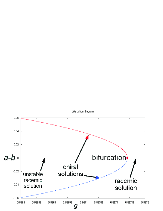
Figure 1: Bifurcation diagram, limited enantioselectivity. For $g>\frac{1-w}{1+3w}$, the unique solution is $y=0$, i.e. $[L]=[D]$, which corresponds to a racemic solution. Reducing $g$ below the critical value, the system undergoes a pitchfork bifurcation, leading to chiral solutions, i.e. $[L]\neq[D]$. This is illustrated here for $g_{crit}=0.85714$ ($w=0.04$). These chiral solutions however are not homochiral, as they yield an enantiomeric excess $ee$ strictly less than unity, provided that $k_{3}\neq 0$; see Eq.(49).

Table 1: Selected reaction schemes treated as open systems, and the corresponding condition $g<g_{crit}$ that must be satisfied for obtaining a stable chiral solution.

Reaction model (open systems: $[A]=$ constant)	$g$	$g_{crit}$	$g<g_{crit}$
Frank (with $k_{1}=k_{-1}=0$)	$\frac{k_{-2}}{k_{5}}$	1	$k_{-2}<k_{5}$
Frank (with $k_{1}>0,\,k_{-1}>0$)	$\frac{k_{-2}}{k_{5}}$	$\frac{1}{8u}(\sqrt{1+16u}-1)$	$\frac{k_{-2}}{k_{5}}<\frac{1}{8u}(\sqrt{1+16u}-1)$
Frank + reversible heterodimers	$\frac{k_{-2}}{k_{5}}$	0	–
Frank + reversible homo- and heterodimers	$\frac{k_{-2}+2k_{4}}{k_{5}}$	$q=\frac{2k_{4}}{k_{5}}$	–
Limited enantioselectivity	$\frac{k_{-2}}{k_{-3}}$	$\frac{1-w}{1+3w}$	$\frac{k_{-2}}{k_{-3}}<\frac{1-w}{1+3w}$
Lim. enantiosel. plus heterodimers	$\frac{k_{-2}}{k_{-3}+k_{5}}$	$(1-s)\frac{1-w}{1+3w}$	$\frac{k_{-2}}{k_{-3}}<\frac{1-w}{1+3w}$
Lim. enantiosel. plus homodimers	$\frac{k_{-2}+2k_{4}}{k_{-3}}$	$\frac{1+q-w+3qw}{1+3w}$	$\frac{k_{-2}}{k_{-3}}<\frac{1-w}{1+3w}$
Lim. enantiosel. plus homo- and heterodimers	$\frac{k_{-2}+2k_{4}}{k_{-3}+k_{5}}$	$\frac{1+q-s-w+3qw+sw}{1+3w}$	$\frac{k_{-2}}{k_{-3}}<\frac{1-w}{1+3w}$

.

IV.5 Limited enantioselectivity plus dimers

It is natural to ask if including dimer formation can alter the symmetry breaking condition $g<g_{crit}$ and get around the thermodynamic constraint. To this end, and for more chemical realism, we include the dimerizations. We begin with just the hetero-dimerization step, and the static solutions work out to be given by

$$O \equiv \big{(}P=0,y=0,\chi=0\big{)}$$ (51)

$$R \equiv \big{(}P=\frac{s(1+w)^{2}}{r(1+g-s)^{2}},y=0,\chi=\frac{2(1+w)}{1+g-s}\big{)}$$ (52)

$$Q_{\pm} \equiv \big{(}P=\frac{s(-1+w)w}{gr(-1+g+s)},y=\pm\frac{\sqrt{1-w}\sqrt{\frac{-1+g+s+w+3gw-sw}{g}}}{\sqrt{g}\sqrt{-1+g+s}},\chi=\frac{1-w}{g}\big{)}$$ (53)

The eigenvalues for the empty and racemic solution can be found in closed form. They are given by

$$\lambda_{1,2,3}(O)=(-r,1-w,1+w).$$ (54)

and

$$\lambda_{1,2,3}(R)=\Big{(}1-w-\frac{2g(1+w)}{1+g-s},$$ (55)

$$- \frac{1+r+s-rs+w+sw+g(1+r+w)}{2(1+g-s)}$$

$$+ \frac{\sqrt{-4r(1+g-s)^{2}(1+w)+(1+r+s-rs+w+sw+g(1+r+w))^{2}}}{2(1+g-s)},$$

$$\frac{r(-1-g+s)-(1+g+s)(1+w)}{2(1+g-s)}$$

$$+ \frac{\sqrt{-4r(1+g-s)^{2}(1+w)+(1+r+s-rs+w+sw+g(1+r+w))^{2}}}{2(1+g-s)}\Big{)}.$$

Note that here, $g=\frac{k_{-2}}{k_{-3}+k_{5}}$. The empty solution $O$ is always unstable. As for the racemic solution $R$, we note that $\lambda_{1}(R)<0$ provided that $g>\frac{(1-s)(1-w)}{1+3w}$. The remaining two eigenvalues $\lambda_{2,3}(R)<0$ for $r>0,w>0,1>s>0$ and for all $g>0$. So the racemic state is stable when $g>g_{crit}=\frac{(1-s)(1-w)}{1+3w}$ and unstable when $g<g_{crit}$. Clearly, when the racemic state is unstable, we infer that chiral state is the only stable solution.

Note that the expression for the critical $g$ in this model is just the $g_{crit}$ for the limited enantioselectivity model treated above times the additional factor $(1-s)$, see Table 1. In other words, the inclusion of heterodimer formation and dissociation seems to reduce the value of $g_{crit}$, appearing to making chiral symmetry breaking relatively more difficult to achieve. But since $s=\frac{k_{5}}{k_{-3}+k_{5}}$, the crucial inequality $g<g_{crit}$ actually reduces algebraically and simplifies to yield the one obtained for the limited enantioselectivity model without heterodimers.

For completeness, we also have worked out the fixed point solutions and their stability properties first, when only the homodimers, and then when both the homo-and heterodimers are included. The results of these latter two cases are summarized in the seventh and eighth rows of Table 1. It is interesting to point out that although the expressions for the critical $g$’s depend on the homo and heterodimer rates explicitly and in a non-trivial way (see the third column), the final inequalities $g<g_{crit}$ determining the stable chiral outcomes are the same as for limited enantioselectivity alone, irrespective of whether the homo and/or heterodimers are included. Compare the fifth and seventh rows of the Table, as well as the sixth and eighth rows. The dependence on $k_{4}$ or $q$ simply cancels out. The inclusion of dimer formation does not affect the symmetry breaking in this model. Since the condition $\frac{k_{1}}{k_{-1}}=\frac{k_{2}}{k_{-2}}=\frac{k_{3}}{k_{-3}}$ continues to hold, only the racemic state is stable.

V Closed reaction systems

For closed systems there is no flow of material into or out of the system. Since $[A]$ is not constant in this situation, we cannot use it to rescale the time or the concentrations. We can however take $\tau=k_{1}t$ for the time and $[\tilde{L}]=\frac{k_{-3}+k_{5}}{k_{1}}[L]$, etc. for the dimensionless concentrations. This allows us to express the rate equations in Sec II in the following dimensionless form:

$$\frac{d}{d\tau}[\tilde{L}] = [\tilde{A}]-u[\tilde{L}]+h[\tilde{A}][\tilde{L}]-g[\tilde{L}]^{2}-[\tilde{L}][\tilde{D}]+r[\tilde{A}][\tilde{D}]+2\omega[\tilde{L}_{2}]+\rho[\tilde{LD}],$$

$$\frac{d}{d\tau}[\tilde{D}] = [\tilde{A}]-u[\tilde{D}]+h[\tilde{A}][\tilde{D}]-g[\tilde{D}]^{2}-[\tilde{D}][\tilde{L}]+r[\tilde{A}][\tilde{L}]+2\omega[\tilde{D}_{2}]+\rho[\tilde{LD}],$$

$$\frac{d}{d\tau}[\tilde{L}_{2}] = \frac{q}{2}[\tilde{L}]^{2}-\omega[\tilde{L}_{2}],$$

$$\frac{d}{d\tau}[\tilde{D}_{2}] = \frac{q}{2}[\tilde{D}]^{2}-\omega[\tilde{D}_{2}],$$

$$\frac{d}{d\tau}[\tilde{LD}] = s[\tilde{L}][\tilde{D}]-\rho[\tilde{LD}].$$

These are subject to the constraint $[\tilde{A}]=C-[\tilde{L}]-[\tilde{D}]-2[\tilde{L}_{2}]-2[\tilde{D}_{2}]-2[\tilde{LD}]$, where $C$ is a constant. The parameters appearing here are

$$u = \frac{k_{-1}}{k_{1}},\,g=\frac{k_{-2}+2k_{4}}{k_{-3}+k_{5}},\,h=\frac{k_{2}}{k_{-3}+k_{5}},\,r=\frac{k_{3}}{k_{-3}+k_{5}},\,\rho=\frac{k_{-5}}{k_{1}},\,\omega=\frac{k_{-4}}{k_{1}},\,q=\frac{2k_{4}}{k_{-3}+k_{5}},$$ (56)

$${\rm and} \,s=\frac{k_{5}}{(k_{-3}+k_{5})}.$$

For closed systems, the number of independent parameters reduces from ten to eight.

As before, we find it convenient to define the sums and differences of concentrations: $\chi=[\tilde{L}]+[\tilde{D}]$, $y=[\tilde{L}]-[\tilde{D}]$, $\chi_{2}=[\tilde{L}_{2}]+[\tilde{D}_{2}]$ $y_{2}=[\tilde{L}_{2}]-[\tilde{D}_{2}]$, and put $P=[\tilde{LD}]$. This then yields the following:

$$\frac{d}{d\tau}\chi = 2[\tilde{A}]+((h+r)[\tilde{A}]-u)\chi-\frac{1}{2}(g+1)\chi^{2}-\frac{1}{2}(g-1)y^{2}+2\omega\,\chi_{2}+2\rho\,P,$$ (57)

$$\frac{d}{d\tau}y = y\big{(}(h-r)[\tilde{A}]-g\chi-u\big{)}+2\omega\,y_{2},$$ (58)

$$\frac{d}{d\tau}\chi_{2} = \frac{q}{4}(\chi^{2}+y^{2})-\omega\,\chi_{2},$$ (59)

$$\frac{d}{d\tau}y_{2} = \frac{q}{2}\chi y-\omega\,y_{2},$$ (60)

$$\frac{d}{d\tau}P = \frac{s}{4}(\chi^{2}-y^{2})-\rho P.$$ (61)

In these variables, the constant mass constraint reads $[\tilde{A}]=C-\chi-2\chi_{2}-2P$.

For the complete closed model, that is, the reaction steps in Eqs.(1-5), the $5\times 5$ Jacobian matrix $M_{closed}$ for the linearized fluctuation equations is given by

$$M_{closed}=\left(\begin{array}[]{ccccc}\scriptstyle{(h+r)(C-2\chi_{2}-2P)-(2+u)}&\scriptstyle{(1-g)y}&\scriptstyle{2\omega-4-2(h+r)\chi}&0&\scriptstyle{2\rho-4-2(h+r)\chi}\\ \scriptstyle{-(g+1+2(h+r))\chi}&&&&\\ &&&&\\ \scriptstyle{-(g+h-r)y}&\scriptstyle{(h-r)(C-2\chi_{2}-2P)}&\scriptstyle{-2(h-r)y}&\scriptstyle{2\omega}&\scriptstyle{-2(h-r)y}\\ &\scriptstyle{-(g+h-r)\chi-u}&&&\\ &&&&\\ \frac{q}{2}\chi&\frac{q}{2}y&-\omega&0&0\\ \frac{q}{2}y&\frac{q}{2}\chi&0&-\omega&0\\ \frac{s}{2}\chi&-\frac{s}{2}y&0&0&-\rho\\ \end{array}\right).$$ (62)

This incorporates the constraint equation directly. This matrix is to be evaluated on any of the static fixed point solutions $\chi^{*},y^{*},\chi^{*}_{2},y^{*}_{2}$ and $P^{*}$ of the equation set Eqs.(57-61). The constant $C$ is related to the total initial concentration $Q$ as follows: $C=\frac{k_{-3}+k_{5}}{k_{1}}Q$. The eigenvalues of $M_{closed}$ indicate the stability of the static solution on which this matrix is evaluated. Unlike the open flow case however, it is much more difficult to obtain manageable analytic expressions for these eigenvalues, and the variety of reaction schemes we can treat analytically in this manner is limited.

V.1 Closed Frank with irreversible heterodimers: $k_{-5}=0$

Recall that the Frank model in an open flow system and with irreversible formation of heterodimers does lead to stable steady-state chiral solutions. We now enclose it in a box, so that $[A]$ is no longer constant. In this situation we are to solve the Eqs.(57,58,61) where from the parameter list in Eq(56) we have $u>0$, $g=k_{-2}/k_{5}$, $h=k_{2}/k_{5}$, $r=\omega=q=0$, $s=1$ and for $k_{-5}=0$, we must set $\rho=0$. The mass constraint reads $[\tilde{A}]=C-\chi-2P$. There is a static racemic $R$ and two static chiral $Q_{\pm}$ solutions:

$$\begin{array}[]{lll}R&\equiv(P=\frac{C}{2},y=0,\chi=0)\\ Q_{\pm}&\equiv\left(P=\frac{Cg+u}{2g},y=\pm\frac{u}{g},\chi=-\frac{u}{g}\right).\end{array}$$ (65)

Note that the chiral solutions are unphysical since they imply $\chi<0$ when $u>0$. We can attempt to get some information regarding stability by evaluating the $3\times 3$ array obtained from Eq.(62) after deleting the 3rd and 4rth rows and columns. The eigenvalues corresponding to the racemic solution are

$$\lambda_{1,2,3}(R)=(0,-2-u,-u),$$ (66)

indicating that $R$ is marginally stable (marginal because of the zero entry). We are unable to calculate the eigenvalues for the unphysical chiral states in simple analytic form. For $u=0$, the only steady state is the racemic one $R$, (there is no steady chiral solution) and its eigenvalue is (0,-2,0).

This is important, because Model 1 of Rivera Islas et al Islas , is actually a special case of this, in which $u=g=0$, and we consider this next.

V.2 Rivera Islas et. al. Model 1

This model Islas corresponds to our reaction steps Eqs(1,2,5) and after setting $k_{-1}=k_{-2}=k_{-5}=0$. Note this model implies irreversible reactions. This is a closed system, we we solve again the Eqs.(57,58,61) where from the parameter list in Eq(56), we now have $u=0$, $g=0$, $h=k_{2}/k_{5}$, $r=\omega=q=0$, $s=1$ and for $k_{-5}=0$, we must set $\rho=0$. The constraint is $[\tilde{A}]=C-\chi-2P$. We next look for the static solutions of the set of equations Eqs.(57,58,61). The racemic solution $y=0$ implies that $\chi=0$ and $P=C/2$. Thus, all the net matter ends up as heterodimers. On the other hand, the chiral solution has $y\neq 0$. For this case, the static solution of Eqs.(57,58,61) yields $\chi^{2}=y^{2}$ and $C-2P=\chi$. The physical solution corresponds to a positive $\chi>0$, so that $y=\pm\chi$ and $P=\frac{C-\chi}{2}>0$. In this case, the total matter is distributed among monomers and dimers. Note however we cannot independently solve for the final heterodimer and monomer concentration in the chiral phase. The static solutions are summarized as follows:

$$\begin{array}[]{lll}R&\equiv(P=\frac{C}{2},y=0,\chi=0)\\ Q_{\pm}&\equiv\left(P=\frac{C-\chi}{2},y=\pm\chi\right).\end{array}$$ (69)

Using $M_{closed}$ to compute the eigenvalues for this case, we find that

$${\lambda_{1,2,3}(R)}_{Islas}=(-2,0,0).$$ (70)

Since ${\lambda_{2,3}(R)}_{Islas}=0$, we cannot say conclusively if this state is stable or unstable. This is in accord with the chemical fact that due to its irreversibility, this reaction scheme leads to a kinetic controlled outcome of the reaction products. Evaluating Eq.(62) on this chiral solution and calculating the eigenvalues yields

$${\lambda_{1,2,3}(Q)}_{Islas}=(0,-\chi,-2-h\chi).$$ (71)

This is as much as we can say regarding linear stability analysis; there are no free adjustable parameters that can induce a change in sign in any of the eigenvalues. The simple stability analysis is inconclusive. Nevertheless, numerical simulations carried out in Islas indicate stable chirally asymmetric solutions for a range of $h$. Thus, a higher order stability analysis might be called for.

V.3 Limited enantioselectivity revisited: the closed system

We can obtain the static solutions and their associated eigenvalues exactly for limited enantioselectivity in a closed system, the model introduced in Subsection IV.4. This is useful because it provides an exact point of comparison between a specific set of reactions in both open and closed systems. So we consider the reaction set Eqs.(1,2,3), but now in a closed system. We must solve Eqs.(57,58) in which we set $\chi_{2}=P=y_{2}=0$. The mass constraint in this case reads $[\tilde{A}]=C-\chi$. There are four static solutions (note we also set $u=0$ to simplify somewhat the algebra):

$$U\equiv\big{(}y = 0,\,\chi=-\frac{2-C(h+r)+\sqrt{4C(1+g+2(h+r))+(2-C(h+r))^{2}}}{1+g+2(h+r)}\big{)}\$$ (72)

$$R\equiv\big{(}y = 0,\,\chi=\frac{-2+C(h+r)+\sqrt{4C(1+g+2(h+r))+(2-C(h+r))^{2}}}{1+g+2(h+r)}\big{)}\$$ (73)

$$Q_{\pm}\equiv\big{(}y = \pm\sqrt{\frac{4Cg(g+h-r)+C^{2}(h-r)((-1+g)h+r+3gr)}{(g-1)(g+h-r)^{2}}},\,\chi=\frac{C(h-r)}{g+h-r}\big{)}.$$ (74)

$U$ denotes the unphysical solution, as this implies a negative total chiral matter, $R$ is the racemic solution with positive net total chiral matter, and $Q_{\pm}$ denote the two possible chiral solutions. Note from Eq.(56) we have $g=\frac{k_{-2}}{k_{-3}},\,h=\frac{k_{2}}{k_{-3}},\,r=\frac{k_{3}}{k_{-3}}$.

The stability of the four possible homogeneous solutions $U,R$ and $Q_{\pm}$, is determined from considering the eigenvalues of the $2\times 2$ subblock of the upper left hand corner of the Jacobian matrix $M_{closed}$ Eq.(62) (and after setting $\chi_{2}=P=0$ as well as $u=0$) evaluated at each one of these four possible solutions. The eigenvalues are given by

$$\lambda_{1,2}(U) = \Big{(}C(h-r)-\frac{(g+h-r)}{1+g+2h+2r}\left(-2+C(h+r)-\sqrt{4+C^{2}(h+r)^{2}+4C(1+g+h+r)}\right),$$ (75)

$$\sqrt{4+C^{2}(h+r)^{2}+4C(1+g+h+r)}\Big{)}$$

$$\lambda_{1,2}(R) = \Big{(}C(h-r)-\frac{(g+h-r)}{1+g+2h+2r}\left(-2+C(h+r)+\sqrt{4+C^{2}(h+r)^{2}+4C(1+g+h+r)}\right),$$ (76)

$$- \sqrt{4+C^{2}(h+r)^{2}+4C(1+g+h+r)}\Big{)}$$

and

$$\lambda_{1,2}(Q_{\pm}) = \frac{1}{2(g+h-r)}(2g(-1+Cr)+(-h+r)(2+C(1+h+r))$$

$$+ \surd((g(2-2Cr)+(h-r)(2+C(1+h+r)))^{2}$$

$$+ 4C(g+h-r)(4g^{2}-C(h-r)^{2}+g(h-r)(4+C(h+3r))))),$$

$$\frac{1}{2(g+h-r)}(2g(-1+Cr)+(-h+r)(2+C(1+h+r))$$

$$- \surd((g(2-2Cr)+(h-r)(2+C(1+h+r)))^{2}$$

$$+ 4C(g+h-r)(4g^{2}-C(h-r)^{2}+g(h-r)(4+C(h+3r)))))$$

As $\lambda_{2}(U)>0$, the unphysical solution $U$ is therefore always unstable. To ensure the stability in $R$, we need for both eigenvalues to be negative: $\lambda_{1,2}(R)<0$. While the second eigenvalue is always negative, we have $\lambda_{1}(R)<0$ if and only if $g>g_{crit}$, where

$$g_{crit}=-\frac{1}{8}(h-r)\left(4+C(h+3r)-\sqrt{16+C^{2}(h+3r)^{2}+8C(2+h+3r)}\right).$$ (77)

A careful expansion of this shows that in the limit of large $C$, then the critical value of $g$

$$g_{crit}\rightarrow\frac{1-r/h}{1+3r/h}=\frac{1-k_{3}/k_{2}}{1+3k_{3}/k_{2}}=\frac{1-w}{1+3w}=g_{crit}^{open},$$ (78)

asymptotically approaches the critical $g$ for the same set of reactions in an open system, Eq.(50).

Concerning the stability of the solutions $Q_{\pm}$, these are always unstable if $g>1$ and they become stable $\lambda_{1,2}(Q_{\pm})<0$ for $0<g<g_{crit}<1$. However, the thermodynamic condition mentioned above still holds and implies that the racemic state is the only stable outcome.

VI Concluding remarks

We have focussed attention on the steady state solutions and their dynamic stability properties in variants of both the Frank and limited enantioselectivity models of mirror symmetry breaking. In the Frank model Frank ; Mason , the mutual inhibition occurs through the formation of heterodimers composed of the two chiral monomers, whereas in limited enantioselectivity Avet ; GH , the needed chiral antagonism occurs though a monomer recycling reaction. We have unified both models into one encompassing reaction scheme and have studied the steady state solutions and their stability properties in a sequence of reaction schemes that start from the paradigmatic Frank model to limited enantioselectivity, in which we study the consequences of including the formation of (reversible) hetero- and homo-dimers as dynamic variable concentrations in both. The general conclusion we can draw from this is that the inclusion of the variable heterodimer concentrations leads to a final stable racemic state in the sequence of Frank-type models defined above. This is important because we recall that in Frank’s original formulation, the heterodimers are supposed to be removed from the system, i.e., their formation is irreversible. Including the homodimers does not affect this conclusion.

In the case of the limited enantioselectivity model, no dimer formation is originally contemplated, and mirror symmetry breaking is mathematically possible because the needed inhibition is provided by the reverse symmetric catalysis step GH . In spite of this, the symmetry breaking condition $g<g_{crit}$, determined from the pure stability analysis, cannot be achieved on thermodynamic grounds GH , as has also been pointed out recently Matar . Including the homo- and/or the heterodimer formation to limited enantioselectivity does not alter the crucial inequality, nor does the presence of the dimers change the thermodynamic constraint. Therefore an open question is if a different chemical scenario leading to collective phenomena exists, such as a second order phase transition, that can give rise to the condition $g<g_{crit}$. In the context of spatially extended polymerization systems, it has been argued before that one should expect domain formation similar to the case of second order phase transitions BM ; Gleiser ; GW .

The reaction networks treated here are limited to reactions involving only monomers and dimers, whereas biological chirality of living systems involves large macromolecules that are probably the result of polimerization reactions. In this vein, Sandars recently introduced a model in which the detailed polymerization process and enantiomeric cross-inhibition are taken into account, its basic features are explored numerically, but without including spatial extent, chiral bias or noise Sandars . Brandenburg and coworkers have analyzed further properties of Sandars’ model and have proposed a truncated version including chiral bias BAHN , and have studied this reduction with spatial extent and coupling to a turbulent advection velocity BM . Gleiser and Thorarinson analyze the reduced Sandars’ model with spatial extent and coupling to an external white noise GT and in Gleiser , Gleiser considers the reduced chiral biased model with external noise. In addition to Sandars, both Wattis and Coveney Wattis and Saito and Hyuga Saito have introduced polymerization models that can give rise to homochiral states. The latter one differs from Sandars’ in allowing for reversibility in all the steps. As reported in the review article (d) in all , all these polymerization models derive from Frank’s model by adding polymerization reactions. Thus, in spite of the simplicity of the original Frank model Frank , ignoring as it does the polymerization process, it continues to serve as a type of “Ising model” for chiral symmetry breaking.

- (1) a) K. Soai, T. Shibata, H. Morioka and K. Choji, Nature 378, 767-768 (1995). b) K. Soai, I. Sato, T. Shibata, S. Komiya, M. Hayashi, Y. Matsueda, H. Imamura, T. Hayase, H. Moioka, H. Tabira, J. Yamamoto and Y. Kowata, Tetrahedron: Asymmetry 14, 185-188 (2003). c) I.D. Gridnev, J.M. Serafimov, H. Quiney and J.M. Brown, Org. Biomol. Chem. 1, 3811-3819 (2003). d) T. Kawasaki, K. Jo, H. Igarashi, I. Sato, M. Nagano, H. Koshima and K. Soai, Angew. Chem. Int. Ed. 44, 2774-2777 (2005). e) T. Kawasaki, K. Suzuki, M. Shimizu, K. Ishikawa and K. Soai, Chirality 18, 479-482 (2006).
- (2) C. Viedma, Phys. Rev. Lett. 94, 065504 (2005).
- (3) M. Mauksch, S.B. Tsogoeva, I.M. Martynova and S. Wei, Angew. Chem. Int. Ed. 46, 393-396 (2007). M. Mauksch, S.B. Tsogoeva, S. Wei and I.M. Martynova, Chirality 19, 816-825 (2007).
- (4) W.L. Noorduin, T. Izumi, A. Millemaggi, M. Leeman, H. Meekes, W.J.P. Van Enckevort, R.M. Kellogg, B. Kaptein, E. Vlieg, and D.G. Blackmond, J. Am. Chem. Soc. 130, 1158-1159 (2008).
- (5) For the most rigorous definition of absolute asymmetric synthesis, see L. Caglioti, C. Hajdu, O. Holczknecht, L. Zekany, C. Zucchi, K. Micskei, G. Palyi, Viva Origino 34, 62 (2006).
- (6) J. Crusats, S. Veintemillas-Verdaguer and J.M. Ribo, Chem. Eur. J. 12, 7567 (2006).
- (7) F.C. Frank, Biochim. et Biophys. Acta 11, 459 (1953).
- (8) J. Rivera Islas, D. Lavabre, J.-M. Grevy, R. Hernández Lamoneda, H. Rojas Cabrera, J.-C. Micheau and T. Buhse, Proc. Natl. Acad. Sci. USA 102, 13743 (2005).
- (9) a) D.G. Blackmond, Proc. Natl. Acad. Sci. U.S.A. 101, 5732 (2004), : b) K.D. Kondepudi and K. Asakura, Acc. Chem. Res. 124, 946-954 (2001). c) K. Mikami and M. Yamanaka, Chem. Rev. 103, 3369-3400 (2003). d) R. Plasson, D.K. Kondepudi, H. Bersini, A. Commeyras and K. Asakura, Chirality 19, 589-600 (2007); R. Plasson, H. Bersini, A. Commeyras, Proc. Natl. Acad. Sci. U.S.A., 101, 16733 (2004)
- (10) A.R. Hochstim, Orig. Life. 6, 317 (1975).
- (11) S.F. Mason, Chemical Evolution (Oxford University Press, Oxford, 1991).
- (12) S.F. Mason, Nature 314, 400 (1985).
- (13) V. Avetisov and V. Goldanskii, Proc. Natl. Acad. Sci. USA 93, 11435 (1996).
- (14) W.H. Mills, Chem. Ind. (London), 750 (1932).
- (15) G. Lente, J. Phys. Chem. A 108, 9475 (2004).
- (16) D. Hochberg and M.-P. Zorzano, Chem. Phys. Lett. 431, 185 (2006).
- (17) D. Hochberg and M.-P. Zorzano, Phys. Rev. E76, 021109 (2007).
- (18) G. Palyi, C. Zucchi, L. Caglioti (Eds) Advances in BioChirality (Elsevier, Amsterdam, 1999); G. Palyi, C. Zucchi, L. Caglioti (Eds) Progress in Biological Chirality (Elsevier, Oxford, 2004).
- (19) M. Eigen, Naturwiss. 58, 465 (1971), T. Ganti, Bio Systems 7 , 15 (1975).
- (20) M. Quack, Angew. Chem., Int. Ed. 41, 4618 (2002).
- (21) I. Gutman, D. Todorović and M. Vučković, Chem. Phys. Lett. 216, 447 (1993).
- (22) S.W. Benson, The Foundations of Chemical Kinetics (McGraw-Hill, New York, 1960).
- (23) R. Chang, Physical Chemistry (University Science Books, Sausalito, 2000).
- (24) A. Giaquinta and D. Hochberg, Physica D 237, 2563 (2008).
- (25) G. Lebon, D. Jou and J. Casas-Vazquez, Understanding non-equilibrium thermodynamics (Springer, Berlin, 2008) pp 97-98.
- (26) D.G. Blackmond and O.K. Matar, J. Phys. Chem. B 112, 5098 (2008).
- (27) A. Brandenburg and T. Multamäki, Int. J. Astrobiol. 3, 209 (2004).
- (28) M. Gleiser, Orig. Life Evol. Biosph. 37, 235 (2007).
- (29) M. Gleiser and S.I. Walker, Orig. Life Evol. Biosph. 38, 293 (2008).
- (30) P.G.H. Sandars, Orig. Life Evol. Biosph. 33, 575 (2003).
- (31) A. Brandenburg, A.C. Andersen, S. Höfner and M. Nilsson, Orig. Life Evol. Biosph. 35, 225 (2005).
- (32) M. Gleiser and J. Thorarinson, Orig. Life Evol. Biosph. 36, 501 (2006).
- (33) J.A. Wattis and P.V. Coveney, Orig. Life Evol. Biosph. 35, 243 (2005).
- (34) Y. Saito and Hyuga, J Phys Soc Jpn 74, 1629 (2005).