The [O II] $\lambda 3727$ Luminosity Function at $z\sim 1$

Abstract

We measure the evolution of the [O II] $\lambda 3727$ luminosity function at $0.75<z<1.45$ using high-resolution spectroscopy of $\sim 14,000$ galaxies observed by the DEEP2 galaxy redshift survey. We find that brighter than $L_{\mathrm{[OII]}}=10^{42}~{}\mathrm{erg~{}s^{-1}}$ the luminosity function is well-represented by a power law $dN/dL\propto L^{\alpha}$ with slope $\alpha\sim-3$. The number density of [O II]-emitting galaxies above this luminosity declines by a factor of $\gtrsim 2.5$ between $z\sim 1.35$ and $z\sim 0.84$. In the limit of no number-density evolution, the characteristic [O II] luminosity, $L_{\mathrm{[OII]}}^{*}$, defined as the luminosity where the space density equals $10^{-3.5}~{}\mathrm{dex^{-1}~{}Mpc^{-3}}$, declines by a factor of $\sim 1.8$ over the same redshift interval. Assuming that $L_{\mathrm{[OII]}}$ is proportional to the star-formation rate (SFR), and negligible change in the typical dust attenuation in galaxies at fixed [O II] luminosity, the measured decline in $L_{\mathrm{[OII]}}^{*}$ implies a $\sim 25\%$ per Gyr decrease in the amount of star formation in galaxies during this epoch. Adopting a faint-end power-law slope of $-1.3\pm 0.2$, we derive the comoving SFR density in four redshift bins centered around $z\sim 1$ by integrating the observed [O II] luminosity function using a local, empirical calibration between $L_{\mathrm{[OII]}}$ and SFR, which statistically accounts for variations in dust attenuation and metallicity among galaxies. We find that our estimate of the SFR density at $z\sim 1$ is consistent with previous measurements based on a variety of independent SFR indicators.

1. Introduction

Measuring the comoving space density of the star formation rate (SFR) as a function of cosmic epoch is one of the key issues concerning the study of galaxy formation and evolution. The current picture is that the star formation peaked at $z\sim 1-3$, and then declined by roughly an order-of-magnitude to the present day (see, e.g., Madau et al. 1996; Lilly et al. 1996; Hopkins 2004; Hopkins & Beacom 2006).

Among the most direct indicators of the instantaneous SFR in galaxies is the H$\alpha$ $\lambda 6563$ recombination line (Kennicutt 1983, 1992). H$\alpha$ can be observed in the optical in the local Universe (e.g., Gallego et al. 1995; Tresse et al. 1998; Kennicutt 2008). However, at $z\gtrsim 0.4$, it must be observed in the near infrared (e.g., Yan et al. 1999; Glazebrook et al. 1999; Hopkins et al. 2000; Tresse et al. 2002), or other less direct SFR indicators such as the [O II] $\lambda\lambda 3726,3729$ doublet must be used.

Compared to H$\alpha$, [O II] is only indirectly coupled to the ionizing continuum from massive stars, and is more sensitive to variations in metal abundance, excitation, and dust attenuation. Nevertheless, because of its intrinsic strength and blue rest-frame wavelength, [O II] remains a good alternative SFR indicator for high-redshift galaxies (Kennicutt 1998; Jansen et al. 2001; Kewley et al. 2004; Mouhcine et al. 2005; Moustakas & Kennicutt 2006). In the past decade, a number of investigators have measured the star formation rate density, $\rho_{\rm SFR}$, at high redshift by studying the [O II] luminosity function (LF), either using spectroscopy (e.g., Hammer et al. 1997; Hogg et al. 1998; Gallego et al. 2002; Teplitz et al. 2003; Rigopoulou et al. 2005), or narrow-band imaging (e.g., Hippelein et al. 2003; Ly et al. 2007, hereafter Ly07; Takahashi et al. 2007, hereafter Takahashi07). Unfortunately, these studies have been hampered by small sample size, small volume probed, and an inconsistent treatment of dust obscuration. Methods like narrow-band imaging also suffer from difficulties in continuum subtraction and contamination from other emission lines.

To circumvent these issues, we measure the [O II] luminosity function at $z\sim 1$ using data from the Deep Extragalactic Evolutionary Probe 2 survey (DEEP2; Davis et al. 2003). DEEP2 has obtained high-resolution spectra for $\sim 50,000$ objects over four separate fields, making it the largest existing spectroscopic redshift survey of galaxies at these redshifts. We use these data to measure the [O II] luminosity function in four redshift bins at $0.75<z<1.45$.

In $\S$2, we briefly describe our sample and the method used to calculate the LF. In §3 and §4 we present the observed [O II] LF and its evolution with redshift, respectively. Finally, in $\S$5, we compute $\rho_{\rm SFR}$ in several redshift bins centered around $z\sim 1$, and we summarize our principal conclusions in $\S$6.

Throughout this work, we adopt a $\Lambda\mathrm{CDM}$ cosmology with $\Omega_{\mathrm{m}}=0.3$, $\Omega_{\Lambda}=0.7$ and $H_{0}=70~{}\mathrm{km~{}s^{-1}~{}Mpc^{-1}}$. All magnitudes are on the AB system.

2. Data and Method

2.1. Data: DEEP2 DR3

We select our sample from the DEEP2 third public data release (DR3), which includes $BRI$ photometry and spectra for $\sim 50,000$ galaxies in four widely separated fields. The high-resolution ($R\equiv\lambda/\delta\lambda\sim 5000$) spectra, which were acquired using the Keck-II/DEIMOS spectrograph (Faber et al., 2003), span $6525-9120$ Å. We thus restrict our analysis to the redshift range $0.75<z<1.45$, where [O II] is measurable. To study the evolution of the [O II]  LF, we further split each bin into four additional redshift bins: $0.75<z<0.93$; $0.93<z<1.10$; $1.10<z<1.28$; and $1.28<z<1.45$. We refer the reader to Davis et al. (2003), Coil et al. (2004), and Davis et al. (2007) for additional details regarding the DEEP2 survey.

In addition to the flux cut, $R<24.1$ mag, the DEEP2 team applied the following color cuts to preselect galaxies at $z>0.7$ in Fields 2, 3, and 4:

$$B-R < 2.35(R-I)-0.25\ {\rm or};$$

$$R-I > 1.15\ {\rm or};$$

$$B-R < 0.50.$$ (1)

In the Extended Groth Strip (EGS, Field 1), to test their sample preselection method, the DEEP2 team did not apply the $BRI$ color cuts. However, in order to make all four fields consistent, here we apply the color cuts given by equation (1) to the redshift and photometric catalogs in the EGS field. We apply additional angular cuts to avoid survey edges and to exclude gaps in the spectroscopy. Our final catalog contains $36,118$ objects, of which $24,729$ have accurate redshifts (quality $Q=3$ or $4$ as defined by Davis et al. 2007). The areas of the four fields are $0.38$, $0.56$, $0.88$ and $0.63~{}\mathrm{deg}^{2}$, respectively, and the total area is $2.45~{}\mathrm{deg}^{2}$.

Next we describe how we derive the integrated [O II] luminosity for each galaxy. Unfortunately, the DEEP2 spectra are not flux-calibrated; therefore we infer the [O II] luminosity by multiplying the rest-frame emission-line equivalent width (EW) measured in the optical spectra, by the continuum luminosity around $3727$ Å inferred from fitting the $BRI$ photometry. This method has the advantage that it is insensitive to the absolute calibration of the optical spectra. However, the $1\arcsec$ wide slit in the DEEP2 survey may not enclose all the line-emitting regions in the galaxy, thus this method does assume that the relative intensity of star formation and stellar light inside and outside the slit does not vary significantly. Without spatially resolved spectroscopy, however, this assumption is difficult to test directly.

To measure the emission-line EW, we model each component of the [O II] $\lambda\lambda 3726,3729$ doublet simultaneously using two Gaussian profiles, constrained to have the same intrinsic velocity width and a fixed wavelength separation, and use a smooth $B$-spline to estimate the continuum level around [O II]. Dividing the total [O II] flux by the detected continuum yields the rest-frame EW([O II]) in Å. We then fit the broad-band $BRI$ photometry at the known redshift to obtain the best-fitting spectral energy distribution (SED) using the deep_kcorrect routine in kcorrect (v4.1.4; Blanton & Roweis 2007). Finally, we multiply the EW by the flux-density of the best-fitting SED at $3727$ Å to obtain the integrated [O II] luminosity. Because the effective wavelengths of all the $BRI$ filter bandpasses lie blueward of $3700$ Å above $z\sim 1.2$, this technique does require extrapolating the best-fitting SED beyond the effective $I$-band wavelength to estimate the $3727$ Å continuum luminosity for the galaxies in our highest redshift bin; however, the uncertainty introduced by this extrapolation is negligible.

Our [O II] measurement technique is similar to that used by the DEEP2 team (Weiner et al. 2007; Cooper et al. 2008), although the procedures used to compute $K$-corrections are totally independent. A comparison of our measurements shows no systematic differences and a $\sim 25\%$ scatter, which is comparable to the typical measurement error. We also checked our work by replacing our measurements with theirs, and obtained consistent results. In the following analysis we use our measurements.

We consider an [O II] measurement with signal to noise ratio ($S/N$) larger than $5$ as reliable. In detail, our results are not sensitive to the specific $S/N$ cut used since it only affects weak [O II] detections, for which we are incomplete anyway. For example, using $S/N>2$ has no significant effect on our conclusions. Our final sample of [O II]-emitting galaxies contains $13,944$ objects.

2.2. Method: $1/V_{\mathrm{max}}$ Method

To calculate the luminosity function, we use the non-parametric $1/V_{\mathrm{max}}$ method (Felten, 1976). For a given galaxy, we calculate:

$$V_{\mathrm{max}}=\frac{1}{3}\int d\Omega\int_{z_{\mathrm{min}}}^{z_{\mathrm{max}}}dz\frac{d[D_{c}(z)^{3}]}{dz}f(z)\mathrm{,}$$ (2)

which is suitable for a spatially flat universe. The angular integral is limited to the DEEP2 area, $D_{c}(z)$ is the comoving distance as defined by Hogg (1999), and $f(z)$ expresses the probability of selecting each galaxy in our sample. We assume that $f(z)$ is given by the product of four quantities: $f=f_{\mathrm{target}}\times f_{\mathrm{success}}\times f_{\mathrm{cover}}\times f_{\mathrm{cut}}$, where $f_{\mathrm{target}}$ is the rate at which a source of a given $R$-band magnitude and $B-R$ and $R-I$ color was targeted [see eq. (1)], $f_{\mathrm{success}}$ is the rate at which a redshift was successfully measured, $f_{\mathrm{cover}}$ is the fraction of DEEP2 spectra where the wavelength coverage includes the redshifted [O II] line, and $f_{\mathrm{cut}}$ is a step function, which we determined using the $BRI$ magnitudes and the [O II] $S/N$, as described below. We experimented with including the galaxy surface brightness as a fifth variable in the completeness function (see, e.g., Lin et al. 2008), but found that it did not significantly affect our measured LFs.

For a given galaxy, we calculate $V_{\mathrm{max}}$ using a Monte Carlo method (see Blanton 2006). We randomly choose 1200 values of redshift $z$ between $z_{\mathrm{min}}$ and $z_{\mathrm{max}}$, uniformly distributed in volume. For each redshift, we calculate what the magnitudes of the object would be using deep_kcorrect. To estimate the [O II] $S/N$ at each mock redshift, we first determine the mean noise spectrum for every DEEP2 mask. Then, for a given galaxy, we randomly choose a mask and the corresponding noise spectrum and compare the noise at the actual observed wavelength of [O II] to that at the simulated wavelength as if the galaxy were at the simulated redshift, and obtain the new $S/N$. We then apply the appropriate flux cut, color cuts, [O II] $S/N$ cut and the completeness function to determine the fraction of mock sources that would have passed our selection criteria. Finally, $V_{\mathrm{max}}$ is given by the comoving volume multiplied by this fraction.

When determining the completeness function, we assume a $100\%$ redshift success rate for blue galaxies; that is, we assume that the only targeted blue galaxies without successfully measured redshifts are those for which [O II]  falls outside the wavelength range of the spectra, and thus outside the redshift range studied here. Here, we define blue galaxies using the same definition as Willmer et al. (2006), who also made the same assumption regarding blue galaxies without well-measured redshifts. This assumption is especially reasonable in our analysis because a well-detected [O II] doublet will always result in a well-measured redshift. Finally, we tested our completeness function by calculating the $B$-band LF for all galaxies and comparing with Willmer et al. (2006), and found excellent statistical agreement, and no systematic differences.

3. The Observed [O II] Luminosity Function

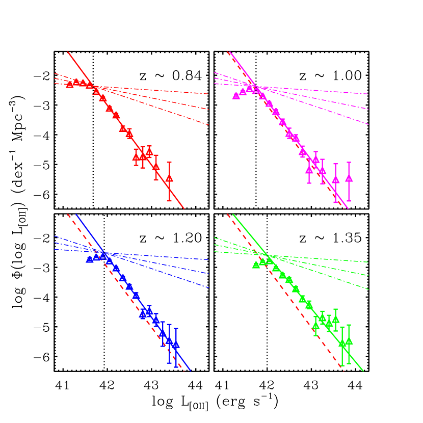
Figure 1.— Observed [O II] luminosity function in four redshift bins. The solid lines are the power-law fits to the bright part of the luminosity function. The dashed lines in the three highest redshift bins correspond to the solid line in the top-left panel. The three dashed-dotted lines correspond to three different faint-end slopes, $-1.1$, $-1.3$ and $-1.5$, and the dotted lines in each panel indicate the turnover in the luminosity function.

We measure the [O II] luminosity function in four redshift bins: $0.75<z<0.93$; $0.93<z<1.10$; $1.10<z<1.28$; and $1.28<z<1.45$, according to where the [O II] doublet could be measured reliably in the DEEP2 spectra. The median redshifts of the [O II]-emitting galaxies within these four redshift bins are $0.84$, $1.01$, $1.19$, and $1.35$, containing $5471$, $3771$, $3018$ and $1684$ galaxies in each bin, respectively.

The resulting [O II] LFs are tabulated in Table 1 and illustrated in Figure 1. The error bars shown in the figure are $84.13\%$ confidence Poisson upper limits and lower limits estimated using the approximate formulas given by Gehrels (1986) [see eqs. (10) and (14) in that paper]. The distribution of the LF must follow a scaled Poisson distribution. To determine the scaling factor, within each luminosity bin, we define the effective weight ($W_{\mathrm{eff}}$) by:

$$W_{\mathrm{eff}}=\left[\sum_{i}{\frac{1}{(V_{\mathrm{max}})^{2}_{i}}}\right]\left/\left[{\sum_{i}{\frac{1}{(V_{\mathrm{max}})_{i}}}}\right]\right.~{}\mathrm{,}$$ (3)

and the effective number ($N_{\mathrm{eff}}$) of objects by:

$$N_{\mathrm{eff}}=\left[\sum_{i}{\frac{1}{(V_{\mathrm{max}})_{i}}}\right]\left/{W_{\mathrm{eff}}}\right.~{}\mathrm{.}$$ (4)

We then calculate the upper limit and lower limit for the effective number, and multiply them by the effective weight to obtain the upper limit and lower limit for the luminosity density in each bin. For comparison, the square root Poisson error gives:

$$\sigma_{\Phi}=\sqrt{N_{\mathrm{eff}}}W_{\mathrm{eff}}=\sqrt{\sum_{i}\frac{1}{(V_{\mathrm{max}})^{2}_{i}}}~{}\mathrm{,}$$ (5)

which is commonly used in the literature. The Poisson errors, however, do not include the effects of cosmic variance. Because we have four widely separated fields, we determine the error due to cosmic variance, $\sigma_{\mathrm{cv}}$, by calculating the variance among the four independent fields, and list the results in Table 1.

Examining Figure 1, the commonly used Schechter (1976) function is clearly a poor representation of the data. Instead, we model the observed [O II] LF in each redshift bin as a power law:

$$\Phi(\log L)d(\log L)=10^{(\alpha+1)(\log L-42.5)+\beta}d(\log L)\mathrm{,}$$ (6)

where $L$ is $L_{\mathrm{[OII]}}$ in $\mathrm{erg~{}s^{-1}}$, and $\alpha$ and $\beta$ are dimensionless parameters. We find the best fitting parameters ($\alpha,\beta$) using a non-linear least square fit to the [O II] LFs weighted by the average Poisson errors. These parameters are presented in Table 2. Our results show that the bright part of each LF can be represented by a power law $dN/dL\propto L^{\alpha}$ with slope $\alpha\sim-3$. The slope for the highest redshift bin is the flattest: $-2.79\pm 0.12$. However, it is possible that the slope in this bin may be underestimated due to incompleteness (see below).

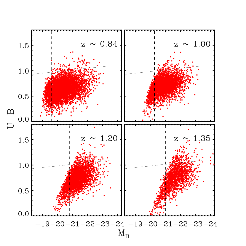
Figure 2.— Rest-frame color-magnitude diagrams. The thin dashed lines show the division between blue galaxies and red galaxies (see Willmer et al. 2006), and the thick dashed lines show the approximate $M_{B}$ completeness limit for our sample.

Unfortunately, we are unable to constrain the faint end of the [O II] LF, especially in the highest redshift bin. Because we do not know the intrinsic number of [O II] emitters within a certain [O II] luminosity bin, we can not calculate the completeness of [O II] luminosity directly, but can only infer that from the completeness of broad-band properties. To analyze the completeness, and in particular to test the significance of the observed turnover (TO) in the LF (vertical dotted lines; Fig. 1), we construct two diagnostic diagrams. In Figure 2 we show the $U-B$ versus $M_{B}$ color-magnitude diagram for our sample. We plot the approximate $B$-band completeness limits for blue galaxies as dashed lines, where the sloping color cut has been defined by Willmer et al. (2006), and the thick vertical dashed line roughly corresponds to where the data and the color cut begin to deviate. In Figure 3 we plot the density distribution of points in the $M_{B}-\log(L_{\mathrm{[OII]}})$ plane in grey scale; the two contours enclose $50\%$ and $80\%$ of the points, respectively. The thin dashed lines in this figure all have a slope of $-3.1~{}\mathrm{mag~{}dex^{-1}}$. This slope is formally consistent with performing a mean ordinary least square fit to the data (Isobe et al. 1990). For our purposes, we note that the line roughly bisects the distribution of points in each panel, i.e., it approximates the median relation between $L_{\mathrm{[OII]}}$ and $M_{B}$. The thick horizontal dashed lines in each panel are equivalent to the thick vertical dashed line plotted in the respective panels in Figure 2, and the vertical dotted lines give the position of the turnover in the respective [O II] LF (Fig. 1). The majority of the galaxies missing from our sample should be along and to the left of the thin dashed line.

Figure 3 demonstrates that, brighter than the turnover, we expect the sample to be complete because the majority of the unobserved galaxies below the $M_{B}$ completeness limit are along and to the left of the thin dashed line. Fainter than the turnover, the sample becomes increasingly incomplete. In the two lowest redshift bins, the turnovers appear to be significant, because fainter than the turnover the difference between the measured LF and the extrapolation of the power law fitted to the bright part of the LF is so significant that it is unlikely to be due to incompleteness. In the two highest redshift bins, however, because the $M_{B}$ completeness limit is very bright, it is possible that the turnovers are artificial, caused by the incompleteness of the survey. In the highest redshift bin, the $M_{B}$ completeness limit is so bright that the slope of the LF may be even steeper than we have derived.

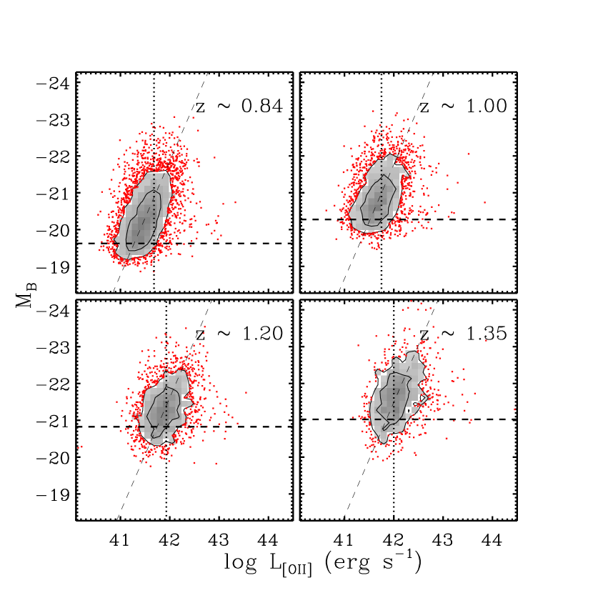
Figure 3.— $M_{B}-\log(L_{\mathrm{[OII]}})$ distribution. The dotted lines are the same as in Figure 1. The thick dashed lines show the $M_{B}$ approximate completeness limit for blue galaxies (see Figure 2). The thin dashed lines have a slope of $-3.1~{}\mathrm{mag~{}dex^{-1}}$, and show the approximate median relation between $M_{B}$ and $\log(L_{\mathrm{[OII]}})$.

To summarize, we are unable to constrain the faint end of the [O II] luminosity function. However, we emphasize that the evolutionary analysis presented in $\S 4$ is unaffected by our inability to constrain the faint-end slope, because we restrict our analysis to the bright part of the [O II] LF where we are statistically complete. In $\S 5$, when integrating the [O II] LF to obtain an estimate of the SFR density, we do make some simplified assumptions regarding the form of the faint end of the LF.

In Figure 4, we compare our results at $z\sim 1.2$ with three other recent coeval measurements of the [O II] LF based on narrow-band observations (Ly07, Takahashi07). Using Subaru/NB816 narrow-band imaging of the $875~{}\mathrm{arcmin}^{2}$ Subaru Deep Field (SDF) by Kashikawa et al. (2004), Ly07 and Takahashi07 identified $894$ and $602$ [O II]-emitting galaxies, respectively. In the $2~{}\mathrm{deg}^{2}$ Cosmic Evolution Survey field (COSMOS; Scoville et al. 2007), Takahashi07 used the same narrow-band filter to identify $5824$ [O II]-emitting galaxies at $z\sim 1.2$ (Taniguchi et al., 2007). Over the range of [O II] luminosity where all the surveys are complete, $10^{42.0}~{}\mathrm{erg~{}s^{-1}}\lesssim L_{\mathrm{[OII]}}\lesssim 10^{42.7}~{}\mathrm{erg~{}s^{-1}}$, we find that our LF from DEEP2 agrees very well with the luminosity functions derived by Ly07 and Takahashi07 in the SDF and COSMOS fields, respectively. It is not clear why the LF of the SDF derived by Takahashi07 is so discrepant with the other surveys, although cosmic variance may play a role. Nevertheless, this comparison shows that: (1) our assumptions regarding the faint-end slope are reasonable; and (2) the bright end of the [O II] LF is clearly a power law, not a Schechter function.

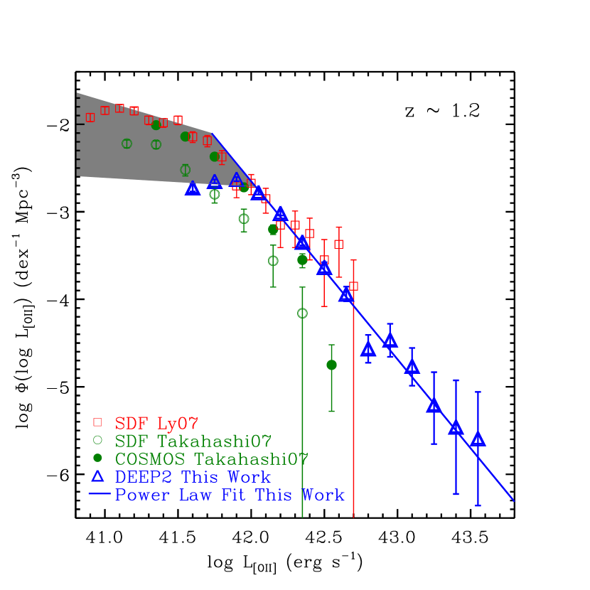
Figure 4.— Comparison of our [O II] luminosity function at $z\sim 1.20$ with other recent measurements from the literature based on narrow-band imaging. The open triangles and the solid line represent our data and best-fitting power law (Fig. 1, lower-left panel). The open squares represent the LF in the Subaru Deep Field (SDF) calculated by Ly et al. (2007) at $z\sim 1.18$. The open and filled circles correspond to observations of galaxies at $z\sim 1.19$ in the SDF and COSMOS fields, respectively (Takahashi et al., 2007). Finally, the shaded region represents our assumption for the faint-end slope when we convert the [O II] LF to SFR density in $\S 5$.

4. The Evolution of the [O II] Luminosity Function

The uncertainty in the faint end of the [O II] LF prevents us from obtaining a reliable estimate of the total [O II] luminosity density. Therefore, we focus instead on the integrated number density, $\phi\equiv\int_{L}^{\infty}\Phi(L)\,dL$, of the strongest [O II]-emitting galaxies. Assuming that the turnover luminosity in the highest redshift bin is $\leq 10^{42}~{}\mathrm{erg~{}s^{-1}}$, we integrate our model of the LF in each redshift bin over $L_{\mathrm{[OII]}}>10^{42}~{}\mathrm{erg~{}s^{-1}}$, and present the results in the top panel of Figure 5 and in Table 2. The horizontal error bars indicate the range of each redshift bin, and the vertical error bars are given by the cosmic variance among the four fields, which dominate the error budget. We find that the total number density of the strongest [O II]-emitting galaxies, i.e., those with $L_{\mathrm{[OII]}}>10^{42}~{}\mathrm{erg~{}s^{-1}}$, declines by a factor of $\gtrsim 2.5$ between $z\sim 1.35$ and $z\sim 0.84$. A linear fit to the four points gives a slope of $\sim 0.9$ dex per unit redshift:

$$\log\left[\phi(L_{\mathrm{[OII]}}>10^{42}~{}\mathrm{erg~{}s^{-1}})\right]=a~{}z-b\mathrm{,}$$ (7)

with $(a,b)$ = $(0.90\pm 0.14,-4.43\pm 0.18)$ and $\phi(L_{\mathrm{[OII]}}>10^{42}~{}\mathrm{erg~{}s^{-1}})$ in $\mathrm{Mpc^{-3}}$. This fit is shown as the dashed line in Figure 5.

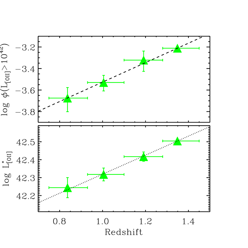
Figure 5.— Evolution of the [O II] luminosity function. (Top) Evolution of the total number density in $\mathrm{Mpc^{-3}}$ of the strongest [O II]-emitting galaxies with $L_{\mathrm{[OII]}}>10^{42}~{}\mathrm{erg~{}s^{-1}}$. The dashed line is the linear fit to the data given by eq. (7). (Bottom) Evolution of the characteristic luminosity, in $\mathrm{erg~{}s^{-1}}$, defined by where the space density of [O II]-emitting galaxies equals $10^{-3.5}~{}\mathrm{dex^{-1}Mpc^{-3}}$. The dotted line is the linear fit to the data given by eq. (8).

The observed decrease in the number density of [O II]-emitting galaxies may be caused by the decline of the overall number density of galaxies in the Universe, or by the evolution of the luminosity function itself. We attempt to constrain the amount of evolution by measuring the luminosity at a fixed space density (see, e.g., Brown et al. 2007). We define a characteristic luminosity, $L_{\mathrm{[OII]}}^{*}$, where the space density equals $10^{-3.5}~{}\mathrm{dex}^{-1}\mathrm{Mpc}^{-3}$, which has the advantage that it is independent of the faint end of the LF. We show $L_{\mathrm{[OII]}}^{*}$ as a function of redshift in the bottom panel of Figure 5, and list the results in Table 2. Once again, the vertical error bars are dominated by cosmic variance. We find that $L_{\mathrm{[OII]}}^{*}$ declines by a factor of $\sim 1.8$ between $z\sim 1.35$ and $z\sim 0.84$. We perform a linear fit to the four points and obtain a slope of $\sim 0.5$ dex per unit redshift:

$$\log L_{\mathrm{[OII]}}^{*}=c~{}z+d\mathrm{,}$$ (8)

with $(c,d)$ = $(0.53\pm 0.07,41.79\pm 0.09)$ and $L_{\mathrm{[OII]}}$ in $\mathrm{erg~{}s^{-1}}$. The resulting fit is shown as the dotted line in Figure 5.

To summarize, we find that the total number density of the strongest [O II]-emitting galaxies has declined by a factor of $\gtrsim 2.5$ between $z\sim 1.35$ and $z\sim 0.84$, when the Universe aged from $4.6$ Gyr to $6.4$ Gyr. This decline may be driven by a decline in the overall number density of galaxies in the Universe, or by a fading of the [O II] LF. Unfortunately, we are unable to establish whether number-density evolution, luminosity evolution, or a combination of both is responsible for the observed evolution. Nevertheless, if we assume that the observed change in the [O II] LF is predominantly due to luminosity evolution, that $L_{\mathrm{[OII]}}$ is proportional to the SFR (see $\S 5$), and that the typical dust attenuation in galaxies at fixed [O II] luminosity does not change significantly over $0.75<z<1.45$, then this result implies that the SFR in galaxies declines by $\sim 25\%$ per Gyr during this epoch. In the next section we integrate the full [O II] LF using some simple assumptions, and compare our results with other estimates of the SFR density at $z\sim 1$.

5. The Evolution of the Star Formation Rate Density

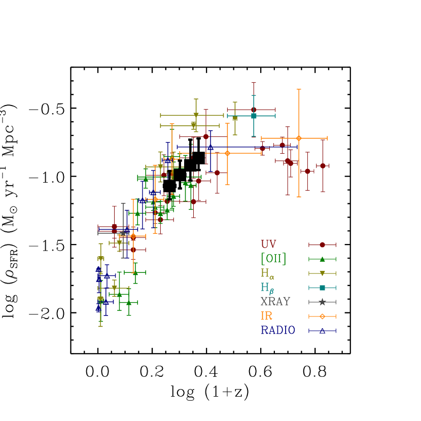
Figure 6.— SFR density, $\rho_{\rm SFR}$, versus redshift based on various multi-wavelength SFR indicators (Hopkins, 2004). Our four estimates of $\rho_{\rm SFR}$ are shown as large filled squares, where the vertical error bars are obtained by allowing the turnover positions and the slope of the faint end of the [O II] luminosity function to vary in a sensible way (see text for details).

Converting the observed [O II] luminosity into a SFR is subject to considerable random and systematic uncertainties, arising from variations in dust attenuation, metallicity, and excitation among star-forming galaxies (Kennicutt, 1992; Jansen et al., 2001; Kewley et al., 2004; Mouhcine et al., 2005; Moustakas et al., 2006). Nevertheless, our measurement of the [O II] luminosity function affords a valuable opportunity to constrain the SFR density of the Universe during an important epoch of cosmic history.

In a recent analysis, Moustakas et al. (2006) showed that dust reddening, as derived using the H$\alpha$/H$\beta$ Balmer decrement, is responsible for the bulk of the scatter in [O II] as a SFR indicator, while variations in metallicity and excitation are second-order effects for most galaxies. Unfortunately, the DEEP2 spectra do not span a sufficiently wide wavelength range to include H$\alpha$, H$\beta$, and other emission-line diagnostics of the metallicity and excitation. Therefore, we use the empirical correlation derived by Moustakas et al. (2006) between the absolute $B$-band magnitude, and the $L_{\mathrm{[OII]}}$/SFR ratio. This calibration statistically accounts for the gross systematic effects of reddening, metallicity, and excitation, all of which correlate with optical luminosity, and has been shown to work reasonably well for star-forming galaxies at $0.7<z<1.4$ (Moustakas et al., 2006; Cooper et al., 2008). Note that an [O II] SFR conversion that is independent of luminosity (e.g., Kennicutt, 1998) would severely underestimate the SFR, because luminous, star-forming galaxies tend to be dustier and more metal-rich (Moustakas et al., 2006).

Another potential concern is that some fraction of the [O II] emission might be arising from an active galactic nucleus (AGN) rather than star formation. Although the AGN-sensitive [N II]/H$\alpha$ ratio (Veilleux & Osterbrock, 1987; Kewley et al., 2001) lies in the near-infrared at $z>0.75$, AGN that contribute significantly to the optical emission-line spectrum also can be identified using [O III] $\lambda 5007$/H$\beta$. In the DEEP2 spectra, [O III]/H$\beta$ is measurable for galaxies at $0.75<z<0.85$, comprising roughly one-third of the sample in our lowest redshift bin. Among these objects, we find $2\%$ ($32/1485$) with $\log\,($[O III]/H$\beta$$)>0.7$, indicative of AGN activity. We can also leverage deep X-ray observations of the EGS to identify AGN (Laird et al., 2009). Among the $2579$ galaxies in this field, we find that $1\%$ ($28/2579$) are also X-ray point sources. These results reveal that powerful AGN constitute a negligible fraction of the sources in our sample. However, even if we have significantly underestimated the fraction of AGN in our sample, detailed studies show that the physical conditions in the narrow-line regions of AGN in the local Universe disfavor [O II] emission, which is one advantage of using [O II] as a SFR tracer (Ho, 2005). Indeed, we will show below that our [O II]-based estimate of the SFR density at $0.84<z<1.35$ agrees remarkably well with other multi-wavelength studies. Therefore, we conclude that AGN contamination is a negligible source of error on our results.

Before integrating the observed [O II] LF to derive the SFR density, $\rho_{\rm SFR}$, we must make some assumptions regarding the form of the faint end of the LF (see $\S 3$). First, we allow the luminosity of the turnover in the LF in each redshift bin to vary over a sensible range of values to account for the uncertainties in our completeness. Specifically, for the two lowest redshift bins, we assume $\log(L_{\mathrm{TO}})$ = $41.68\pm 0.10$ and $41.75\pm 0.10$ $\mathrm{erg~{}s^{-1}}$, respectively, while for the two highest redshift bins, we adopt a fainter lower limit: $\log(L_{\mathrm{TO}})$ = $41.93^{+0.10}_{-0.20}$ and $42.00^{+0.10}_{-0.20}$ $\mathrm{erg~{}s^{-1}}$.

Second, we must assume a form for the [O II] LF fainter than the turnover luminosity. Previous studies (e.g. Gallego et al. 2002; Ly et al. 2007) have assumed that the [O II] LF is a Schechter function, which is a power law at the faint end. However, the faint-end slope, $\alpha_{\mathrm{faint}}$, is usually not well-constrained. Consequently, hereafter we allow $\alpha_{\mathrm{faint}}$ to vary between $-1.1$ and $-1.5$, which brackets the value, $\alpha_{\mathrm{faint}}=-1.3\pm 0.2$, that we measure from the lowest redshift bin in Figure 1. For comparison, Willmer et al. (2006) assumed a faint-end slope of $-1.3$ for the $B$-band LF of blue galaxies at $0.3<z<1.3$.

To summarize, we assume that the [O II] luminosity function is a double power law with slope:

$$\left\{\begin{array}[]{lcc}\alpha_{\mathrm{faint}}=-1.3\pm 0.2&{\rm for}&L_{\mathrm{[OII]}}<L_{\mathrm{TO}}\\ \alpha&{\rm for}&L_{\mathrm{[OII]}}\geq L_{\mathrm{TO}}\end{array}\right.$$

where $\alpha$ is derived from our fit to the bright part of the LF where we are complete. Given these assumptions, we integrate the observed LFs and list the results in Table 2.

Instead of using the $B$-band luminosity of each individual galaxy, we obtain a statistical estimate of $M_{B}$ for each object from $L_{\mathrm{[OII]}}$ using the thin dashed line in Figure 3. We then calculate the appropriate $L_{\mathrm{[OII]}}$/SFR conversion factor by interpolating Table 2 in Moustakas et al. (2006) to derive the SFR.

Figure 5 compares our measurements of $\rho_{\rm SFR}$ at $z\sim 1$ against a large compilation of multi-wavelength measurements from the literature by Hopkins (2004). Our results agree remarkably well with these independent measurements considering the uncertainties in converting $L_{\mathrm{[OII]}}$ into a SFR, and our incompleteness at the faint end of the LF.

6. Conclusions

Because its blue rest-frame wavelength and intrinsic strength allow it to be measured up to $z\sim 1.6$ in the optical, the [O II] $\lambda\lambda 3726,3729$ doublet plays a unique role in the study of galaxy evolution. We have used spectroscopy of $\sim 14,000$ galaxies from the DEEP2 galaxy redshift survey to measure the [O II] luminosity function at $0.75<z<1.45$. Our sample is orders-of-magnitude larger than previous spectroscopic studies, over a considerable larger area spanning four independent fields, allowing us to minimize the systematic effects of cosmic variance. Our principal results are given in Tables 1 and 2, and illustrated in Figures 1 and 5. We found that the bright part of the [O II] LF is well-represented by a power law $dN/dL\propto L^{\alpha}$ with slope $\alpha\sim-3$. However, survey incompleteness prevented us from constraining the faint end of the LF.

We measured the evolution of the [O II] LF using two quantities that only rely on the bright part of the [O II] LF where we are statistically complete. First, we calculated the total number density of galaxies with $L_{\mathrm{[OII]}}>10^{42}~{}\mathrm{erg~{}s^{-1}}$, and found that it has declined by a factor of $\gtrsim 2.5$ between $z\sim 1.35$ and $z\sim 0.84$. Second, we calculated the characteristic luminosity, the luminosity where the space density of [O II]-emitting galaxies equals $10^{-3.5}~{}\mathrm{dex^{-1}Mpc^{-3}}$, and found that it has declined by a factor of $\sim 1.8$ over the same redshift interval. Assuming that the [O II] luminosity is proportional to the SFR, these results imply that the SFR in galaxies declined by $\sim 25\%$ per Gyr during this epoch.

Finally, we used the empirical calibration between $L_{\mathrm{[OII]}}$ and SFR published by Moustakas et al. (2006), and adopted some simple assumptions regarding the faint end of the [O II] LF, to obtain an estimate of the integrated SFR density, $\rho_{\rm SFR}$, in four redshift bins centered around $z\sim 1$. We found that, despite the considerable uncertainties, the evolution we measure is consistent with previous measurements based on a variety of independent, multi-wavelength SFR indicators.

Table 1observed [O II] luminosity function

$\log L_{\mathrm{[OII]}}$	$~{}~{}~{}0.75<z<0.93~{}~{}~{}$				$~{}~{}~{}0.93<z<1.10~{}~{}~{}$				$~{}~{}~{}1.10<z<1.28~{}~{}~{}$				$~{}~{}~{}1.28<z<1.45~{}~{}~{}$
(ergs s${}^{-1})$	$\Phi$	$\sigma_{\mathrm{cv}}$	$N_{gal}$		$\Phi$	$\sigma_{\mathrm{cv}}$	$N_{gal}$		$\Phi$	$\sigma_{\mathrm{cv}}$	$N_{gal}$		$\Phi$	$\sigma_{\mathrm{cv}}$	$N_{gal}$
$41.15$	$49.49^{+3.58}_{-3.34}$	$7.30$	$553$		$\cdots$	$\cdots$	$\cdots$		$\cdots$	$\cdots$	$\cdots$		$\cdots$	$\cdots$	$\cdots$
$41.30$	$60.57^{+3.46}_{-3.27}$	$19.41$	$918$		$20.69^{+2.47}_{-2.22}$	$7.00$	$259$		$\cdots$	$\cdots$	$\cdots$		$\cdots$	$\cdots$	$\cdots$
$41.45$	$56.07^{+2.24}_{-2.15}$	$15.88$	$1095$		$28.25^{+2.03}_{-1.90}$	$2.80$	$524$		$\cdots$	$\cdots$	$\cdots$		$\cdots$	$\cdots$	$\cdots$
$41.60$	$46.93^{+1.94}_{-1.87}$	$7.64$	$1019$		$35.57^{+1.81}_{-1.72}$	$3.95$	$779$		$18.86^{+1.97}_{-1.79}$	$1.57$	$349$		$\cdots$	$\cdots$	$\cdots$
$41.75$	$29.00^{+1.37}_{-1.31}$	$5.82$	$669$		$31.30^{+1.44}_{-1.38}$	$1.32$	$779$		$22.30^{+1.15}_{-1.09}$	$2.03$	$571$		$12.17^{+1.19}_{-1.09}$	$2.22$	$207$
$41.90$	$17.68^{+0.94}_{-0.90}$	$3.68$	$429$		$20.38^{+0.93}_{-0.89}$	$2.64$	$574$		$23.61^{+1.32}_{-1.25}$	$1.53$	$658$		$15.53^{+1.18}_{-1.09}$	$1.74$	$303$
$42.05$	$7.91^{+0.80}_{-0.72}$	$1.57$	$176$		$11.60^{+0.72}_{-0.68}$	$1.30$	$332$		$16.60^{+0.93}_{-0.88}$	$0.44$	$506$		$16.66^{+1.23}_{-1.15}$	$0.94$	$376$
$42.20$	$4.70^{+0.55}_{-0.50}$	$1.63$	$104$		$6.14^{+0.81}_{-0.72}$	$0.46$	$150$		$9.63^{+0.60}_{-0.57}$	$0.96$	$321$		$9.70^{+0.77}_{-0.71}$	$0.53$	$247$
$42.35$	$1.62^{+0.35}_{-0.29}$	$0.55$	$35$		$2.77^{+0.60}_{-0.50}$	$0.98$	$71$		$4.52^{+0.42}_{-0.39}$	$1.16$	$150$		$5.59^{+0.51}_{-0.47}$	$0.97$	$155$
$42.50$	$1.10^{+0.49}_{-0.35}$	$0.44$	$19$		$1.13^{+0.54}_{-0.38}$	$0.34$	$23$		$2.33^{+0.33}_{-0.29}$	$0.56$	$73$		$3.99^{+0.51}_{-0.45}$	$0.38$	$108$
$42.65$	$0.18^{+0.15}_{-0.09}$	$0.11$	$4$		$0.78^{+0.22}_{-0.17}$	$0.32$	$21$		$1.15^{+0.24}_{-0.20}$	$0.33$	$37$		$1.93^{+0.32}_{-0.28}$	$0.48$	$52$
$42.80$	$0.18^{+0.21}_{-0.11}$	$0.24$	$3$		$0.27^{+0.14}_{-0.10}$	$0.18$	$8$		$0.27^{+0.12}_{-0.09}$	$0.11$	$10$		$0.87^{+0.23}_{-0.18}$	$0.28$	$24$
$42.95$	$0.27^{+0.15}_{-0.10}$	$0.12$	$7$		$0.07^{+0.09}_{-0.04}$	$0.06$	$2$		$0.34^{+0.18}_{-0.12}$	$0.21$	$9$		$0.55^{+0.19}_{-0.14}$	$0.18$	$15$
$43.10$	$0.09^{+0.12}_{-0.06}$	$0.09$	$2$		$0.15^{+0.12}_{-0.07}$	$0.08$	$4$		$0.17^{+0.11}_{-0.07}$	$0.10$	$6$		$0.11^{+0.11}_{-0.06}$	$0.12$	$3$
$43.25$	$\cdots$	$\cdots$	$\cdots$		$0.06^{+0.09}_{-0.04}$	$0.08$	$2$		$0.06^{+0.08}_{-0.04}$	$0.06$	$2$		$0.20^{+0.13}_{-0.08}$	$0.13$	$6$
$43.40$	$0.04^{+0.08}_{-0.03}$	$0.08$	$1$		$\cdots$	$\cdots$	$\cdots$		$0.03^{+0.08}_{-0.03}$	$0.05$	$1$		$0.13^{+0.11}_{-0.06}$	$0.08$	$4$
$43.55$	$\cdots$	$\cdots$	$\cdots$		$0.03^{+0.08}_{-0.03}$	$0.06$	$1$		$0.03^{+0.06}_{-0.02}$	$0.04$	$1$		$0.18^{+0.21}_{-0.11}$	$0.24$	$3$
$43.70$	$\cdots$	$\cdots$	$\cdots$		$\cdots$	$\cdots$	$\cdots$		$\cdots$	$\cdots$	$\cdots$		$0.03^{+0.07}_{-0.02}$	$0.07$	$1$
$43.85$	$\cdots$	$\cdots$	$\cdots$		$0.03^{+0.08}_{-0.03}$	$0.05$	$1$		$\cdots$	$\cdots$	$\cdots$		$0.03^{+0.08}_{-0.03}$	$0.04$	$1$

Note. — $\Phi$ is in units of $10^{-4}~{}\mathrm{dex}^{-1}$ Mpc^-3, $\sigma_{\rm cv}$ is the $1\sigma$ uncertainty in $\Phi$ due to cosmic variance, and $N_{gal}$ is the number of galaxies in each bin. For reference, the median redshifts of the sources in each of the four redshift bins are $0.837$, $1.005$, $1.191$, and $1.349$, respectively.

Table 2parameters of the observed [O II]  luminosity functions

Quantity	$0.75<z<0.93$	$0.93<z<1.10$	$1.10<z<1.28$	$1.28<z<1.45$
$z_{\mathrm{median}}$	$0.837$	$1.005$	$1.191$	$1.349$
$N_{\mathrm{gal}}$	$5471$	$3771$	$3018$	$1684$
Age of Universe ($\mathrm{Gyr}$)	$6.46$	$5.73$	$5.06$	$4.59$
$\alpha$	$-3.01\pm 0.07$	$-2.98\pm 0.08$	$-3.03\pm 0.07$	$-2.79\pm 0.12$
$\beta$	$-4.01\pm 0.04$	$-3.86\pm 0.04$	$-3.67\pm 0.03$	$-3.49\pm 0.03$
$\log\Phi(L_{\mathrm{[OII]}}>10^{42}~{}\mathrm{erg~{}s^{-1}})$	$-3.67^{+0.10}_{-0.13}$	$-3.53^{+0.07}_{-0.08}$	$-3.32^{+0.08}_{-0.10}$	$-3.21^{+0.01}_{-0.01}$
$\log$ $L_{\mathrm{[OII]}}^{*}$	$42.24\pm 0.06$	$42.32\pm 0.04$	$42.42\pm 0.03$	$42.50\pm 0.01$
$\log L_{\mathrm{TO}}$	$41.68\pm 0.10$	$41.75\pm 0.10$	$41.93^{+0.10}_{-0.20}$	$42.00^{+0.10}_{-2.00}$
$\log~{}\rho(\mathrm{L_{[OII]}})$	$39.34^{+0.19}_{-0.16}$	$39.40^{+0.19}_{-0.16}$	$39.44^{+0.30}_{-0.17}$	$39.47^{+0.24}_{-0.13}$
$\rho_{\mathrm{S}FR}$	$0.09^{+0.02}_{-0.02}$	$0.10^{+0.03}_{-0.02}$	$0.12^{+0.07}_{-0.03}$	$0.14^{+0.05}_{-0.03}$

References

- Blanton (2006) Blanton, M. R., et al. 2006, ApJ, 648, 268
- Blanton & Roweis (2007) Blanton, M. R., & Roweis, S. 2007, AJ, 133, 734
- Brown et al. (2007) Brown, M. J. J., et al. 2007, ApJ, 654, 858
- Coil et al. (2004) Coil, A. L., et al. 2004, ApJ, 617, 765
- Cooper et al. (2008) Cooper, M. C., et al. 2008, MNRAS, 383, 1058
- Davis et al. (2003) Davis, M., et al. 2003, Proc. SPIE, 4834, 161
- Davis et al. (2007) Davis, M., et al. 2007, ApJ, 660, L1
- Faber et al. (2003) Faber, S. M., et al. 2003, Proc. SPIE, 4841, 1657
- Felten (1976) Felten, J. E. 1976, ApJ, 207, 700
- Gallego et al. (1995) Gallego, J., Zamorano, J., Aragón-Salamanca, A., & Rego, M. 1995, ApJ, 455, L1
- Gallego et al. (2002) Gallego, J., García-Dabó, C. E., Zamorano, J., Aragón-Salamanca, A., & Rego, M. 2002, ApJ, 570, L1
- Gehrels (1986) Gehrels, N. 1986, ApJ, 303, 336
- Glazebrook et al. (1999) Glazebrook, K., Blake, C., Economou, F., Lilly, S., & Colless, M. 1999, MNRAS, 306, 843
- Hammer et al. (1997) Hammer, F., et al. 1997, ApJ, 481, 49
- Hippelein et al. (2003) Hippelein, H., et al. 2003, A&A, 402, 65
- Ho (2005) Ho, L. C. 2005, ApJ, 629, 680
- Hogg et al. (1998) Hogg, D. W., Cohen, J. G., Blandford, R., & Pahre, M. A. 1998, ApJ, 504, 622
- Hogg (1999) Hogg, D. W. 1999, arXiv:astro-ph/9905116
- Hopkins et al. (2000) Hopkins, A. M., Connolly, A. J., & Szalay, A. S. 2000, AJ, 120, 2843
- Hopkins (2004) Hopkins, A. M. 2004, ApJ, 504, 622
- Hopkins & Beacom (2006) Hopkins, A. M., & Beacom, J. F. 2006, ApJ, 651, 142
- Isobe et al. (1990) Isobe, T., Feigelson, E. D., Akritas, M. G., & Babu, G. J. 1990, ApJ, 364, 104
- Jansen et al. (2001) Jansen, R. A., Franx, M., & Fabricant, D. 2001, ApJ, 551, 825
- Kashikawa et al. (2004) Kashikawa, N., et al. 2004, PASJ, 56, 1011
- Kauffmann et al. (2003) Kauffmann, G. et al. 2003, MNRAS, 346, 1055
- Kennicutt (1983) Kennicutt, R. C. 1983, ApJ, 272, 54
- Kennicutt (1992) Kennicutt, R. C. 1992, ApJ, 388, 310
- Kennicutt (1998) Kennicutt, R. C. 1998, ARA&A, 36, 189
- Kennicutt (2008) Kennicutt, R. C. 2008, ApJS, 178, 247
- Kewley et al. (2001) Kewley, L. J., Heisler, C. A., Dopita, M. A., & Lumsden, S. 2001, ApJS, 132, 37
- Kewley et al. (2004) Kewley, L. J., Geller, M. J., & Jansen, R. A. 2004, AJ, 127, 2002
- Laird et al. (2009) Laird, E. S., et al. 2009, ApJS, 180, 102
- Lilly et al. (1996) Lilly, S. J., Le Fevre, O., Hammer, F., & Crampton, D. 1996, ApJ, 460, L1
- Lin et al. (2008) Lin, L., et al. 2008, ApJ, 681, 232
- Ly et al. (2007) Ly, C., et al. 2007, ApJ, 657, 738
- Madau et al. (1996) Madau, P., Ferguson, H. C., Dickinson, M. E., Giavalisco, M., Steidel, C. C., Fruchter, A. 1996, MNRAS, 283, 1388
- Mouhcine et al. (2005) Mouhcine, M., Lewis, I., Jones, B., Lamareille, F., Maddox, S. J., & Contini, T. 2005, MNRAS, 362, 1143
- Moustakas & Kennicutt (2006) Moustakas, J., & Kennicutt, R. C., Jr. 2006, ApJS, 164, 81
- Moustakas et al. (2006) Moustakas, J., Kennicutt, R. C., Jr., & Tremonti, C. A. 2006, ApJ, 642, 775
- Rigopoulou et al. (2005) Rigopoulou, D. 2005, A&A, 440, 61
- Schechter (1976) Schechter, P. 1976, ApJ, 203, 297
- Scoville et al. (2007) Scoville, N., et al. 2007, ApJS, 172, 150
- Takahashi et al. (2007) Takahashi, M., et al. 2007, ApJS, 172, 456
- Taniguchi et al. (2007) Taniguchi, Y., et al. 2007, ApJS, 172, 9
- Teplitz et al. (2003) Teplitz, H. I., Collins, N. R., Gardner, J. P., Hill, R. S., & Rhodes, J. 2003, ApJ, 589, 704
- Tresse et al. (1998) Tresse, L., & Maddox, S. J. 1998, ApJ, 495, 691
- Tresse et al. (2002) Tresse, L., Maddox, S. J., Le Fevre, O., & Cuby, J. -G. 2002, MNRAS, 337, 369
- Veilleux & Osterbrock (1987) Veilleux, S., & Osterbrock, D. E. 1987, ApJS, 63, 295
- Weiner et al. (2007) Weiner, B. J., et al. 2007, ApJ, 660, L39
- Willmer et al. (2006) Willmer, C. N. A., et al. 2006, ApJ, 647, 853
- Yan et al. (1999) Yan, L., McCarthy, P. J., Freudling, W., Teplitz, H. I., Malumuth, E. M., Weymann, R. J., & Malkan, M. a. 1999, ApJ, 519, L47