Three-Dimensional Simulations of Solar and Stellar Dynamos: The Influence of a Tachocline

Abstract

We review recent advances in modeling global-scale convection and dynamo processes with the Anelastic Spherical Harmonic (ASH) code. In particular, we have recently achieved the first global-scale solar convection simulations that exhibit turbulent pumping of magnetic flux into a simulated tachocline and the subsequent organization and amplification of toroidal field structures by rotational shear. The presence of a tachocline not only promotes the generation of mean toroidal flux, but it also enhances and stabilizes the mean poloidal field throughout the convection zone, promoting dipolar structure with less frequent polarity reversals. The magnetic field generated by a convective dynamo with a tachocline and overshoot region is also more helical overall, with a sign reversal in the northern and southern hemispheres. Toroidal tachocline fields exhibit little indication of magnetic buoyancy instabilities but may be undergoing magneto-shear instabilities.

1 Introduction

There is little doubt that turbulent convection in the solar envelope must convert kinetic energy into magnetic energy by means of hydromagnetic dynamo action. However, theoretical arguements and numerical simulations of turbulent dynamos suggest that much of this field must be in a disordered state, dominated by small-scale stochastic fluctuations. The challenge of global solar dynamo theory is to account for the ordered component of the magnetic field, that which gives rise to sunspots, large-scale fields features such as dipolar and quadrupolar moments, and the 22-year activity cycle.

Advances in solar dynamo theory over the past several decades suggest that boundary layers may play a crucial role in generating this ordered magnetic field component. In particular, the solar tachocline located near the base of the convective envelope may be a breeding ground for the manufacture and accumulation of large-scale magnetic flux. There are several reasons for this. (I) Convective expulsion, turbulent pumping, and global meridional circulations continually transport magnetic field into the tachocline region where it can accumulate. (II) Rotational shear amplifies mean toroidal fields through the $\Omega$-effect and suppresses smaller-scale fields by enhancing ohmic diffusion, thus promoting the generation of strong, ordered toroidal flux. (III) The subadiabatic stratification inhibits magnetic buoyancy instabilities, enabling long-term storage of magnetic flux. (IV) The presence of strong, stable large-scale toroidal flux and electrical current structures in the tachocline may provide a magnetic inertia, enhancing and stabilizing the poloidal field component as well. Other processes may also contribute to the generation of ordered magnetic fields and cyclic activity, including the breakup of active regions in the upper boundary layer (the Babcock-Leighton mechanism) and advection of magnetic fields by global meridional circulations (e.g. Charbonneau 2005).

Here we review insight into the nature of global solar and stellar dynamo processes gained from 3D MHD simulations of turbulent convection in rotating spherical shells. We focus on two representative dynamo simulations in a solar context, one in which the computational domain is limited to the convective envelope and one that incorporates convective overshoot into an underlying radiative zone where uniform rotation is imposed, thus creating a mock tachocline. In §2-3 we compare the two simulations and assess how the presence of this tachocline and overshoot region alters the global dynamo. The most apparent difference is the presence of strong, organized toroidal fields in the tachocline region of the latter simulation. In §4 we discuss how such fields may be maintained and address their stability and evolution. In §5 we briefly summarize the implications of these and other stellar dynamo simulations.

2 Simulations and Flow Features

In order to assess the role of a tachocline in global dynamo action we consider two 3D MHD simulations of global solar convection. Both are sustained dynamos that extend over multiple ohmic diffusion time scales. The first is described in detail by Brun, Miesch & Toomre (2004; hereafter BMT04), and is referred to there as Case M3. Here we refer to it as Case A. The second, which we refer to here as Case B, is described further by Browning et al. (2006; hereafter BMBT06; see also Browning et al. 2007). Both simulations are based on the Anelastic Spherical Harmonic (ASH) code with solar values used for the luminosity, rotation rate, and background stratification.

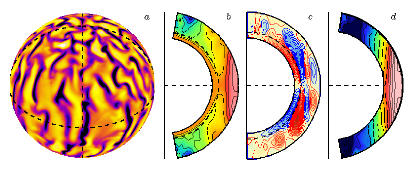
Figure 1: ($a$-$c$) Illustration of convective patterns and mean flows in Case B. ($a$) Orthographic projection of the radial velocity, $v_{r}$ near the middle of the convection zone ($r=0.84R$), with the north pole titled 35^∘ toward the line of sight. Dashed lines indicate the equator and several meridians. Bright tones (yellow/orange in online version) denote upflow and dark tones (blue/black) denote downflow. ($b$) Angular velocity and ($c$) meridional circulation averaged over longitude and time (90 days), the latter represented as streamlines of the mass flux. The dashed line indicates the base of the convection zone. ($d$) The angular velocity in Case A is also shown for comparison. Bright (pink/red) and dark (blue/black) tones denote faster and slower rotation in ($b$) and ($d$), ranging from 350 to 450 nHz. Bright (red) and dark (blue) tones in ($c$) denote clockwise and counter-clockwise circulations respectively, with the flow speed ranging from 2-20 m s^-1.

The principle difference between Cases A and B is the presence of a tachocline in the latter. Whereas the computational domain in Case A stops at the base of the convection zone, $r=0.72R$ where $R$ is the solar radius, Case B incorporates a portion of the subadiabatic radiative interior, extending downward to $r=0.62R$. Both simulations stop short of the solar photosphere, with upper boundaries at (A) $0.97R$ and (B) $0.96R$, in order to avoid complications in the photospheric boundary layer such as granulation, ionization, and the transition to radiative energy transfer which cannot be easily accounted for in our global anelastic modeling framework. The kinematic viscosity, $\nu$, is somewhat higher in Case B, $2\times 10^{12}$ cm² s^-1 in the mid convection zone versus $1.4\times 10^{12}$ cm² s^-1 in Case A, but the magnetic diffusivity $\eta$ is somewhat lower ($P_{m}=4$ in Case A and $P_{m}=8$ in Case B where $P_{m}=\nu/\eta$). Both simulations have comparable spatial resolution. For further details see BMT04 and BMBT06.

A tachocline is imposed in Case B by means of a drag force in the radiative interior that imposes uniform rotation. This is intended to take into account tachocline confinement processes that are not captured by the simulation due to limited spatial resolution and temporal coverage. A thermal forcing is also applied near the base of the convection zone, warming the poles relative to the equator. This is intended to help sustain a strong rotational shear across the tachocline by means of baroclinic torques that partially offset the sub-grid-scale diffusion and that compensate for the extent of the overshoot region which is wider than in the Sun due to computational limitations. We emphasize that the rotational shear in the convective envelope is still maintained by the convective Reynolds stress; the mechanical and thermal forcing merely promotes a sharp tachocline. Such an approach cannot provide much insight into tachocline confinement processes but it can be used to investigate the influence of a tachocline on global dynamo action, which is our motivation. For further discussion see BMBT06.

The convective structure in Cases A and B is similar, dominated at low latitudes in the mid convection zone by columnar convection cells aligned with the rotation axis (Fig. 1$a$), as in comparable non-magnetic simulations (reviewed by Miesch & Toomre 2009). Near the surface both exhibit an interconnected network of downflow lanes laced by vertical magnetic flux (BMT04).

The differential rotation profile in both cases is roughly solar-like (Fig. 1$b$, $d$), with a monotonic decrease in angular velocity $\Omega$ with latitude. However, both exhibit more cylindrical alignment than the solar rotation profile as revealed by helioseismology. Furthermore, the angular velocity contrast $\Delta\Omega$ between equator and pole is much weaker in Case B (about 13% compared to 36% in Case A). This is typical of penetrative convection simulations and may arise in part from our artificially wide overshoot region (Miesch 2007a) and in part from Lorentz forces associated with stronger mean fields (§3). Despite the weaker $\Delta\Omega$, Case B possesses a tachocline; substantial radial shear near the base of the convection zone maintained by our mechanical and thermal forcing.

The most prominent feature of the mean meridional circulation in Case B is an equatorward flow at the base of the convection zone with an amplitude of about 8 m s^-1 (Fig. 1$c$). This may in part be attributed to the thermal forcing but other simulations without such forcing also exhibit equatorward circulation near the base of the convection zone, albeit somewhat weaker (several m s^-1; see Miesch et al. 2000). This has important implications for flux-transport dynamo models as we address in §4. The circulation profile in the bulk of the convection zone is multi-celled, as in Case A (BMT04).

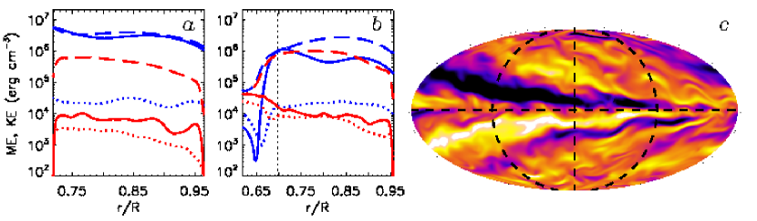
Figure 2: Magentic (black; red in online version) and kinetic (grey; blue) energy density in ($a$) Case A and ($b$) Case B, averaged over horizontal surfaces and over time (4 days). Solid lines denote the energy in the mean toroidal field and the differential rotation, dotted lines that in the mean poloidal field and the meridional circulation, and dashed lines that in the non-axisymmetric field and flow components. The vertical dotted line in ($b$) denotes the base of the convection zone. ($c$) Molleweide projection of the longitudinal field component $B_{\phi}$ in the tachocline of Case B ($r=0.67R$) at a time when $m=1$ structure is particularly evident. Bright and dark tones denote eastward and westward fields respectively.

3 Mean and Fluctuating Fields

As discussed in §1, turbulent flows beget turbulent fields. In both Cases A and B, dynamo action produces strong fluctuating (non-axisymmetric) fields that account for 95-98% of the total magnetic energy in the convection zone (Fig. 2$a$, $b$). Both mean and fluctuating field components are somewhat stronger in Case B, due in part to the lower magnetic diffusivity (§2). More remarkably, the magnetic energy in the mean toroidal field of Case B rises steadily toward the base of the convection zone, peaking in the tachocline where it reaches equipartition with the fluctuating field components and also with the fluctuating kinetic energy. Note that the drop in the differential rotation kinetic energy below $r=0.69R$ is due primarily to the mechanical forcing (§2).

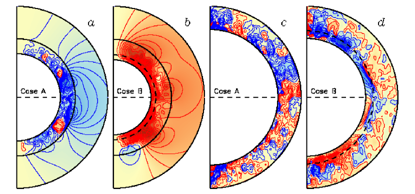
Figure 3: Mean ($a$, $b$) poloidal magnetic fields and ($c$, $d$) toroidal magnetic fields in ($a$, $c$) Case A and ($b$, $d$) Case B, averaged over longitude and time (90 days). White (red in online version) tones denote a clockwise poloidal field orientation and eastward toroidal field whereas black (blue) tones denote the opposite. Saturation levels for the poloidal and toroidal color tables are $\pm$20G and $\pm$2000G respectively. Poloidal fields in ($a$, $b$) include a potential-field extrapolation out to $1.5R$ and the base of the convection zone is indicated by a dashed line in ($b$, $d$).

The structure of the tachocline field in Case B is dominated by strong (2-5 kG) toroidal bands or extended magnetic layers that are roughly antisymmetric about the equator. These toroidal bands are generally axisymmetric as illustrated in Figure 3$d$ but they occasionally exhibit a pronounced $m=1$ component as demonstrated in Figure 2$c$, where $m$ is the longitudinal wavenumber. This $m=1$ behavior may be indicative of magneto-shear instabilities as we discuss in §4. The toroidal bands are remarkably persistent, remaining intact for thousands of days, punctuated sporadically by brief intervals ($<$ 200 days) of roughly symmetric parity about the equator after which the antisymmetric parity is re-established with the same polarity as before (BMBT06, Browning et al. 2007). The simulation has spanned over two decades and has not yet undergone a sustained polarity reversal of the mean toroidal field in the tachocline.

In contrast to the strong, persistent bands in the tachocline, the mean toroidal field in the convection zone of both cases A and B is relatively weak ($\sim$ 1 kG), disordered, and transient (Fig. 3$c$, $d$). This lends support to the arguments put forth in §1 on why the tachocline might be a prime place to generate large-scale magnetic flux. The mean poloidal field in Case B (Fig. 3$b$) also appears stronger and more ordered than in Case A (Fig. 3$a$), with a more prominent dipole moment. This is demonstrated further in Figure 4 which shows the dipole and quadropole moment in each case over thousands of days of evolution.

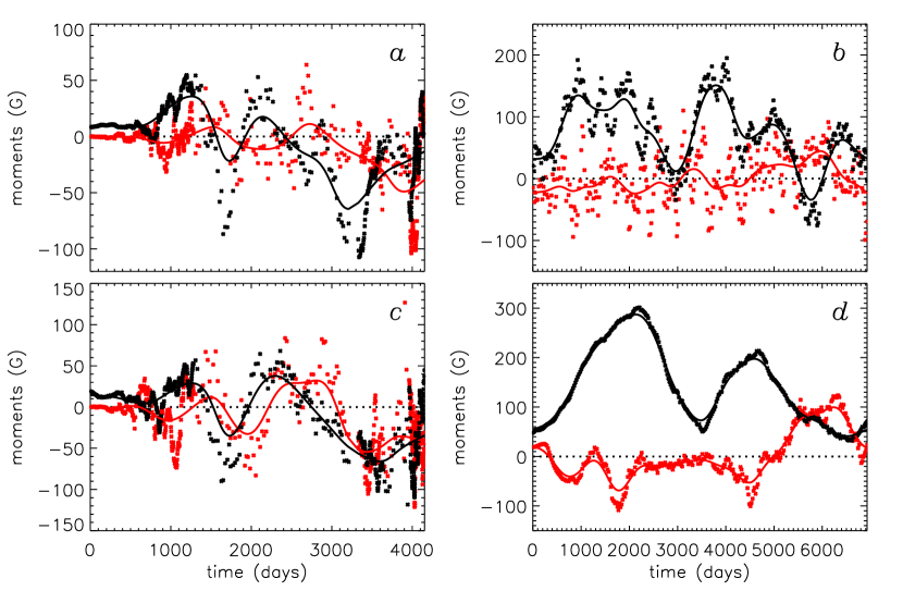
Figure 4: Time evolution of the dipole (black) and quadrupole (grey; red in online version) moments in ($a$, $c$) Case A and ($b$, $d$) Case B. The top row corresponds to the outer boundary in each case ($a$) $0.97R$ and ($b$) $0.96R$ whereas the bottom row corresponds to the base of the convection zone in Case A ($c$) $0.72R$ and to the underlying tachocline in Case B ($d$) $0.67R$. Points denote instantaneous snapshots and lines denote running six-month averages.

In Case A, the dipole and quadrupole moments are comparable in amplitude and erratically reverse sign on a time scale of roughly 500 days. By contrast, the dipole moment in Case B is stronger both in absolute magnitude and relative to the quadrupole component, although this is less so toward the end of the interval shown in Figure 4. The dipole moment is also more stable in Case B, maintaining the same sign through most of the simulation apart from a brief reversal near the top of the shell at $t\sim$ 6000 days. As with any numerical simulation, however, these conclusions are based on a limited time interval. Figure 4$d$ in particular suggests that the dipole moment may be waning over the course of several decades. Further time evolution is necessary to clarify any potential long-term trends, including the possiblity of systematic polarity reversals.

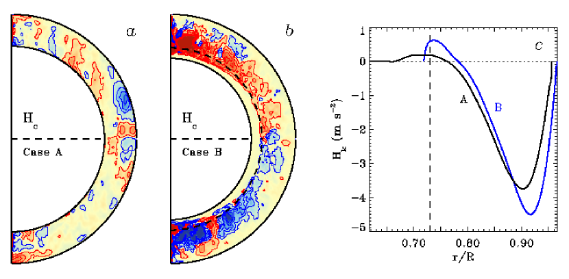
Figure 5: The fluctuating current helicity $\mbox{\boldmath$J$}^{\prime}\mbox{\boldmath$\cdot$}\mbox{\boldmath$B$}^{\prime}$ is shown for ($a$) Case A and ($b$) Case B averaged over longitude and over the same 90-day time interval as in Figures 1 and 3. White and black (red and blue in online version) denote positive and negative values and the color table saturates at $\pm 2\times 10^{7}$ statamp cm^-2 G. ($c$) Kinetic helicity in Case A (black line) and Case B (grey; blue), averaged over the northern hemisphere and time (4 days). Dashed lines in ($b$) and ($c$) denote the base of the convection zone in Case B.

Another remarkable feature of the magnetic field in Case B is illustrated in Figure 5$b$; it is helical. Shown is the current helicity in the fluctuating field component, $H_{c}^{\prime}=\mbox{\boldmath$J$}^{\prime}\mbox{\boldmath$\cdot$}\mbox{\boldmath$B$}^{\prime}$, where $\mbox{\boldmath$J$}=(c/4\pi)\mbox{\boldmath$\nabla\times$}\mbox{\boldmath$B$}$ is the current density and primes indicate that the longitudinal mean has been subtracted out. Although the magnetic helicity $H_{m}=\mbox{\boldmath$A$}\mbox{\boldmath$\cdot$}\mbox{\boldmath$B$}$ is of greater theoretical interest (where $A$ is the vector potential, defined such that $\mbox{\boldmath$B$}=\mbox{\boldmath$\nabla\times$}\mbox{\boldmath$A$}$), $H_{c}$ has the advantage that it is guauge invariant and is more readily observable. Both $H_{c}$ and $H_{m}$ quantify the degree to which the magnetic field topology is twisted and is not reflectionally symmetric.

Magnetic helicity has profound implications for large-scale dynamo action. The turbulent $\alpha$-effect, whereby large-scale fields are generated by small-scale velocity fields, is intimately tied to the upscale spectral transfer of magnetic helicity. If the transfer is local, this is referred to as an inverse cascade. However, the ensuing buildup of small-scale helicity can suppress the inverse cascade if it is not dissipated or removed through the boundaries. This suppression can be so dramatic that it has been referred to as catastrophic $\alpha$-quenching and if it occurs, it would imply that the turbulent $\alpha$-effect cannot account for the mean fields observed in the Sun and other stars. For further discussion see Brandenburg & Subramanian (2005) and Miesch & Toomre (2009).

The helical nature of the fluctuating magnetic field in Case B (Fig. 5$b$) suggests that the presence of a tachocline and overshoot region may mitigate catastrophic $\alpha$ quenching. The convection may be shunting small-scale helicity into the stable zone where it is stored or dissipated, thus promoting helicity generation, and possibly self-organization processes associated with upscale helicity transfer, in the convection zone. By contrast, the fluctuating field in Case A (Fig. 5$a$) is not particularly helical and does not exhibit the asymmetry about the equatorial plane evident in Case B.

The sign of the current helicity in Case B is positive in the north and negative in the south, which is opposite to that inferred from photospheric and coronal measurements (e.g. Pevtsov & Balasubramaniam 2003). However, such measurements are concerned with field structures such as active regions that are associated with the large-scale field component. If such fields are generated through an upscale transfer of magnetic helicity, one would expect that the sense of the helicity should be opposite to that in the fluctuating component. Indeed, the negative $B_{\phi}$ apparent in the northern hemisphere in Fig. 3$d$ coupled with the positive dipole moment apparent in Fig. 3$d$ implies a negative current helicity for the mean field component. Thus, the sign of the current helicity in Case B may be consistent with solar observations.

There are many caveats to this simplified picture, including the poorly understood details of how helicial flux tubes form in the tachocline and emerge. Nevertheless, it is clear that the dynamical aspects of magnetic helicity offer a fertile ground for further insight into the subtleties of global solar and stellar dynamos, particularly with regard to influence of a tachocline.

In contrast to $H_{c}^{\prime}$, the kinetic helicity, $H_{k}=\mbox{\boldmath$\omega$}\mbox{\boldmath$\cdot$}\mbox{\boldmath$v$}$ where $v$ and $\omega$ are the fluid velocity and vorticity, is similar in Cases A and B (Fig. 5$c$). The $H_{k}$ profile in both cases is antisymmetric about the equator, with a negative sign in the northern hemisphere through most of the convection zone. Near the base of the convection zone the sign of $H_{k}$ reverses due largely to the influence of the Coriolis force on diverging downflows. Kinetic helicity profiles such as this are a well known feature of rotating compressible convection (e.g. Gilman 1983; Miesch et al. 2000).

4 Maintenance and Evolution of Tachocline Fields

According to our current understanding of the solar dynamo, we may expect that toroidal fields generated in the tachocline by the $\Omega$-effect should migrate equatorward, intermittently spawning flux tubes as they go which then emerge through the photosphere as active regions. In this section we briefly address how our simulations relate to this prevailing dynamo paradigm.

To this end, we must first understand how the toroidal fields in the tachocline of Case B are established and maintained. A detailed analysis will await a future paper but here we can confirm that the principle source term in generating mean toroidal flux in the tachocline is indeed the $\Omega$-effect arising from radial angular velocity shear $\partial\Omega/\partial r$, as might be expected based on the prevailing paradigm. The latitudinal shear $\partial\Omega/\partial\theta$ also contributes, as does the radial component of the turbulent emf: $E_{r}^{\prime}=v_{\theta}^{\prime}B_{\phi}^{\prime}-v_{\phi}^{\prime}B_{\theta}^{\prime}$.

These generation terms work to offset radial diffusion and the latitudinal advection of toroidal flux by the meridional circulation which both act to erode the tachocline field (latitudinal diffusion is negligible). The latitudinal component of the turbulent emf, $E_{\theta}^{\prime}=v_{\phi}^{\prime}B_{r}^{\prime}-v_{r}^{\prime}B_{\phi}^{\prime}$. also acts as a sink term on average, at least over the 6930-day time interval shown in Fig. 4$b$, $d$. This is somewhat surprising since turbulent pumping of toroidal flux, if it occurs, would be reflected in the $E_{\theta}^{\prime}$ term. Thus, turbulent pumping acts to erode the tachocline field in Case B rather than maintain it. Although this may be contrary to theoretical expectations, it is still consistent with the concept of turbulent pumping since the mean toroidal flux in the convection zone of Case B is opposite in sign (albeit weaker in magnitude) relative to the tachocline field.

Conventional wisdom suggests that as toroidal flux is amplified by rotational shear in the tachocline it will eventually become susceptible to magnetic buoyancy instabilies, forming isolated flux tubes which then rise toward the solar surface. Although some strong, transient toroidal ribbons in Case B do exhibit a slight density deficit which may induce them to rise, the persisent magnetic layer evident in Figure 3$d$ appears to be largely stable. The proximate reason for this is because the layer does not exhibit any significant density evacuation relative to its surroundings but the ultimate explanation is still under investigation. It may be that our subgrid-scale diffusion and our artificially wide overshoot region limits the radial magnetic field gradients that can be achieved. In any case, it is clear that turbulent flows and fields in Case B contribute to the mechanical equilibrium of the magnetic layer and furthermore, the layer is not an isolated magnetic surface; rather, it has field line connectivity to the entire convection zone. Thus, conditions here are far from the idealized equilibrium states typically considered in investigations of magnetic buoyancy instabilities.

Toroidal magnetic fields in the tachocline are also susceptible to another type of instability fed by latitudinal shear, as described by Gilman & Fox (1997). Although higher wavenumber modes may also occur, the most vigorous and robust mode for broad toroidal field profiles (antisymmetric about the equatorial plane) is the $m=1$ clam-shell instability whereby toroidal loops tip out of phase, reconnecting across the equator at one meridian and spreading poleward at the antipode. If the rotational shear is maintained and if the poloidal field is continually replenished, such clam-shell instabilities can occur indefinitely (Miesch 2007b).

The presence of sustained clam-shell instabilities in Case B is suggested by the prominent $m=1$ structure in snapshots such as that shown in Fig. 2$c$. If such instabilites are indeed occurring, one would expect to see a quasi-periodic energy exchange between the $m=0$ and the $m=1$ components of the toroidal field (Miesch 2007b). We will address this in a future paper.

In mean-field dynamo models, the equatorward propagation of toroidal flux implied by the solar butterfly diagram is usually attributed to one of two mechanisms (that are not mutually exclusive). The first is advection by an equatorward meridional circulation near the base of the convection zone and the second is the propagation of a dynamo wave induced by rotational shear and turbulent field generation (the $\alpha$-effect). In the latter case, equatorward propagation is achieved if the product $H_{k}\partial\Omega/\partial r>0$ in the northern hemisphere (e.g. Charbonneau 2005).

Both of these propagation mechanisms could in principle be occurring in Case B. At mid and low latitudes near the base of the convection zone there is a strong equatorward meridional circulation (Fig. 1$c$) and $H_{k}$ and $\partial\Omega/\partial r$ are both positive in the northern hemisphere (Figs. 1$b$, 5$c$). However, the amplitude of the circulation and the kinetic helicity peak above the principle toroidal flux concentration. Perhaps not surprisingly, then, there is little indication for any latitudinal propagation of the tacholine field in Case B.

5 Conclusion

Although 3D MHD dynamo simulations cannot capture all processes of relevance to the global solar dynamo, they can provide crucial insight into key ingredients. In particular, understanding the subtle interaction between turbulent field generation in the convection zone and the generation of toroidal flux by rotational shear in the tachocline stands to benefit greatly from high-resolution MHD simulations of penetrative convection. By providing a reservoir for expelling, amplifying and storing magnetic flux, the tachocline influences the global behavior of the dynamo, promoting strong, stable mean fields and helical magnetic topologies throughout the convection zone.

Throughout this brief paper our emphasis has been on the Sun but stellar dynamo simulations have also produced substaintial insights in recent years. Highlights include the generation of strong toroidal flux structures in rapidly-rotating solar-like stars (Brown et al. 2007), enhancement of core dynamo action in A stars by fossil envelope fields (Featherstone et al. 2007), quenching of $\Delta\Omega$ by the Lorentz force in the deep convective shells of A and M stars (Brun, Browning & Toomre 2005; Browning 2008), and the saturation of $\Delta\Omega$ and mean field strengths at high $\Omega$ (Christensen & Aubert 2006). The latter was done in planetary context but may also have important implications for stars (see Miesch & Toomre 2009).

We thank Nicholas Featherstone, Kyle Augustson and Nicholas Nelson for numerous discussions on all aspects of MHD dynamo simulations and Keith MacGregor for helpful comments on the manuscript. The work presented here was supported by NASA through the Heliophysics Theory Program grant NNG05G124G. The simulations were carried out with NSF PACI support of PSC, SDSC, NCSA, NASA support of Project Columbia, and through the CEA resource of CCRT and CNRS-IDRIS in France.

References

- [Brandenburg & Subramanian] Brandenberg, A. & Subramanian, K. 2005, Astrophysical Magnetic Fields and Nonlinear Dynamo Theory, Phys. Rep., 417, 1-209.
- [Brown et al. 2007] Brown, B.P., Browning, M.K, Brun, A.S., Miesch, M.S., Nelson, N.J & Toomre, J. 2007, Strong Dynamo Action in Rapidly Rotating Suns, in “Unsolved Problems in Stellar Physics; A Conference in Honor of Douglas Gough”, ed. R.J. Stancliffe, G. Houdek, R.G. Martin & C.A. Tout (AIP: Melville, NY), AIP Conf. Proc. vol. 948, 271-278.
- [Browning et al. 2006] Browning, M.K, Miesch, M.S., Brun, A.S. & Toomre, J. 2006, Dynamo Action in the Solar Convection Zone and Tachocline: Pumping and Organization of Toroidal Fields, ApJ, 648, L157-L160 (BMBT06).
- [Browning et al. 2007] Browning, M.K, Brun, A.S. Miesch, M.S. & Toomre, J. 2007, Dynamo Action in Simulations of Penetrative Solar Convection with an Imposed Tachocline, Astron. Nachr., 328, 1100-1103.
- [Browning 2008] Browning, M.K. 2008, Simulations of Dynamo Action in Fully Convective Stars, ApJ, 676, 1262-1280.
- [Brun, Browning & Toomre 2005] Brun, A.S., Browning, M.K. & Toomre, J. 2004, Simulations of Core Convection in Rotating A-Type Stars: Magnetic Dynamo Action, ApJ, 629, 461-481.
- [Brun, Miesch & Toomre 2004] Brun, A.S., Miesch, M.S. & Toomre, J. 2004, Global-Scale Turbulent Convection and Magnetic Dynamo Action in The Solar Envelope, ApJ, 614, 1073-1098 (BMT04).
- [Christensen & Aubert 2006] Christensen, U. & Aubert, J. 2006, Scaling Properties of Convection-Driven Dynamos in Rotating Spherical Shells and Applications to Planetary Magnetic Fields, Geophys. J. Int., 166, 97-114.
- [Charbonneau 2005] Charbonneau, P. 2005, Dynamo Models of the Solar Cycle, Living Rev. Sol. Phys., 2, http://www.livingreviews.org/lrsp-2005-2.
- [Gilman 1983] Gilman, P.A. 1983, Dynamically Consistent Nonlinear Dynamos Driven by Convection in a Rotating Spherical Shell II. Dynamos with Cycles and Strong Feedbacks, ApJ Sup. Ser., 53, 243-268.
- [Gilman & Fox 1997] Gilman, P.A. & Fox, P.A. 1997, Joint Instability of Latitudinal Differential Rotation and Toroidal Magnetic Fields Below the Solar Convection Zone, ApJ, 484, 439-454.
- [Featherstone et al. 2007] Featherstone, N.A., Browning, M.K., Brun, A.S. & Toomre, J. 2007, Dynamo Action in the Presence of an Imposed Magnetic Field, Astron. Nachr., 328, 1126-1130.
- [Miesch 2007a] Miesch, M.S. 2007, Turbulence in the Tachocline, in “The Solar Tachocline”, ed. D.W. Hughes, R. Rosner & N.O. Weiss (Cambridge Univ. Press: Cambridge), Ch. 5, 109-128.
- [Miesch 2007b] Miesch, M.S. 2007, Sustained Magneto-Shear Instabilities in the Solar Tachocline, ApJ, 658, L131-L134
- [Miesch et al. 2000] Miesch, M.S., Elliott, J.R., Toomre, J., Clune, T.C., Glatzmaier, G.A. & Gilman, P.A. 2000, Three-Dimensional Spherical Simulations of Solar Convection: Differential Rotation and Pattern Evolution Achieved with Laminar and Turbulent States, ApJ, 532, 593-615.
- [Miesch & Toomre 2009] Miesch, M.S. & Toomre, J. 2009, Turbulence, Magnetism, and Shear in Stellar Interiors, Ann. Rev. Fluid Mech., in press, advance copy available at http://annualreviews.org.
- [Pevtsov & Balasubramaniam 2003] Pevtsov, A.A. & Balasubramaniam, K.S. 2003, Helicity Patterns on the Sun, Adv. Space Res., 32, 1867-1874.