Universality in Oscillating Flows

Abstract

We show that oscillating flow of a simple fluid in both the Newtonian and the non-Newtonian regime can be described by a universal function of a single dimensionless scaling parameter $\omega\tau$, where $\omega$ is the oscillation (angular) frequency and $\tau$ is the fluid relaxation-time; geometry and linear dimension bear no effect on the flow. Experimental energy dissipation data of mechanical resonators in a rarefied gas follow this universality closely in a broad linear dimension ($10^{-6}$ m$<L<10^{-2}$ m) and frequency ($10^{5}$ Hz $<\omega/2\pi<10^{8}$ Hz) range. Our results suggest a deep connection between flows of simple and complex fluids.

The law of similarity Reynolds (1883); Landau and Lifshitz (1959) is the most basic consequence of the Navier-Stokes equations of fluid dynamics: two geometrically similar flows with different velocities and viscosities but equal Reynolds numbers can be made identical by rescaling the measurement units. Similarity turns into universality Tanaka (1996) if additional characteristics of the flow – such as the constitutive stress-strain relations, the flow geometry, and other dynamical aspects – can all be incorporated into the scaling. For steady flows past solid bodies, for example, the law of similarity can be formulated Landau and Lifshitz (1959) in terms of the velocity field u:

$$\textit{{u}}=\textit{{U}}f(\frac{\textit{{r}}}{L},{\mathop{\rm Re}}).$$ (1)

Here, U is a characteristic velocity of the flow, r represents the position vector, $L$ is a dynamically relevant linear dimension, and ${\mathop{\rm Re}\nolimits}=UL/\nu$ is the Reynolds number with kinematic viscosity $\nu$. The dimensionless scaling function $f$, which reflects subtle features of the flow, is found from the Navier-Stokes equations. Defining the mean free-path and relaxation time as $\lambda$ and $\tau$, respectively, one can express $\nu$ in terms of these microscopic parameters as $\nu\approx\lambda^{2}/\tau\approx\lambda c_{s}$, where $c_{s}$ is speed of sound.

The equations of fluid dynamics can be formulated in the most general form as

$$\frac{\partial u_{i}}{\partial t}+(\textit{{u}}\cdot\nabla){\rm{}}u_{i}=\nabla_{j}\sigma_{ij},$$ (2)

with $i,j=x,y,z$. The stress tensor $\sigma_{ij}$ can be expanded in powers of the Knudsen number $({\rm{Kn}}=\lambda/L)$ and the Weissenberg number $({\rm{Wi}}=\tau/T)$ Landau and Lifshitz (1981); Chen et al. (2004); Cercignani (1975): $\sigma_{ij}=\sigma_{ij}^{(1)}+\sigma_{ij}^{(2)}+...$. Newtonian fluid dynamics, where $\sigma_{ij}=\frac{\mu}{2}(\frac{{\partial u_{i}}}{{\partial x_{j}}}+\frac{{\partial u_{j}}}{{\partial x_{i}}})$ with $\mu=\rho\nu$, corresponds to the first term of the expansion. To see this, simply consider a steady flow past a bluff body of linear dimension $L$: $\frac{\sigma}{{\rho U^{2}}}\approx\frac{\lambda}{L}\frac{{c_{s}}}{U}\approx\frac{\rm{Kn}}{\rm{Ma}}$ given that the velocity gradient $\sim\frac{U}{L}$; here, ${\rm{Ma}}=U/c_{s}$ is the Mach number. Thus, the Newtonian approximation is only valid when $\rm{Kn}\ll 1$. With $\lambda\approx c_{s}\tau$, it is easy to see that $\rm{Kn}=\frac{\lambda}{\textit{L}}\approx\frac{{\textit{c}_{\textit{s}}}}{\textit{U}}\frac{\tau}{\textit{T}}\approx\frac{\rm{{Wi}}}{\rm{Ma}}$ and $\frac{\sigma}{{\rho U^{2}}}\approx\frac{{\rm{Wi}}}{{\rm{Ma^{2}}}}$. Consequently, $\rm{Kn}\ll 1$ and $\rm{Wi}\ll 1$ correspond to the same physical limit for fixed $\rm{Ma}$. This statement can also be extended to an unsteady flow past a bluff body, where the shed vortices may be thought to introduce independent time ($\rm{Wi}$) and length scales ($\rm{Kn}$). Yet, the characteristic oscillation frequency for vortex shedding is given by $\Omega=\frac{{2\pi U\rm{St}}}{L}$, where ${\rm{St}}=\frac{L}{{UT}}$ is the Strouhal number. It is well-known that ${\rm{0}}{\rm{.1}}\leq{\rm{St}}\leq{\rm{1}}$ over a wide range of $\rm{Re}$ depending on geometry. Thus, $\Omega\tau=\frac{{2\pi\tau}}{T}\sim\frac{\lambda}{L}\frac{U}{{c_{s}}}$, and $\rm{Wi}$ and $\rm{Kn}$ are linked. It is then straightforward to conclude that Newtonian fluid dynamics and emerging similarity relations, e.g. Eq. (1), should be valid for slowly-varying large-scale flows: $\rm{Kn}\ll 1$ and $\rm{Wi}\ll 1$.

Recent advances in micro- Squires and Quake (2005) and nanotechnology Karabacak et al. (2007); Verbridge et al. (2008), biofluid mechanics Stroock et al. (2002), rheology Bird et al. (1987), and so on have resulted in flows at unusual time ($\rm{Wi}\geq 1$) and length ($\rm{Kn}\geq 1$) scales, where Newtonian approximation breaks down. Many interesting phenomena, such as elastic turbulence Groisman and Steinberg (2000), structural relaxation of soft matter Wyss et al. (2007) and enhanced heat transfer in nanoparticle-seeded fluids Wang et al. (1999), have been observed in this range of parameters. Thus, a universal description of Newtonian and non-Newtonian flow regimes is of great importance for both fundamental physics and engineering.

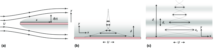
Figure 1: (color online). Flow geometries and dynamical parameters. (a) Laminar steady flow over a semi-infinite flat plate with a viscous boundary layer of thickness $\delta(x)$ and a free stream velocity $U$. (b) Unsteady flow generated by an infinite plate oscillating at (angular) frequency $\omega$ with peak velocity $U$ in the Newtonian limit ($\omega\tau\ll 1$). (c) The same problem in the non-Newtonian limit ($\omega\tau\geq 1$). A wavelength $\delta_{+}$ and a penetration depth $\delta_{-}$ emerge instead of the viscous boundary layer thickness $\delta$.

The similarity law given in Eq. (1) is valid in the Newtonian regime only. For this regime, since both $\rm{Wi}$ and $\rm{Kn}$ are small, $\rm{Re}$ is the only relevant dimensionless parameter. In the non-Newtonian regime, the situation is different. For a similarity law valid in both Newtonian and non-Newtonian regimes, the scaling relation in Eq. (1) could be modified as

$$\textit{{u}}=\textit{{U}}f(\frac{\textit{{r}}}{L},\frac{\textit{{r}}}{\delta},\frac{\lambda}{L},\frac{\lambda}{\delta},\frac{\tau}{T},{\mathop{\rm Re}\nolimits},{\rm{St}}).$$ (3)

This is a prescribed relation including all relevant dimensionless parameters. In addition to the above-mentioned parameters, a dynamic length scale $\delta$ (to be clarified below) may enter the scaling function $f$. The final form of the scaling relation is determined by the physical nature of the flow. In order to assess the relative importance of various dimensionless parameters and reduce the scaling relation in Eq. (3), we investigate the second order correction to the stress tensor derived from the Boltzmann equation Landau and Lifshitz (1981); Chen et al. (2004); Cercignani (1975):

$$\sigma_{ij}^{(2)}\approx\rho\lambda^{2}\frac{{\partial u_{i}}}{{\partial x_{\alpha}}}\frac{{\partial u_{j}}}{{\partial x_{\alpha}}}.$$ (4)

Considering first the shed vortices behind a body, we readily estimate that $\sigma^{(2)}\approx\rho\lambda^{2}U^{2}/L^{2}$. Thus, $\sigma^{(1)}+\sigma^{(2)}\approx\rho\nu\frac{U}{L}+\rho\lambda^{2}\frac{{U^{2}}}{{L^{2}}}\approx\rho\nu\frac{U}{L}(1+\frac{U}{{c_{s}}}\frac{\lambda}{L})\approx\rho\nu\frac{U}{L}(1+\frac{\tau}{T})$. In this simple case, $\sigma$ appears as an expansion in powers of $\rm{Kn}$ or, equivalently, $\rm{Wi}$.

In another classic problem – laminar steady flow over a semi-infinite flat plate illustrated in Fig. 1(a) – the relationship between $\rm{Kn}$ and $\rm{Wi}$ can still be stated, albeit with important differences from above. The key dynamic feature of this flow is the viscosity-dominated boundary layer of thickness $\delta=\sqrt{\frac{{x\nu}}{U}}$. Here, $U$ is the free-stream velocity outside the boundary layer. The Newtonian approximation results in $\sigma_{xy}^{(1)}=\rho\nu\frac{{\partial u_{x}}}{{\partial y}}\approx\rho c_{s}\lambda\frac{U}{\delta}$. With the symmetries in the problem, the contributions to the stress tensor of the kind given in Eq. (4) disappear, resulting in a second order correction Landau and Lifshitz (1981) $\sigma_{xy}^{(2)}=\rho\lambda^{2}\frac{{\partial u_{x}}}{{\partial y}}{\rm{}}(\nabla\cdot\textit{{u}})\approx\rho\lambda^{2}\frac{{U^{2}}}{{x\delta}}$. Thus, the expansion becomes $\sigma_{xy}^{(1)}+\sigma_{xy}^{(2)}\approx\rho c_{s}\lambda\frac{U}{\delta}(1+\frac{{\lambda U}}{{xc_{s}}})\approx\rho c_{s}\lambda\frac{U}{\delta}(1+\frac{{\lambda^{2}}}{{\delta^{2}}})$. Note that the second order term can also be expressed as Wi since $x/U=T$. This example establishes that the relevant linear dimension $\delta$ is no longer a geometric dimension of the body but a dynamic characteristic of the flow and ${\rm{Kn}}_{\delta}\equiv\lambda/\delta\propto\sqrt{{\rm{Wi}}}$ emerges as the scaling parameter.

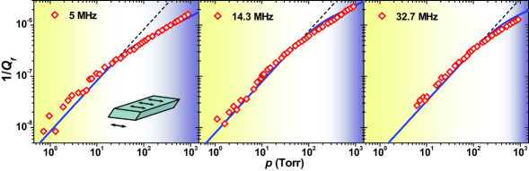
Figure 2: (color online). $1/Q_{f}$ in quartz crystal resonators at 5 MHz, 14.3 MHz and 32.7 MHz as a function of pressure. The inset is an illustration of the shear mode. The $\omega\tau\approx 1$ transition from non-Newtonian (yellow) to Newtonian (blue) flow takes place in the white regions at $p\approx$ 60, 200 and 400 Torr. The dotted lines are asymptotes proportional to $p$. The solid lines are fits to Eq. (8) using fitting factors 0.8, 0.6 and 0.9 and $S/m=2.754$ $\rm{m^{2}/kg}$, $9.827$ $\rm{m^{2}/kg}$ and $6.296$ $\rm{m^{2}/kg}$ (left to right).

Even more unexpected conclusions emerge for the unsteady flow generated by an infinite plate oscillating at (angular) frequency $\omega$ with peak velocity and amplitude $U$ and $A$, respectively (Fig. 1(b) and (c)) Stokes (1851). In the Newtonian limit $\omega\tau\ll 1$, the Stokes boundary layer thickness, $\delta=\sqrt{\frac{{2\nu}}{\omega}}$, is the only length scale in the problem. In this limit, ${\rm{Kn}}_{\delta}\propto\sqrt{{\rm{Wi}}}$ holds as above, since ${\rm{Kn}}_{\delta}=\frac{\lambda}{\delta}\approx\sqrt{\frac{{\omega\lambda^{2}}}{\nu}}\approx\sqrt{\omega\tau}$. Due to its geometric simplicity, this problem can be solved in the entire dimensionless frequency range $0<\omega\tau<\infty$ by a summation of the Chapman-Enskog expansion of kinetic theory Yakhot and Colosqui (2007); Karabacak et al. (2007) and non-perturbatively Chen et al. (2007). The analytic solution for the velocity field is obtained as

$$u_{x}(y)=Ue^{-y/\delta_{-}}\cos(\omega t-y/\delta_{+}),$$ (5)

with two new length scales, a wavelength $\delta_{+}$ and a penetration depth $\delta_{-}$:

$$\frac{\delta}{{\delta_{\pm}}}=(1+\omega^{2}\tau^{2})^{1/4}\left[\cos\left({\frac{{\tan^{-1}\omega\tau}}{2}}\right)\pm\right.$$

$$\left.\sin\left({\frac{{\tan^{-1}\omega\tau}}{2}}\right)\right].$$ (6)

In the limit $\omega\tau\gg 1$, $\delta$ disappears from the problem and $\delta_{-}$ becomes the relevant length scale. However, as $\omega\tau\to\infty$, the first Knudsen number saturates: ${\rm{Kn}}_{\delta_{-}}\equiv\frac{\lambda}{{\delta_{-}}}\to\frac{1}{2}$, indicating that in this limit ${\rm{Kn}}_{\delta_{-}}$ cannot appear as an expansion parameter in the stress-strain relation or as a scaling parameter in Eq. (3). The second Knudsen number, $\rm{Kn}_{\delta_{+}}\equiv\frac{\lambda}{{\delta_{+}}}\to\omega\tau$, becomes the exact same expansion parameter derived from the Chapman-Enskog expansion applied to the Boltzmann-BGK equation Yakhot and Colosqui (2007). We conclude that the only relevant scaling parameter for the oscillating plate problem valid in both Newtonian and non-Newtonian regimes is ${\rm{Wi}}=\omega\tau$, re-emphasizing that $\rm{Wi}$ does not contain any information about the linear dimensions of the oscillating body. Moreover, as long as $A\ll L$ and ${\mathop{\rm Re}\nolimits}\sim 0$, the flow over the oscillating body remains tangential along the surface, following the natural curvatures.

In order to provide experimental support for the predicted universality, we studied energy dissipation in flows generated by oscillating solid surfaces. For a large plate, the average energy dissipated per unit time can be obtained as $\dot{E}=\frac{{SU^{2}}}{2}f(\omega\tau)\sqrt{\frac{1}{2}\omega\mu\rho}$ by considering the shear stress on the plate. Here, $S$ is the surface area and $f(\omega\tau)$ is the scaling function found as Karabacak et al. (2007)

$$f(\omega\tau)=\frac{1}{{(1+\omega^{2}\tau^{2})^{3/4}}}\left[(1+\omega\tau)\cos\left({\frac{{\tan^{-1}\omega\tau}}{2}}\right)\right.$$

$$\left.-(1-\omega\tau)\sin\left({\frac{{\tan^{-1}\omega\tau}}{2}}\right)\right].$$ (7)

For a mechanical resonator with resonance frequency $\omega/2\pi$, the dissipation can be translated into a fluidic quality factor $Q_{f}$ from the relation

$$\frac{1}{Q_{f}}=\frac{{\dot{E}}}{{\omega E_{st}}}=\frac{S}{m}f(\omega\tau)\sqrt{\frac{{\mu\rho}}{{2\omega}}},$$ (8)

where $E_{st}=\frac{{mU^{2}}}{2}$ is the energy stored in the resonator with mode mass $m$. In a simple ideal gas, such as nitrogen at pressure $p$, $\tau\propto 1/p$ . $1/Q_{f}$ can then be expressed as a function of $p$ and follows two different asymptotes: $1/Q_{f}\propto p$ at low $p$ (non-Newtonian) and $1/Q_{f}\propto p^{1/2}$ at high $p$ (Newtonian). The transition between the asymptotes takes place at $\omega\tau\approx 1$, and shifts to higher $p$ as $\omega$ is increased since $\tau\propto 1/p$.

In our experiments, we measured the $Q$ factor of quartz crystals, microcantilevers and nanomechanical beams in dry nitrogen as a function of $p$ using electrical Lea et al. (1984) and optical techniques Karabacak et al. (2007). We excited the resonators at very small oscillation amplitudes ($A\ll L$) around their resonances. The energy losses arising both from the fluid and the resonator itself (coupled to the measurement circuit) determine the overall (loaded) quality factor as $1/Q_{l}=1/Q_{f}(p)+1/Q_{r}$. At low $p$, $1/Q_{f}\to 0$, allowing a measurement of $1/Q_{r}$, and subsequently, $1/Q_{f}(p)$ Karabacak et al. (2007).

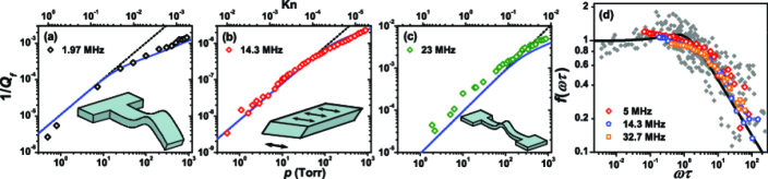
Figure 3: (color online). Fluidic dissipation across length scales. (a) A microcantilever with dimensions $l\times w\times t=$ 125 $\mu$m $\times$ 36 $\mu$m $\times$ 3.6 $\mu$m moving in its first flexural harmonic mode in the out-of-plane direction. (b) A quartz crystal of diameter 0.5 cm and thickness 0.1 mm moving in fundamental shear mode. (c) A nanomechanical doubly-clamped beam with $l\times w\times t=$ 17 $\mu$m $\times$ 500 nm $\times$ 280 nm moving in fundamental out-of-plane flexural mode. The upper axes in (a)-(c) show ${\rm{Kn}}=\lambda/L$ with $L\approx\sqrt{S}$. The dotted lines are asymptotes proportional to $p$ and the $\omega\tau\approx 1$ transition takes place at $p\approx$ 20, 200 and 300 Torr. All solid lines are obtained from theory. (d) Scaling of fluidic dissipation. The solid line shows the scaling function $f(\omega\tau)$ of Eq. (Universality in Oscillating Flows). The dissipation data of macroscopic quartz resonators are collapsed using Eq. (8) with the fitting factors and $S/m$ values mentioned in Fig. 2. The data points plotted in grey are from smaller flexural resonators of Karabacak et al. (2007). For the flexural resonators, the fitting factors are 2.8; $S/m$ values are calculated from geometry and mode shape Karabacak et al. (2007).

In Fig. 2, we show the basic aspects of the universality on similar sized macroscopic quartz crystals moving in fundamental shear mode (inset) at $\omega/2\pi=$ 5, 14.3 and 32.7 MHz. In each plot, the slope of $1/Q_{f}(p)$ changes due to the transition from non-Newtonian (yellow) to Newtonian (blue) flow. In order to fit the data to in Eq. (8), we used experimentally measured $S/m$ values and the recently suggested empirical form $\tau\approx\frac{{1.85\times 10^{-6}}}{p}$ ($\tau$ is in s when $p$ is in Torr) Karabacak et al. (2007). The flow for the small amplitude shear mode oscillations of the quartz crystals matches the large plate problem to a very good approximation Stockbridge (1966); Krim and Widom (1988). The only non-ideality may come from the velocity distribution on the surface of the resonator Martin and Hager (1989), which explains the small deviation of the fitting factors from unity.

The universality requires that the characteristics of the flow remain size and shape independent. We establish this aspect in Fig. 3(a)-(c) by comparing data on resonators, which span a broad range of linear dimension $L$ and oscillate in different modes: a macroscopic quartz crystal in shear-mode at 14.3 MH; a microcantilever and a nanomechanical doubly-clamped beam in flexural modes at 1.97 MHz and 23 MHz, respectively. We take the dynamically relevant linear dimension of the flow as $L\approx\sqrt{S}$, determined by the surface area. For the quartz crystal, $L_{Q}\approx{\rm{10}}^{{\rm{-2}}}$ ${\rm{m}}$, set by the electrode diameter Herrscher et al. (2007); Capelle et al. (1990). For the cantilever, $L_{C}\approx 10^{-4}$ $\rm{m}$ and for the beam, $L_{B}\approx 5\times 10^{-6}$ $\rm{m}$. The modes are illustrated in the insets; the flow remains tangential to the solid surface along the gentle curvatures. ${\rm{Kn}}=\lambda/L$ for the devices are shown on the upper axes. Two things are noteworthy: all curves look similar, and $L$ or $\rm{Kn}$ appears to have no effect on the flow in our parameter range Verbridge et al. (2008). Fig. 3(d) shows the dissipation data of macroscopic quartz resonators collapsed onto a dimensionless plot along with data of smaller resonators from Karabacak et al. (2007). In analyzing the data of flexural resonators, a fitting factor of 2.8 was used as opposed to the near unity fitting factors used for the shear-mode quartz crystals .

In our experiments, $\tau$ is determined by the microscopic interaction of gas molecules and a solid surface. By naively treating the nitrogen as a gas of hard spheres, one can obtain $\tau\approx\frac{{0.180\times 10^{-6}}}{p}$ ($\tau$ is in s when $p$ is in Torr). This value, however, only reflects interactions between gas molecules, as would happen away from surfaces in the bulk region of the gas. The observed dependence, which is roughly an order of magnitude larger, points to the importance of gas-surface interactions.

Our data provide evidence for a transition from purely viscous (Newtonian) to viscoelastic (non-Newtonian) dynamics in oscillating flows of simple gases in simple geometries. In our experiments, ${\mathop{\rm Re}\nolimits}\sim 0$ and non-linear effects, such as hydrodynamic instabilities and viscoelastic turbulence, are not present. The observed transition is due to the intrinsic dynamical response of the simple fluid to high-frequency perturbations. Similar observations are commonplace in macroscopic flows of concentrated long-chain polymer solutions, where $\tau$ can be long and, consequently, ${\rm{Wi}}\geq 1$ due to the relatively slow polymer dynamics Bird et al. (1987); Groisman and Steinberg (2000); Magda and Larson (1988). In rheology, polymers are often treated as elastic springs, and viscoelastic behavior of polymer solutions is attributed to the direct contribution of polymer molecules to the stress tensor. In this sense, our work points to a deep dynamical connection between oscillating flows of complex and simple fluids Bird et al. (1987).

We thank N. O. Azak, M. Y. Shagam and A. Vandelay for experimental help and discussions. This work was supported by Boston University through a Dean’s Catalyst Award and by the NSF through Grant No. CBET-0755927.

References

- Reynolds (1883) O. Reynolds, Phil. Trans. Roy. Soc. 174, 935 (1883).
- Landau and Lifshitz (1959) L. D. Landau and E. M. Lifshitz, Fluid Mechanics (Butterworth-Heinemann, Oxford, 1987), 2nd ed., pp. 56-58.
- Tanaka (1996) H. Tanaka, Phys. Rev. Lett. 76, 787 (1996).
- Landau and Lifshitz (1981) L. D. Landau and E. M. Lifshitz, Physical Kinetics (Butterworth-Heinemann, Oxford, 1981).
- Chen et al. (2004) H. Chen et al., J. Fluid Mechanics 519, 301 (2004).
- Cercignani (1975) C. Cercignani, Theory and application of the Boltzmann equation (Elsevier, New York, 1975).
- Squires and Quake (2005) T. Squires and S. R. Quake, Rev. Mod. Phys. 77, 977 (2005).
- Karabacak et al. (2007) D. M. Karabacak, V. Yakhot, and K. L. Ekinci, Phys. Rev. Lett. 98, 254505 (2007).
- Verbridge et al. (2008) S. S. Verbridge, et al., Appl. Phys. Lett. 93, 013101 (2008).
- Stroock et al. (2002) A. D. Stroock et al., Science 295, 647 (2002).
- Bird et al. (1987) R. B. Bird, R. C. Armstrong, and O. Hassager, Dynamics of polymeric liquids, Vol. 1 Fluid Mechanics, R. B. Bird, C. F. Curtis, R. C. Armstrong, and O. Hassager, Dynamics of polymeric liquids, Vol. 2 Kinetic Theory (John Wiley, New York, 1987).
- Groisman and Steinberg (2000) A. Groisman and V. Steinberg, Nature 405, 53 (2000).
- Wyss et al. (2007) H. M. Wyss et al., Phys. Rev. Lett. 98, 238303 (2007).
- Wang et al. (1999) X. Wang, X. Xu, and S. U. S. Choi, J. of Thermophysics and Heat Transfer 13, 474 (1999).
- Stokes (1851) G. G. Stokes, Trans. Cambridge Philos. Soc. 9, 8 (1851).
- Yakhot and Colosqui (2007) V. Yakhot and C. Colosqui, J. Fluid Mechanics 586, 249 (2007).
- Chen et al. (2007) H. Chen, S. A. Orszag, and I. Staroselsky, J. Fluid Mechanics 574, 495 (2007).
- Lea et al. (1984) M. J. Lea, P. Fozooni, and P. W. Retz, J. of Low Temp. Phys. 54, 303 (1984).
- Stockbridge (1966) C. D. Stockbridge, Vacuum Microbalance Techniques, vol. 5 (Plenum, New York, 1966).
- Krim and Widom (1988) J. Krim and A. Widom, Phys. Rev. B 38, 12184 (1988).
- Martin and Hager (1989) B. A. Martin and H. E. Hager, J. Appl. Phys. 65, 2630 (1989).
- Herrscher et al. (2007) M. Herrscher, C. Ziegler, and D. Johannsmann, J. Appl. Phys. 101, 114909 (2007).
- Capelle et al. (1990) B. Capelle et al., Proceedings of the 44th Annual Symposium on Frequency Control pp. 416–423 (1990).
- Magda and Larson (1988) J. J. Magda and R. G. Larson, J. Non-Newtonian Fluid Mech. 30, 1 (1988).