Q-systems, heaps, paths and cluster positivity

Abstract.

We consider the cluster algebra associated to the $Q$-system for $A_{r}$ as a tool for relating $Q$-system solutions to all possible sets of initial data. Considered as a discrete integrable dynamical system, we show that the conserved quantities are partition functions of hard particles on certain weighted graphs determined by the choice of initial data. This allows us to interpret the solutions of the system as partition functions of Viennot’s heaps on these graphs, or as partition functions of weighted paths on a dual graphs. The generating functions take the form of finite continued fractions. In this setting, the cluster mutations correspond to local rearrangements of the fractions which leave their final value unchanged. Finally, the general solutions of the $Q$-system are interpreted as partition functions for strongly non-intersecting families of lattice paths on target lattices. This expresses all cluster variables as manifestly positive Laurent polynomials of any initial data, thus proving the cluster positivity conjecture for the $A_{r}$ $Q$-system. We also give the relation to domino tilings of deformed Aztec diamonds with defects.

1. Introduction

The $A_{r}$ $Q$-system is a recursion relation satisfied by characters of special irreducible finite-dimensional modules of the Lie algebra $A_{r}$ [15]. It is a discrete integrable dynamical system. On the other hand, the relations of the $Q$-system are mutations in a cluster algebra defined in [14]. One of the goals of this paper is to prove the positivity property of the corresponding cluster variables, by using the integrability property.

We do this by solving the discrete integrable system, which can be mapped to several different types of statistical models: path models, heaps on graphs, or domino tilings. The choice initial conditions for the recursion relations determines the specific model, one for each choice of initial data. The Boltzmann weights are Laurent monomials in the initial data. Our construction gives an explicit solution of the $Q$-system as a function of any possible set of initial conditions.

It is a conjecture of Fomin and Zelevinsky [9] that the cluster variables at any seed $x$ of a cluster algebra, expressed as a function of the cluster variables of any other seed $y$ of the algebra, are Laurent polynomials with non-negative coefficients. In the language of dynamical systems, the choice of seed variables $y$ corresponds to the choice of initial conditions.

The methods used in this paper appear to be new in the context of the positivity conjecture. They have the advantage that they give explicit solutions, and extend immediately to $T$-systems [6] and to certain integrable non-commutative cluster algebras introduced by Kontsevich [16, 7].

1.1. The $Q$-system

First, let us recall some definitions. Let $I_{r}=\{1,...,r\}$, and consider the family of commutative variables $\{Q_{\alpha,n}~{}:~{}\alpha\in I_{r},n\in{\mathbb{Z}}\}$, related by a recursion relation of the form:

(1.1) $$Q_{\alpha,n+1}Q_{\alpha,n-1}=Q_{\alpha,n}^{2}-Q_{{\alpha}+1,n}Q_{{\alpha}-1,n},\quad Q_{0,n}=Q_{r+1,n}=1,\quad(n\in{\mathbb{Z}},~{}\alpha\in I_{r}).$$

A solution of this system is specified by giving a set of boundary conditions.

The original $A_{r}$ $Q$-system [15] is the recursion relation (1.1) (where $n\geq 1$), together with the boundary conditions

(1.2) $$Q_{\alpha,0}=1,\quad Q_{\alpha,1}={\rm ch}V(\omega_{\alpha}),\quad\alpha\in I_{r}.$$

Here, $V(\omega_{\alpha})$ is one of the $r$ fundamental representations of the Lie algebra $\mathfrak{sl}_{r+1}$. The solutions, written as functions of the initial variables, are the characters of the $A_{r}$ Kirillov-Reshetikhin modules [15]:

$$Q_{{\alpha},n}={\rm ch}V(n\omega_{\alpha}).$$

The boundary conditions (1.2) are singular, in that $Q_{\alpha,-1}=0$. All solutions are therefore polynomials in $\{Q_{{\alpha},1}:{\alpha}\in I_{r}\}$ (Lemma 4.2 of [4]). In this paper, we relax this boundary condition. Moreover, as we are interested in the positivity property of cluster algebras, we renormalize the variables in (1.1). Let

(1.3) $$R_{\alpha,n}=\epsilon_{\alpha}Q_{\alpha,n},\qquad\epsilon_{\alpha}=e^{i\pi\sum_{\beta=1}^{r}(C^{-1})_{\alpha,\beta}}=e^{i\pi\alpha(r+1-\alpha)/2}$$

where $C$ the Cartan matrix of $A_{r}$. Then

(1.4) $$R_{\alpha,n+1}R_{\alpha,n-1}=R_{\alpha,n}^{2}+R_{{\alpha}+1,n}R_{{\alpha}-1,n},\quad R_{0,n}=R_{r+1,n}=1,\quad(\alpha\in I_{r},~{}n\in{\mathbb{Z}}).$$

In the rest of the paper we work only with the renormalized variables in (1.3), and henceforth we refer to Equation 1.4 as the $A_{r}$ $Q$-system.

1.2. $Q$-systems as Cluster algebras

Instead of specifying the boundary conditions of the form (1.2), we may specify much more general boundary conditions by picking a set $2r$ variables in a consistent manner, and setting them to be formal variables. Any solution is then a function of these formal variables. In order to explain what we mean by “a consistent manner”, we can use the formulation of these recursion relations as mutations in a cluster algebra.

It was shown in [14] that the system (1.4) can be expressed in terms of a cluster algebra [9]:

Theorem 1.1.

[14] The equations (1.4) for each ${\alpha}$ and $n$ are mutations in the cluster algebra without coefficients, of rank $2r$, defined by the seed $({\mathbf{x}}_{0},B_{0})$, where ${\mathbf{x}}_{0}$ is a cluster variable and $B_{0}$ is an exchange matrix, with

(1.5) $${\mathbf{x}}_{0}=(R_{1,0},...,R_{r,0};R_{1,1},...,R_{r,1}),\quad B_{0}=\left(\begin{array}[]{cc}0&-C\\ C&0\end{array}\right),$$

where $C$ is the Cartan matrix of $A_{r}$.

A cluster algebra of rank $n$ without coefficients is defined as follows [9]. Consider an an $n$-regular tree $\mathbb{T}_{n}$, with nodes connected via labeled edges. Each node is attached to $n$ edges with distinct labels $1,...,n$. To each node $t$, we associate a seed consisting of a cluster variable and an exchange matrix. The cluster variable $\mathbf{x}_{t}$ has $n$ components, $\mathbf{x}_{t}=(x_{t,0},...,x_{t,n}),$ and the exchange matrix $B_{t}$ is an $n\times n$ skew-symmetric matrix.

Cluster variables at connected nodes are related by mutations given by the exchange matrix. Suppose node $t$ is connected to node $t^{\prime}$ by an edge labeled $k$, then the seeds at these nodes are related by a mutation $\mu_{k}$. The effect of this mutation is as follows:

$$\mu_{k}(x_{t,j}) = x_{t^{\prime},j}=\left\{\begin{array}[]{ll}x_{t,j}^{-1}\left(\prod_{i=1}^{n}x_{t,i}^{[(B_{t})_{ij}]_{+}}+\prod_{i=1}^{n}x_{t,i}^{[-(B_{t})_{ij}]_{+}}\right),&k=j\\ x_{t,j}&\hbox{otherwise}.\end{array}\right.$$

Here, $[n]_{+}={\rm max}(0,n)$. The matrices $B_{t}$ and $B_{t^{\prime}}$ are related via the mutation $\mu_{k}$ as follows.

(1.8) $$\mu_{k}((B_{t}))_{ij} = \left\{\begin{array}[]{ll}-(B_{t})_{ij}&\hbox{if $i=k$ or $j=k$,}\\ (B_{t^{\prime}})_{ij}=(B_{t})_{ij}+{\rm sign}((B_{t})_{ik})[(B_{t})_{ik}(B_{t})_{kj}]_{+}&\hbox{otherwise}\end{array}\right.$$

The cluster algebra is the commutative algebra over ${\mathbb{Q}}$ of the cluster variables.

In the case of the cluster algebra defined in Theorem 1.1, there is a subgraph $\mathcal{G}_{r}$ of $\mathbb{T}_{2r}$, which includes the node with seed (1.5), and is the maximal subgraph with the property that the mutation of the cluster variables along each edge of the graph is one of the equations (1.4). The union of the cluster variables over all nodes of the graph is the set $\{R_{\alpha,n}:\alpha\in I_{r},n\in{\mathbb{Z}}\}$.

To describe the seeds in $\mathcal{G}_{r}$, note that the mutation of the variable $R_{{\alpha},n-1}$ into $R_{{\alpha},n+1}$ uses the variables $\{R_{{\alpha},n-1},R_{{\alpha}-1,n},R_{{\alpha},n},R_{{\alpha}+1,n}\}$. If these are entries of the cluster variable ${\mathbf{x}}_{t}$ at node $t$, then it is possible to apply the mutation $t\to t^{\prime}$ which sends $R_{{\alpha},n-1}\to R_{{\alpha},n+1}$. With our indexing convention, this is the mutation $\mu_{\alpha}$ if $n$ is odd, $\mu_{{\alpha}+r}$ if $n$ is even. Such a mutation will be called a “forward” mutation, as it increases the value of the index $n-1\to n+1$. (Cluster mutations are involutions, hence we also have “backward” mutations which send $n+1\to n-1$.)

We see that any cluster variable in $\mathcal{G}_{r}$ has the properties: (i) The variable consists of pairs the form $(R_{{\alpha},m_{\alpha}},R_{{\alpha},m_{\alpha}+1})$, ${\alpha}\in I_{r}$ and (ii) $m_{{\alpha}-1}-1\leq m_{\alpha}\leq m_{{\alpha}-1}+1$ for all ${\alpha}\in I_{r}$. Define a path on the two-dimensional lattice in the $(n,{\alpha})$-plane, by connecting the points ${\mathbf{M}}=\{(m_{\alpha},{\alpha})\}_{{\alpha}=1}^{r}$. Then condition (ii) implies that ${\mathbf{M}}$ is a Motzkin path, with steps of type $(1,1)$, $(-1,1)$ and $(0,1)$. Therefore we have

Lemma 1.2.

The nodes of ${\mathcal{G}}_{r}$ are in bijection with Motzkin paths on the square lattice with $r-1$ steps of the form $(1,1)$, $(-1,1)$ or $(0,1)$, connecting vertices with integer coordinates $(n,{\alpha})$ such that $1\leq{\alpha}\leq r$.

We define ${\mathbf{x}}_{\mathbf{M}}$ to be the seed with the variables $\{R_{{\alpha},m_{\alpha}+i}:i=0,1,{\alpha}\in I_{r}\}$. Let ${\mathbf{M}}_{0}$ denote the Motzkin path with $m_{\alpha}=0$, ${\alpha}\in I_{r}$. Then ${\mathbf{x}}_{0}={\mathbf{x}}_{{\mathbf{M}}_{0}}$. Forward mutations $\mu_{\alpha}$ and $\mu_{{\alpha}+r}$ act on Motzkin paths by increasing or decreasing one of the indices $m_{\alpha}$. If the resulting path is also a Motzkin path, such mutations are guaranteed to be of the type (1.4).

The graph $\mathcal{G}_{r}$ is an infinite strip, and we display a section of it for $r=3$ in Figure 1, where we have identified the nodes sharing the same cluster variables. Most of the results of this paper can be reduced to working with the fundamental domain of this strip.

Figure 1. The subgraph of $Q$-system mutations for $A_{3}$. The blue dot stands for the node $0$.

1.3. Outline of the paper

The Laurent property [10] guarantees that the cluster variables are Laurent polynomials when expressed as functions of the cluster variables of any seed in the cluster algebra. It is a general conjecture [9] that the coefficients of the monomials in these Laurent polynomials are non-negative integers. In this paper, we prove positivity for the cluster variables in $\mathcal{G}_{r}$.

The $Q$-system is a way of relating the solutions of (1.4) to all possible sets of initial data. Mutations of the cluster algebra allow us to move within the set of possible initial data, as long as this initial data is of the form ${\mathbf{x}}_{\mathbf{M}}$. Our aim is to give an explicit combinatorial description of $R_{{\alpha},n}$, for each choice of initial data ${\mathbf{x}}_{\mathbf{M}}$ within this set, as the partition function for a statistical model with positive Boltzmann weights.

We proceed using the following steps:

Step 1. We give a combinatorial description of $\{R_{1,n},~{}n\in{\mathbb{Z}}\}$ as functions of the initial data ${\mathbf{x}}_{0}$. All other variables $\{R_{{\alpha},n},~{}{\alpha}>1\}$ are discrete Wronskians of $\{R_{1,n+j},~{}1-{\alpha}\leq j\leq{\alpha}-1\}$. The variables $\{R_{1,n},~{}n\in{\mathbb{Z}}\}$ satisfy a linear recursion relation with constant coefficients, which are the conserved quantities of the $Q$-system. Here, the integrability of the system plays a crucial role.

The conserved quantities are partition functions of hard particles on a weighted graph $G_{r}$, with weights which are Laurent monomials in the cluster variables ${\mathbf{x}}_{0}$. Therefore the generating function $F_{1}^{(r)}(t)=\sum_{n\geq 0}t^{n}R_{1,n}$ is equal to the partition function of Viennot’s heaps on $G_{r}$. Thus, there is a simple expression for $F_{1}^{(r)}(t)$ as a finite continued fraction.

Elementary rearrangements of the continued fraction allow us to express $F_{1}^{(r)}(t)$ as the generating function for heaps on different graphs with different weights. Our goal is then to prove that these rearrangements are mutations of the initial data ${\mathbf{x}}_{{\mathbf{M}}}$.

Step 2. We use a heap-path correspondence to re-express $\{R_{1,n}({\mathbf{x}}_{0})\}_{n\in{\mathbb{Z}}_{+}}$ as partition functions for weighted paths on a dual graph ${\widetilde{G}}_{r}$.

Step 3. For each Motzkin path ${\mathbf{M}}$, we construct a graph $\Gamma_{\mathbf{M}}$ and edge weights $y_{e}({\mathbf{M}})$ which are Laurent monomials in the cluster variables ${\mathbf{x}}_{\mathbf{M}}$. The variables $\{R_{1,n}\}_{n\in{\mathbb{Z}}_{+}}$ are expressed as the generating functions for weighted paths on $\Gamma_{\mathbf{M}}$. This proves the positivity conjecture for $R_{1,n}$ and the claim that continued fraction rearrangements are cluster mutations of initial data.

Step 4. We use the discrete Wronskian expression for $R_{{\alpha},n}$ to interpret these variables as partition functions for families of strongly non-intersecting paths on $\Gamma_{\mathbf{M}}$. This is done by a generalization of the Lindström-Gessel-Viennot [19, 11] determinant formula for the counting of non-intersecting lattice paths. This implies the positivity property for $R_{{\alpha},n}$ as functions of ${\mathbf{x}}_{\mathbf{M}}$.

The paper is organized as follows. In Section 2, we show that the $Q$-system amounts to a discrete Wronskian equation for the $R_{1,n}$’s, and that $R_{{\alpha},n}$ with ${\alpha}>1$ are expressed as ${\alpha}\times{\alpha}$ discrete Wronskians of $R_{1,n}$. We deduce that $R_{1,n}$ satisfies a linear recursion relation with constant coefficients, interpreted as the conserved quantities of the $Q$-system.

In Section 3, the conserved quantities are interpreted as partition functions for hard particles on a certain target graph $G_{r}$, with vertex weights which depend on the initial data ${\mathbf{x}}_{0}$ of (1.5). We rephrase the linear recursion relation for $R_{1,n}$ in terms of generating functions which are simple rational functions.

In Section 4 we re-interpret these rational functions as partition functions for Viennot’s heaps [24] on the same target graph $G_{r}$. This gives a first proof of the positivity of $R_{1,n}$ as a Laurent polynomial of the initial data ${\mathbf{x}}_{0}$ (1.5). We also give an explicit expression for the generating function of $R_{1,n}$’s, as a finite continued fraction. We show how a simple rearrangement lemma for fractions allows, by iterative use, to rewrite the partition function for heaps on $G_{r}$ as a partition function for heaps on other graphs, with weights accordingly transformed. The proof that these rearrangements correspond to mutations of the cluster variables appears in Section 6.

In Section 5 we reformulate the heap partition function in terms of weighted paths on “dual” target graphs, the language of which is more amenable to mutations. For each Motzkin path, we construct a corresponding graph with edge weights which are monomials in ${\mathbf{x}}_{\mathbf{M}}$. Partition functions for paths on these graphs are the cluster variables $R_{1,n}$. For completeness, we also explain how to construct the dual graphs for the heap models from these graphs.

In Section 6 we prove that $R_{1,n}$ is the partition function for weighted paths on a target graph $\Gamma_{\mathbf{M}}$ with weights determined by the initial data ${\mathbf{x}}_{\mathbf{M}}$. Using the transfer matrix formulation, we prove the statement that fraction rearrangements correspond to mutations of the initial data. This leads to the main positivity theorem for the cluster variables $R_{1,n}$, in terms of any initial data ${\mathbf{x}}_{\mathbf{M}}$.

The extension of this result to $R_{{\alpha},n}$, ${\alpha}>1$ is presented in Section 7, where $R_{{\alpha},n}$ is interpreted à la Lindström-Gessel-Viennot as the partition function for families of strongly non-intersecting weighted paths on the same target graph as for $R_{1,n}$. This completes the statistical-mechanical interpretation of all the solutions of the $Q$-system, and proves the positivity of all the cluster variables of the subgraph corresponding to the $Q$-system, when expressed in terms of cluster variables at any of its nodes.

In Section 8 we discuss the limiting case of $A_{\infty/2}$ and present various exact and asymptotic path enumeration results, which correspond to picking initial data $x_{\mathbf{M}}$ with entries all equal to $1$.

Finally, since the $Q$-system is a limit of the $T$-system, aka the octahedron equation, in Section 9 we give the relation of our results to the known results on the octahedron equation. We show how to relate weighted domino tilings of the Aztec diamond to our weighted non-intersecting families of lattice paths, and to interpret the result of cluster mutations in that language as weighted tilings of suitably deformed Aztec diamonds, by means of dominos and also pairs of square “defects”.

The appendices include explicit examples of our constructions for the case $A_{3}$.

Acknowledgements: We thank M. Bergvelt, C. Krattenthaler, A. Postnikov, H. Thomas, and particularly S. Fomin for many interesting discussions. We thank the organizers of the semester “Combinatorial Representation Theory” and the Mathematical Science Research Institute, Berkeley, CA, USA for hospitality, as well as the organizers of the program “Combinatorics and Statistical Physics” and the Erwin Schrödinger International Institute for Mathematical Physics, Vienna, Austria. R.K. acknowledges the hospitality of the Institut des Hautes Etudes Scientifiques, Bures-sur-Yvette, France. P. D.F. acknowledges the support of the ENIGMA research training network MRTN-CT-2004-5652, the ANR program GIMP, and the ESF program MISGAM. R. K.’s research is supported by NSF grants DMS 0500759 and 0802511.

2. Properties of the $Q$-system

2.1. The fundamental domain of seeds

Our goal is give explicit expressions for $R_{{\alpha},n}$ as a function of any initial seed data ${\mathbf{x}}_{{\mathbf{M}}}$. First, we use the symmetries of the $Q$-system to enable us to restrict our attention to a finite fundamental domain of initial seeds, parametrized by Motzkin paths which have a minimum node at $0$.

There are three obvious symmetries of the system. A symmetry $\sigma:\{R_{{\alpha},n}\}\to\{R_{{\alpha},n}\}$ of (1.4) is a map with the property that $R_{{\alpha},n}=f({\mathbf{x}})$ then $\sigma(R_{{\alpha},n})=f(\sigma({\mathbf{x}}))$. Equation (1.4) is invariant under $\sigma(R_{\alpha,n})=R_{\alpha,-n+1}$. Therefore,

Lemma 2.1.

“Time reversal”:

$${\rm if}\ R_{{\alpha},n} = f(R_{1,0},R_{2,0},...,R_{r,0};R_{1,1},R_{2,1},...,R_{r,1}),$$

(2.1) $${\rm then}\ R_{{\alpha},-n+1} = f(R_{1,1},R_{2,1},...,R_{r,1};R_{1,0},R_{2,0},...,R_{r,0}).$$

for all $n\in{\mathbb{Z}}$ and ${\alpha}\in I_{r}$.

We also have the reflection symmetry of (1.4), $\sigma(R_{{\alpha},n})=R_{r+1-{\alpha},n}$. Therefore,

Lemma 2.2.

$${\rm if}\ R_{{\alpha},n} = f(R_{1,0},R_{2,0},...,R_{r,0};R_{1,1},R_{2,1},...,R_{r,1})$$

(2.2) $${\rm then}\ R_{r+1-{\alpha},n} = f(R_{r,0},R_{r-1,0},...,R_{1,0};R_{r,1},R_{r-1,1},...,R_{1,1}).$$

for all $n\in{\mathbb{Z}}$ and ${\alpha}\in I_{r}$.

Finally, we have the translational invariance, $\sigma(R_{{\alpha},n})=R_{{\alpha},n+k}$:

Lemma 2.3.

$${\rm if}\ R_{{\alpha},n} = f(R_{1,0},R_{2,0},...,R_{r,0};R_{1,1},R_{2,1},...,R_{r,1}),$$

(2.3) $${\rm then}\ R_{{\alpha},n+k} = f(R_{1,k},R_{2,k},...,R_{r,k};R_{1,k+1},R_{2,k+1},...,R_{r,k+1}).$$

for all $n,k\in{\mathbb{Z}}$ and ${\alpha}\in I_{r}$.

This lemma may also be viewed as a special case of the substitution property of deformed $Q$-systems defined in [3].

For any Motzkin path ${\mathbf{M}}=(m_{1},...,m_{r})$, let $f_{{\alpha},n}^{({\mathbf{M}})}({\mathbf{x}})$ denote the function of ${\mathbf{x}}$ such that

$$R_{{\alpha},n}=f_{{\alpha},n}^{({\mathbf{M}})}({\mathbf{x}}_{\mathbf{M}}).$$

Let ${\mathbf{M}}+k=(m_{1}+k,...,m_{r}+k)$. Then Equation (2.3) can be written as

(2.4) $$R_{{\alpha},n}=f_{{\alpha},n}^{({\mathbf{M}}_{0})}({\mathbf{x}}_{{\mathbf{M}}_{0}})=f_{{\alpha},n-k}^{({\mathbf{M}}_{0})}({\mathbf{x}}_{{\mathbf{M}}_{0}+k}).$$

More generally,

(2.5) $$R_{{\alpha},n+k}=f_{{\alpha},n+k}^{({\mathbf{M}})}({\mathbf{x}}_{{\mathbf{M}}})=f_{{\alpha},n+k}^{({\mathbf{M}}_{0})}({\mathbf{x}}_{{\mathbf{M}}_{0}})=f_{{\alpha},n}^{({\mathbf{M}}_{0})}({\mathbf{x}}_{{\mathbf{M}}_{0}+k})=f_{{\alpha},n}^{({\mathbf{M}})}({\mathbf{x}}_{{\mathbf{M}}+k}).$$

Therefore,

Theorem 2.4.

Let $R_{{\alpha},n}=f_{{\alpha},n}^{({\mathbf{M}})}({\mathbf{x}}_{\mathbf{M}})$, where $f_{{\alpha},n}^{({\mathbf{M}})}$ is a positive Laurent polynomial of ${\mathbf{x}}_{\mathbf{M}}$, ${\alpha}\in I_{r}$, $n\in{\mathbb{Z}}$. Then as a function of ${\mathbf{x}}_{{\mathbf{M}}+k}$, $k\in{\mathbb{Z}}$, $R_{{\alpha},n}$ is also a positive Laurent polynomial, $R_{{\alpha},n}=f_{{\alpha},n}^{({\mathbf{M}}+k)}({\mathbf{x}}_{{\mathbf{M}}+k})$.

We can thus restrict our attention to fundamental domain:

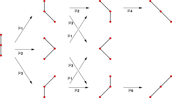
Figure 2. The Motzkin paths for the 9 seeds in the fundamental domain for the $A_{3}$ case, and the mutations relating them. The leftmost vertices of each Motzkin path lie on the vertical axis $x=0$.

Definition 2.5.

The fundamental domain ${\mathcal{F}}_{r}$ for the $A_{r}$ $Q$-system is indexed by the Motzkin paths with $r-1$ steps of the form $\{(m_{\alpha},{\alpha})\}_{{\alpha}\in I_{r}}$, with Min${}_{{\alpha}\in I_{r}}(m_{\alpha})=0$.

There are exactly $3^{r-1}$ Motzkin paths in the fundamental domain. As an example, Figure 2 shows the $9$ Motzkin paths of the fundamental domain for $A_{3}$ and the mutations relating them, c.f. the graph ${\mathcal{G}}_{3}$ in Figure 1.

2.2. Discrete Wronskians

For any matrix $M$, let $M_{i_{1},...,i_{k}}^{j_{1},...,j_{m}}$ be the matrix obtained by it by removing rows $i_{1},...,r_{k}$ and columns $j_{1},...,j_{m}$.

2.2.1. Plücker relations

Let $T$ be an $n\times(n+k)$-matrix. The Plücker relations for the minors of $T$ are

(2.6) $$|T^{a_{1},...,a_{k}}|\,|T^{b_{1},...,b_{k}}|=\sum_{p=1}^{k}|T^{b_{p},a_{2}...,a_{k}}|\,|T^{b_{1},...,b_{p-1},a_{1},b_{p+1},...,b_{k}}|.$$

In particular, when $k=2$,

(2.7) $$|T^{a_{1},a_{2}}|\,|T^{b_{1},b_{2}}|=|T^{b_{1},a_{2}}|\,|T^{a_{1},b_{2}}|+|T^{b_{2},a_{2}}|\,|T^{b_{1},a_{1}}|.$$

Let $n=r+1$, $a_{2}=j_{1}$, $b_{2}=j_{2}$, and $(T)_{i,a_{1}}=\delta_{i,i_{1}}$, $(T)_{i,b_{1}}=\delta_{i,i_{2}}$. Then Equation (2.7) gives the Desnanot-Jacobi formula for the minors of the matrix $M=T^{a_{1},b_{1}}$ of size $(r+1)\times(r+1)$:

(2.8) $$|M|\,|M_{i_{1},i_{2}}^{j_{1},j_{2}}|=|M_{i_{1}}^{j_{1}}|\,|M_{i_{2}}^{j_{2}}|-|M_{i_{1}}^{j_{2}}|\,|M_{i_{2}}^{j_{1}}|.$$

2.2.2. Wronskian formula for $R_{1,n}$

Using (1.4), it is possible to eliminate the variables $\{R_{\alpha,n}\}_{\alpha>1}$ in favor of $\{R_{1,n}\}$. The remaining equations determine $\{R_{1,n}\}$ in terms of the initial data. As a consequence, $R_{1,n}$ satisfies a linear recursion relation with constant coefficients. This can then be extended trivially to all $R_{\alpha,n}$.

Define the ${\alpha}\times{\alpha}$ matrix $M_{{\alpha},n}$ with $(M_{\alpha,n})_{i,j}=R_{1,n+i+j-1-\alpha}$. That is,

(2.9) $$M_{{\alpha},n}=\left(\begin{matrix}R_{1,n-\alpha+1}&R_{1,n-\alpha+2}&\cdots&R_{1,n}\cr R_{1,n-\alpha+2}&R_{1,n-\alpha+3}&\cdots&R_{1,n+1}\cr\vdots&\vdots&\ddots&\vdots\cr R_{1,n}&R_{1,n+1}&\cdots&R_{1,n+\alpha-1}\end{matrix}\right).$$

and define the discrete Wronskian determinant to be $W_{{\alpha},n}=|M_{{\alpha},n}|$.

Lemma 2.6.

We have $R_{\alpha,n}=W_{\alpha,n}$.

Proof.

Applying the Desnanot-Jacobi formula (2.8) to the $({\alpha}+1)\times({\alpha}+1)$ matrix $M$ with entries

$$(M)_{i,j}=R_{1,n+i+j-{\alpha}-2}$$

with the choice of rows $i_{1}=1,i_{2}={\alpha}+1$, and columns $j_{1}=1$, $j_{2}={\alpha}+1$, we have

(2.10) $$W_{\alpha,n+1}W_{\alpha,n-1}=W_{\alpha,n}^{2}+W_{\alpha+1,n}W_{\alpha-1,n}$$

for any sequence $R_{1,n}$, and any $\alpha\geq 1$, with the convention that $W_{0,n}=1$ for all $n$. The sequence $W_{{\alpha},n}$ is the unique solution to eq.(2.10) such that $W_{0,n}=1$ and $W_{1,n}=R_{1,n}$. Comparing this to the Q-system (1.4), we deduce that $R_{\alpha,n}=W_{\alpha,n}$, ${\alpha}=1,...,r$, and the Lemma follows. ∎

The boundary condition $R_{r+1,n}=1$ yields the following polynomial relation for $R_{1,n}$:

Corollary 2.7.

(2.11) $$W_{r+1,n}=\left|\begin{matrix}R_{1,n-r}&R_{1,n-r+1}&\cdots&R_{1,n}\cr R_{1,n-r+1}&R_{1,n-r+2}&\cdots&R_{1,n+1}\cr\vdots&\vdots&\ddots&\vdots\cr R_{1,n}&R_{1,n+1}&\cdots&R_{1,n+r}\end{matrix}\right|=1.$$

2.2.3. Integrals of motion

The determinant $W_{r+1,n}$ is a discrete version of the Wronskian determinant $W(f_{1},...,f_{r})=\det_{i,j}(f_{i}^{(j-1)})$. In the theory of linear differential equations, the Wronskian of $r$ linearly independent solutions to an $r$-th order linear differential equation is a constant. This is proved by differentiating the Wronskian and noting that a linear combination of its columns vanishes, due to the differential equation. Conversely, if the Wronskian is a (non-zero) constant (so that its columns are linearly independent), there exists a vanishing linear combination between the column vectors of its derivative, namely $f_{i}^{(r)}=\sum_{j=1}^{r-1}a_{j}f_{i}^{(j-1)}$, where the $f$’s are a linearly independent set of solutions of these equations.

Theorem 2.8.

The variables $\{R_{1,n}\}_{n\in{\mathbb{Z}}}$ satisfy a linear recursion relation involving $r+2$ terms:

(2.12) $$\sum_{m=0}^{r+1}(-1)^{m}c_{r+1-m}R_{1,n+m}=0,\quad n\in{\mathbb{Z}},$$

with the coefficients $c_{0}=c_{r+1}=1$, and with $c_{1},c_{2},...,c_{r}$ some constant (independent of $n$) coefficients determined by the initial conditions.

Proof.

In analogy with the continuous situation, consider the discrete derivative $W_{r+1,n+1}-W_{r+1,n}=0$. Since $W_{r+1,n}$ and $W_{r+1,n+1}$ have $r$ identical columns ($(W_{r+1,n+1})_{i,j}=(W_{r+1,n})_{i+1,j}$, $i\in I_{r}$),

(2.13) $$W_{r+1,n+1}-W_{r+1,n}=\det_{1\leq i,j\leq r+1}\left(R_{1,n+i+j-r-1}-(-1)^{r}\delta_{j,r+1}R_{1,n+i-r-1}\right)=0.$$

As a consequence, there exists a non-trivial linear combination of the columns of this difference which vanishes. From the form of the entries of these columns (in which the indices are shifted by $-1$ relative to each other) the coefficients of this linear combination are independent of $n$. ∎

3. Conserved quantities and Hard Particles

3.1. Conserved quantities of the Q-system

Since $W_{r+1,n}=1$, it is a conserved quantity, i.e. it is independent of $n$. More generally, we claim that there are $r+1$ linearly independent conserved quantities, and therefore the $Q$-system is a discrete integrable system in the Liouville sense.

Theorem 3.1.

The following polynomials

$$c_{i-1}=|(M_{r+2,n})_{r+2}^{r+2-i}|,\quad i=0,...,r$$

where $c_{r+1}=c_{0}=1$, are independent of $n$, and $c_{0},...,c_{r}$ are the linearly independent conserved quantities of the $A_{r}$ $Q$-system.

Proof.

This follows from the fact that $W_{r+2,n}=0$, as a consequence of the boundary condition $W_{r+1,n}=1$ and the $Q$-system relation. The conserved quantities are the minors of the expansion of this determinant with respect to the last row, as in Equation (2.12). We get only $r+1$ linearly independent minors, since $c_{0}=W_{r+1,k-1}=1=W_{r+1,k}=c_{r+1}$. ∎

Example 3.2.

For $r=1$, we have

$$c_{1}=\left|\begin{matrix}R_{1,k-2}&R_{1,k}\\ R_{1,k-1}&R_{1,k+1}\end{matrix}\right|={R_{1,1}\over R_{1,0}}+{1\over R_{1,0}R_{1,1}}+{R_{1,0}\over R_{1,1}}.$$

Using the Q-system for $A_{1}$ to eliminate $R_{1,k+2}=(R_{1,k+1}^{2}+1)/R_{1,k-1}$ and $R_{1,k-2}=(R_{1,k+1}^{2}+1)/R_{1,k-1}$, we get the conservation law:

$$c_{1}={R_{1,k}\over R_{1,k-1}}+{1\over R_{1,k-1}R_{1,k}}+{R_{1,k-1}\over R_{1,k}}={R_{1,1}\over R_{1,0}}+{1\over R_{1,0}R_{1,1}}+{R_{1,0}\over R_{1,1}}.$$

This is a two-term recursion relation in $k$, whereas the $Q$-system is a three-term recursion. The former is an explicit discrete “first integral” of the latter.

Another way of understanding the conserved quantities of Theorem 3.1 is via the translational invariance of the cluster algebra, expressed in Lemma 2.3. We get the following immediate

Corollary 3.3.

The quantities $c_{i}$, expressed in terms of the seed ${\mathbf{x}}_{0}$, are conserved, namely:

(3.1) $$c_{i}(R_{1,0},\ldots,R_{r,0};R_{1,1},\ldots,R_{r,1})=c_{i}(R_{1,k},\ldots,R_{r,k};R_{1,k+1},\ldots,R_{r,k+1})$$

for all $k\in{\mathbb{Z}}$ and for $i=0,1,2,...,r$.

3.2. Recursion relations for discrete Wronskians with defects

We now derive explicit relations between the $c_{i}$ and the initial data. It is useful to work in the context of the $A_{\infty/2}$ $Q$-system, which is obtained from the $A_{r}$ system by relaxing the boundary condition $R_{r+1,n}=1$:

(3.2) $$r_{{\alpha},n+1}r_{{\alpha},n-1}=r_{{\alpha},n}^{2}+r_{{\alpha}+1,n}r_{{\alpha}-1,n},\ \ \ r_{0,n}=1,n\in{\mathbb{Z}},{\alpha}\geq 1.$$

Again, as in Lemma 2.6, we have

$$r_{{\alpha},n}:=\det_{1\leq i,j\leq{\alpha}}(r_{1,n+i+j-1-{\alpha}}).$$

Define the ${\alpha}\times{\alpha}$ Wronskians with a “defect” at position ${\alpha}-m$ ($0\leq m\leq{\alpha}$, $n\in{\mathbb{Z}}$):

(3.3) $$c_{{\alpha},m,n}=\det_{1\leq i,j\leq{\alpha}}\,r_{1,n+i+s_{{\alpha}-m}(j)-{\alpha}-1},\qquad s_{m}(j)=\left\{\begin{matrix}j&{\rm if}\ j\leq m\\ j+1&{\rm if}\ j>m\end{matrix}\right.$$

where $c_{0,0,n}=1$ for all $n$. Note that $c_{{\alpha},0,n}=r_{{\alpha},n}$ and $c_{{\alpha},{\alpha},n}=r_{{\alpha},n+1}$. In addition, $c_{i}=c_{r+1,i,k}$ if $r_{{\alpha},n}=R_{{\alpha},n}$, that is, when we impose the condition $r_{r+1,n}=1$.

Lemma 3.4.

The $c_{{\alpha},m,n}$ satisfy the following recursion relation:

(3.4) $$r_{{\alpha}-1,n}r_{{\alpha}-1,n+1}c_{{\alpha},m,n}=r_{{\alpha},n}r_{{\alpha}-1,n+1}c_{{\alpha}-1,m,n}+r_{{\alpha}-1,n}r_{{\alpha},n+1}c_{{\alpha}-1,m-1,n}+r_{{\alpha},n}r_{{\alpha},n+1}c_{{\alpha}-2,m-1,n}.$$

Proof.

Applying (2.8) to the ${\alpha}\times{\alpha}$ matrix $M$ with entries $M_{i,j}=r_{1,n+i+j-{\alpha}}$, $i,j\in\{1,\ldots,\alpha\}$, with $i_{1}=1$, $i_{2}={\alpha}$, $j_{1}={\alpha}-m$ and $j_{2}={\alpha}$,

(3.5) $$r_{{\alpha},n+1}c_{{\alpha}-2,m-1,n}+r_{{\alpha}-1,n+1}c_{{\alpha}-1,m,n}=r_{{\alpha}-1,n}c_{{\alpha}-1,m,n+1}.$$

Using this to simplify the sum of the first and last terms on the r.h.s. of (3.4), must prove that

(3.6) $$r_{{\alpha}-1,n+1}c_{{\alpha},m,n}=r_{{\alpha},n+1}c_{{\alpha}-1,m-1,n}+r_{{\alpha},n}c_{{\alpha}-1,m,n+1}.$$

Multiplying (3.6) by $r_{{\alpha},n+1}$, and using (3.2),

$$r_{{\alpha},n+1}r_{{\alpha}-1,n+1}c_{{\alpha},m,n}-(r_{{\alpha},n+2}r_{{\alpha},n}-r_{{\alpha}+1,n+1}r_{{\alpha}-1,n+1})c_{{\alpha}-1,m-1,n}-r_{{\alpha},n+1}r_{{\alpha},n}c_{{\alpha}-1,m,n+1}$$

$$= r_{{\alpha}-1,n+1}(r_{{\alpha},n+1}c_{{\alpha},m,n}+r_{{\alpha}+1,n+1}c_{{\alpha}-1,m-1,n})-r_{{\alpha},n}(r_{{\alpha},n+2}c_{{\alpha}-1,m-1,n}+r_{{\alpha},n+1}c_{{\alpha}-1,m,n+1})$$

$$= r_{{\alpha},n}(r_{{\alpha}-1,n+1}c_{{\alpha},m,n+1}-r_{{\alpha},n+2}c_{{\alpha}-1,m-1,n}-r_{{\alpha},n+1}c_{{\alpha}-1,m,n+1})=0,$$

where we have used again (3.5), with ${\alpha}\to{\alpha}+1$, to simplify the second line.

The last equation follows from (2.7), using the ${\alpha}\times{\alpha}+2$ matrix $T$ with entries $T_{i,1}=\delta_{i,{\alpha}}$ and $T_{i,j}=r_{1,n+i+j-{\alpha}-1}$ ($2\leq j\leq{\alpha}+2$ and $1\leq i\leq{\alpha}$), with $a_{1}=1$, $a_{2}=2$, $b_{1}={\alpha}+2-m$ and $b_{2}={\alpha}+2$. Then eq.(2.7) becomes

$$r_{{\alpha},n+2}c_{{\alpha}-1,m-1,n}=c_{{\alpha},m,n+1}r_{{\alpha}-1,n+1}-r_{{\alpha},n+1}c_{{\alpha}-1,m,n+1}$$

which is the desired relation. ∎

Define

$$v_{{\alpha},n}={r_{{\alpha},n}\over r_{{\alpha}-1,n}},\ \ {\alpha}=1,2,...\ \ n\in{\mathbb{Z}}.$$

Equation (3.4) can be written as

(3.7) $$c_{{\alpha},m,n}=v_{{\alpha},n}c_{{\alpha}-1,m,n}+v_{{\alpha},n+1}c_{{\alpha}-1,m-1,n}+v_{{\alpha},n}v_{{\alpha},n+1}c_{{\alpha}-2,m-1,n}.$$

Together with the initial conditions $c_{0,0,n}=1$ and $c_{1,0,n}=v_{1,n}$, $c_{1,1,n}=v_{1,n+1}$, (3.7) gives $c_{{\alpha},m,n}$ as a polynomial in the variables $\{v_{k,n},v_{k,n+1}\}_{1\leq k\leq{\alpha}}$, of total degree ${\alpha}$. In particular, we have

(3.8) $$c_{{\alpha},0,n}=v_{1,n}v_{2,n}\cdots v_{{\alpha},n},\quad c_{{\alpha},{\alpha},n}=v_{1,n+1}v_{2,n+1}\cdots v_{{\alpha},n+1}.$$

Next we introduce the quantities which we call weights, for reasons which will become clear below:

(3.9) $$y_{2{\alpha}-1,n}={v_{{\alpha},n+1}\over v_{{\alpha},n}}={r_{{\alpha}-1,n}r_{{\alpha},n+1}\over r_{{\alpha},n}r_{{\alpha}-1,n+1}},\qquad y_{2{\alpha},n}={v_{{\alpha}+1,n+1}\over v_{{\alpha},n}}={r_{{\alpha}-1,n}r_{{\alpha}+1,n+1}\over r_{{\alpha},n}r_{{\alpha},n+1}},\quad{\alpha}\geq 1.$$

We define

(3.10) $$C_{{\alpha},m,n}={c_{{\alpha},m,n}\over v_{1,n}v_{2,n}\cdots v_{{\alpha},n}}.$$

Then (3.7) becomes

Theorem 3.5.

The quantities $C_{{\alpha},m,n}$ of (3.10) satisfy

(3.11) $$C_{{\alpha},m,n}=C_{{\alpha}-1,m,n}+y_{2{\alpha}-1,n}C_{{\alpha}-1,m-1,n}+y_{2{\alpha}-2,n}C_{{\alpha}-2,m-1,n},$$

with the $y$’s as in eq.(3.9).

Together with the initial condition $C_{{\alpha},0,n}=1$, this gives $\{C_{{\alpha},m,n}\}$ as polynomials of homogeneous degree $m$ in $y_{k,n}$’s, with $1\leq k\leq 2{\alpha}-1$.

Example 3.6.

The first few $C$’s for ${\alpha}=0,1,2,3$ read:

$$C_{0,0,n} = 1,\ \ C_{1,0,n}=1,\ \ C_{1,1,n}=y_{1,n},$$

$$C_{2,0,n} = 1,\ \ C_{2,1,n}=y_{1,n}+y_{2,n}+y_{3,n},\ \ C_{2,2,n}=y_{1,n}y_{3,n},$$

$$C_{3,0,n} = 1,\ \ C_{3,1,n}=y_{1,n}+y_{2,n}+y_{3,n}+y_{4,n}+y_{5,n},$$

$$C_{3,2,n} = y_{1,n}y_{3,n}+y_{1,n}y_{4,n}+y_{1,n}y_{5,n}+y_{2,n}y_{5,n}+y_{3,n}y_{5,n},\ \ C_{3,3,n}=y_{1,n}y_{3,n}y_{5,n}.$$

We apply the above results to the conserved quantities of the $Q$-system of Theorem 3.1. We identify $R_{{\alpha},n}=r_{{\alpha},n}$ by imposing the boundary condition $r_{r+1,n}=1$ for all $n$. Then $v_{r+1,n}=1/r_{r,n}$ and

(3.12) $$v_{1,n}v_{2,n}...v_{r+1,n}=1.$$

Therefore,

(3.13) $$c_{i}=c_{r+1,i,k}=C_{r+1,i,k}=C_{r+1,i,0}.$$

In particular, we recover $c_{0}=c_{r+1}=1$ from the explicit expressions for $c_{r+1,0,n}$ and $c_{r+1,r+1,n}$ of Equation (3.8), together with (3.12). We note that $C_{r+1,i,k}=C_{r+1,i,0}$ are independent of $k$ for all $j=0,1,...,r+1$, in other words we have the conservation laws: $c_{j}(\{y_{{\alpha},k}\})=c_{j}(\{y_{{\alpha},0}\})$ for all $k\in{\mathbb{Z}}$.

The identification (3.13) gives an expression for $c_{i}$ in terms of the initial data ${\mathbf{x}}_{0}$: By iterative use of the recursion relations of Theorem 3.5 for $n=0$ and $1\leq{\alpha}\leq r+1$, we get expressions for $C_{r+1,m,0}$ as polynomials of homogeneous degree $m$ in the weights $y_{{\alpha},0}$, $1\leq{\alpha}\leq 2r+1$. These involve only the entries of ${\mathbf{x}}_{0}$.

3.3. Conserved quantities as hard particle partition functions

The recursion relations of the previous section lead directly to an interpretation of the quantities $c_{i}$ as partition functions of hard particles on a graph, with weights which depend only on ${\mathbf{x}}_{0}$.

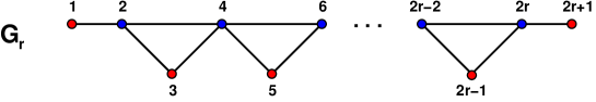
Figure 3. The graph $G_{r}$, with $2r+1$ vertices labeled $i=1,2,...,2r+1$.

Let $G_{r}$ be the graph of Figure 3. When $r=1$, $G_{1}$ is the chain with 3 vertices. To each vertex labeled $i$ in the graph, we assign the weight $y_{i}$.

Let $G$ be a graph with vertices labeled by the index set $I$.

Definition 3.7.

A hard particle configuration $C$ on $G$ is a subset of $I$ such that $i,j\in C$ only if there is no edge connecting vertices $i$ and $j$ in $G$.

Let ${\rm HP}(G)$ be the set of all hard particle configurations on $G$.

If we assign a weight $y_{i}$ to each vertex $i\in I$, the weight of a configuration $C$ is $w(C)=\prod_{i\in C}y_{i}$. The partition function of hard particles on $G$ is

(3.14) $$Z^{(G)}(\{y_{i}\})=\sum_{C\in{\rm HP}(G)}w(C).$$

If we limit the summation to the set of configurations fixed cardinality $j$, we have the $j$-particle partition function $Z_{j}^{(G)}$.

In the particular case $G=G_{r}$ of Figure 3, we have the partition function of $j$ hard particles on $G_{r}$, denoted by $Z_{j}^{(G_{r})}:=Z_{j}^{(G_{r})}(y_{1},...,y_{2r+1})$. These satisfy recursion relations, coming from the structure of $G_{r}$.

Theorem 3.8.

The partition functions $Z_{j}^{(G_{r})}$ satisfy the following recursion relations:

(3.15) $$Z_{j}^{(G_{r})}=Z_{j}^{(G_{r-1})}+y_{2r+1}Z_{j-1}^{(G_{r-1})}+y_{2r}Z_{j-1}^{(G_{r-2})}$$

Proof.

Depending on the occupation numbers of the last two vertices, three situations may occur:

1. Vertices $2r$ and $2r+1$ are both vacant. This is a configuration of $j$ hard particles on $G_{r-1}$, obtained by erasing these two vertices and their adjacent edges.

2. Vertex $2r+1$ is occupied, and hence the vertex $2r$ is empty. Such configurations are those of $j-1$ hard particles on $G_{r-1}$.

3. The vertex $2r$ is occupied, and hence vertices $2r+1$, $2r-1$ and $2r-2$ are empty. Such configurations are those of $j-1$ hard particles on $G_{r-2}$ obtained by erasing the vertices $2r-2,2r-1,2r,2r+1$ and their incident edges.

Each of these occupation states gives rise to one of the terms on the right hand side of the equation. ∎

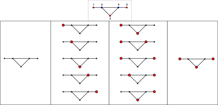
Figure 4. The configurations of hard particles on $G_{2}$, with, from left to right, $0$, $1$, $2$ or $3$ particles.

Example 3.9.

For $r=2$, the hard particle model on $G_{2}$ has the partition function

(3.16) $$Z^{(G_{2})}(y_{1},y_{2},y_{3},y_{4},y_{5})=1+(y_{1}+y_{2}+y_{3}+y_{4}+y_{5})+(y_{1}y_{3}+y_{1}y_{4}+y_{2}y_{5}+y_{3}y_{5}+y_{1}y_{5})+(y_{1}y_{3}y_{5}),$$

where the various terms correspond to the configurations depicted in Fig.4.

Theorem 3.10.

The $j$-th conserved quantity $c_{j}$ of the Q-system for $A_{r}$ is equal to the partition function $Z_{j}^{(G_{r})}(y_{1,n},...,y_{2r+1,n})$ for $j$ hard particles on the graph $G_{r}$, with vertex weights $y_{i}\equiv y_{i,n}$ defined in eq.(3.9), for $i=1,2,...,2r+1$, and for any choice of $n\in{\mathbb{Z}}$.

Proof.

The equations (3.11) and (3.15) are identical upon taking $y_{i}=y_{i,n}$. Moreover the initial conditions are also identical, as $Z_{0}^{(G_{r})}=C_{r+1,0,n}=1$. We deduce that $Z_{j}^{(G_{r})}=C_{r+1,j,n}=c_{j}$, independently of $n$. ∎

Corollary 3.11.

The conserved quantities $c_{j}$ can be expressed in terms ${\mathbf{x}}_{0}$ as the partition functions for $j$ hard particles on $G_{r}$, with vertex weights

(3.17) $$y_{2{\alpha}-1}={R_{{\alpha}-1,0}R_{{\alpha},1}\over R_{{\alpha},0}R_{{\alpha}-1,1}},\ \ 1\leq{\alpha}\leq r+1,\qquad y_{2{\alpha}}={R_{{\alpha}-1,0}R_{{\alpha}+1,1}\over R_{{\alpha},0}R_{{\alpha},1}},\ \ 1\leq{\alpha}\leq r.$$

Example 3.12.

In the case $G_{2}$ of Example 3.9, we have (with $y_{1}y_{3}y_{5}=1$): $c_{0}=c_{3}=1$, and

(3.18) $$c_{1} = {R_{2,0}\over R_{2,1}}+{R_{1,1}\over R_{1,0}}+{R_{1,0}R_{2,1}\over R_{2,0}R_{1,1}}+{R_{2,1}\over R_{1,0}R_{1,1}}+{R_{1,0}\over R_{2,0}R_{2,1}}$$

(3.19) $$c_{2} = {R_{1,0}\over R_{1,1}}+{R_{2,1}\over R_{2,0}}+{R_{2,0}R_{1,1}\over R_{1,0}R_{2,1}}+{R_{1,1}\over R_{2,0}R_{2,1}}+{R_{2,0}\over R_{1,0}R_{1,1}}$$

The two integrals of motion of the $A_{2}$ $Q$-system correspond to writing $c_{1}$ and $c_{2}$ with the substitutions $R_{{\alpha},i}\to R_{{\alpha},i+n-1}$, $i=0,1$, ${\alpha}=1,2$. These yield a system of recursion relations involving only indices $n$ and $n-1$, as opposed to the original $Q$-system, which involves the indices $n-1,n$ and $n+1$.

3.4. Generating functions

3.4.1. A generating function for $R_{1,n}$

It is useful to introduce generating functions. Define

(3.20) $$F_{1}^{(r)}(t)=\sum_{n\geq 0}R_{1,n}t^{n}$$

Theorem 3.13.

We have the relation

(3.21) $$F_{1}^{(r)}(t)={\sum_{j=0}^{r}(-1)^{j}d_{j}t^{j}\over\sum_{j=0}^{r+1}(-1)^{j}c_{j}t^{j}},\qquad d_{j}=\sum_{i=0}^{j}R_{1,j-i}(-1)^{j-i}c_{i}.$$

Proof.

Consider the product of series $\Big{(}\sum_{i=0}^{\infty}R_{1,i}t^{i}\Big{)}\Big{(}\sum_{j=0}^{r+1}(-1)^{j}c_{j}t^{j}\Big{)}$. Then all terms of order $r+1$ or higher in $t$ vanish, due to Theorem 2.8. We are left with the terms of order $0,1,...,r$, the term of order $j$ being exactly $(-1)^{j}d_{j}$. ∎

Example 3.14.

For $r=1$, we have $c_{1}={R_{1,1}\over R_{1,0}}+{1\over R_{1,0}R_{1,1}}+{R_{1,0}\over R_{1,1}}$ from Example 3.2, and $d_{0}=R_{1,0}$, $d_{1}=c_{1}R_{1,0}-R_{1,1}={R_{1,0}^{2}+1\over R_{1,1}}$, hence

(3.22) $$F_{1}^{(1)}(t)=R_{1,0}{1-\left({R_{1,0}\over R_{1,1}}+{1\over R_{1,0}R_{1,1}}\right)t\over 1-\left({R_{1,1}\over R_{1,0}}+{1\over R_{1,0}R_{1,1}}+{R_{1,0}\over R_{1,1}}\right)t+t^{2}}$$

3.4.2. Generating function and hard particles

Theorem 3.15.

(3.23) $$F_{1}^{(r)}(t)=R_{1,0}{Z^{(G_{r})}(0,-ty_{2},-ty_{3},...,-ty_{2r+1})\over Z^{(G_{r})}(-ty_{1},-ty_{2},-ty_{3},...,-ty_{2r+1})}$$

with $y_{i}$ as in (3.17).

Proof.

In the expression (3.21), the denominator is the partition function $Z^{(G_{r})}(-ty_{1},...,-ty_{2r+1})$, according to Corollary 3.11. The numerator of $F_{1}^{(r)}(t)/R_{1,0}$ is $\sum_{j=0}^{r}(-t)^{j}d_{j}/R_{1,0}$, where

$${d_{j}\over R_{1,0}}=\sum_{i=0}^{j}(-1)^{j-i}c_{i}{R_{1,j-i}\over R_{1,0}}.$$

We proceed as for the $c_{j}$. First, we relax the condition that $R_{r+1,n}=1$, hence work with the $r_{{\alpha},n}$, the solutions of (3.2). Define

(3.24) $$D_{{\alpha},m,n}=\sum_{i=0}^{m}(-1)^{m-i}C_{{\alpha},i,n}{r_{1,m-i}\over r_{1,0}}.$$

Then $d_{j}/r_{1,0}=D_{r+1,j,n}=D_{r+1,j,0}$, independently of $n$ when we impose the condition $r_{r+1,n}=1$, due to (3.13). Substituting the recursion relations (3.11) into this expression, we obtain an analogous recursion relation for $D_{{\alpha},m,0}$:

$$D_{{\alpha},m,0} = \sum_{i=0}^{m}(-1)^{m-i}{r_{1,m-i}\over r_{1,0}}(y_{2{\alpha}-1}C_{{\alpha}-1,i-1,0}+y_{2{\alpha}-2}C_{{\alpha}-2,i-1,0}+C_{{\alpha}-1,i,0})$$

$$= y_{2{\alpha}-1}D_{{\alpha}-1,m-1,0}+y_{2{\alpha}-2}D_{{\alpha}-2,m-1,0}+D_{{\alpha}-1,m,0},$$

with $C_{{\alpha},-1,0}=0$ and $y_{k}:=y_{k,0}$. The initial values of $D$ for ${\alpha}=1$ are $D_{1,0,0}=C_{1,0,0}=1$ and $D_{1,1,0}=C_{1,1,0}-y_{1}C_{1,0,0}=y_{2}+y_{3}$. Both coincide with the values of $C_{1,0,0}$ and $C_{1,1,0}$, respectively, when restricted to $y_{1}=0$. As the recursion relation for $D_{{\alpha},m,0}$ is identical to that for $C_{{\alpha},m,0}|_{y_{1}=0}$, we deduce that $D_{{\alpha},m,0}=C_{{\alpha},m,0}|_{y_{1}=0}$ for all ${\alpha},m$. This relation remains true after imposing the condition (3.12). Therefore

$$d_{j}=R_{1,0}\,D_{r+1,j,0}=R_{1,0}\,C_{r+1,j,0}(0,y_{2},...,y_{2r+1})$$

with the $y$’s as in Corollary 3.11. We deduce that the numerator of $F_{1}^{(r)}(t)/R_{1,0}$ is equal to the denominator of (3.21), restricted to the value $y_{1}=0$. ∎

3.4.3. Translational invariance

From the translational invariance property of Lemma 2.3, we may easily deduce an invariance property for the generating function $F_{1}^{(r)}(t)$. Let us first write $F_{1}^{(r)}(t)$ as an explicit expression $F_{1}^{(r)}(t)=\Phi((R_{{\alpha},0})_{{\alpha}=1}^{r};(R_{{\alpha},1})_{{\alpha}=1}^{r};t)$ involving only the initial data ${\mathbf{x}}_{0}$.

Theorem 3.16.

The generating function $\Phi$ satisfies the following translation property:

$$\Phi(R_{1,0},\ldots,R_{r,0};R_{1,1},\ldots,R_{r,1};t)=\sum_{n=0}^{k-1}R_{1,n}t^{n}+t^{k}\Phi(R_{1,k},\ldots,R_{r,k};R_{1,k+1},\ldots,R_{r,k+1};t)$$

for all $k\geq 0$.

Proof.

We write $F_{1}^{(r)}(t)=\sum_{n=0}^{k-1}R_{1,n}t^{n}+t^{k}\sum_{n\geq 0}R_{1,n+k}t^{n}$, and apply eq.(2.4) to all $R_{1,n+k}$ in the second term. ∎

4. Positivity: a heap interpretation

We now have an expression for the generating function of $R_{1,n}$ ($n\geq 0$) in terms of the ratio of two partition functions of hard particles. Positivity of the terms $R_{1,n}$, when expressed in terms of the fundamental cluster variables ${\mathbf{x}}_{0}$, follows from a theorem relating this ratio to the partition function of heaps. This interpretation also allows us to find an explicit formula for the generating function of cluster variables.

4.1. Heaps

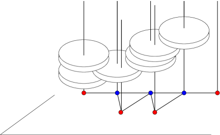
Figure 5. A heap on the graph $G_{3}$. Solid discs are piled up above each vertex of $G_{3}$. Diameters are such that only adjacent vertex discs may overlap.

Given a graph $G$, heaps on $G$ are defined as follows (see [24] and the beautiful expository article [18]).

The graph $G$ is represented in the $xy$ plane in ${\mathbb{R}}^{3}$, and we attach half-lines parallel to the positive $z$-axis, originating at each vertex of $G$. (See Figure 5). The vertices of $G$ are endowed with a partial ordering.

On each half-line above vertex $i$, we stack an arbitrary number of discs of radius $R_{i}$ and thickness $a$, with a hole at their center, so that they can freely slide along the half-lines (gravity points in the negative $z$-direction). The disc radii $R_{i}$ are such that the distance between any pair of adjacent vertices $i,j$ of $G$ is $<R_{i}+R_{j}$, while the distance between any pair of non-adjacent vertices $i,j$ is $>R_{i}+R_{j}$. Thus, the order in which the various discs are stacked matters only on neighboring half-lines (i.e. with connected projections on $G$), but not on distant ones.

For a given stack of discs, its foreground is the set of discs that touch the $xy$-plane. A stack is said to be admissible if it is empty or if its foreground is reduced to one disc, positioned at a vertex of smallest order. (Such configurations are also called “pyramids” in the heap jargon [24]) We will call such admissible stacks of discs heaps on $G$.

To each heap $h$ on $G$, we associate a weight $W(h)=\prod_{d\in h}W(d)$, where the product extends over all discs $d$ of the heap, and where the weight $W(d)=z_{i}$ if $d$ is stacked above vertex $i$. The partition function for heaps on $G$ is

(4.1) $$\Phi^{(G)}(\{z_{i}\})=\sum_{h\ {\rm heap}\ {\rm on}\ G}W(h)$$

Theorem 4.1.

(4.2) $$\Phi^{(G)}(\{z_{i}\})={Z^{(G)}(0,-z_{2},-z_{3},\ldots)\over Z^{(G)}(-z_{1},-z_{2},-z_{3},\ldots)}$$

Proof.

This follows from the general theory of heaps [24] [18]. We write

(4.3) $$\qquad\Phi^{(G)}(\{z_{i}\})\ Z^{(G)}(-z_{1},-z_{2},-z_{3},\ldots)=\sum_{(h,c)}W(h)\,w(c)=Z^{(G)}(0,-z_{2},-z_{3},\ldots)=\sum_{c^{\prime}\ {\rm with}\atop{\rm vertex}\ 1\ {\rm empty}}w(c^{\prime})$$

where the sums extend over pairs $(h,c)$ made of a heap $h$ and a configuration $c$ of hard particles on $G$, and configurations $c^{\prime}$ of hard particles on $G$ such that the vertex 1 remains unoccupied.

We define an involution $\varphi$ between pairs $(h,c)$ which reverses the sign of $W(h)\,w(c)$. Let $c\circ h$ be the heap obtained by replacing the particles of $c$ by discs, and by adding those discs on top of $h$. We define the background of any heap $h$ to be the foreground of the heap obtained by flipping the configuration upside-down. In particular, the background of $c\circ h$ contains $c$. Let $d$ be the disc in the background of $c\circ h$ that has the smallest vertex index $i$. Then if $i$ is occupied in $c$, we form $c^{\prime}$ by removing the particle at $i$, and $h^{\prime}$ by adding a disc on top of the $i$ vertex. If $i$ is unoccupied in $c$, then we form $c^{\prime}$ by adding a particle at $i$, and $h^{\prime}$ by removing the top disc at $i$. Finally if $h$ is empty and the vertex $1$ is unoccupied in $c$, then we leave the pair unchanged. These rules define an involution $\varphi(h,c)=(h^{\prime},c^{\prime})$. By construction, we have $W(h)\,w(c)=-W(h^{\prime})\,w(c^{\prime})$, if $(h^{\prime},c^{\prime})\neq(h,c)$. Hence the distinct pairs $((h,c),(h^{\prime},c^{\prime}))$ image of one-another under $\varphi$ contribute zero to the sum on the l.h.s. of eq. (4.3), and we are left only with the contribution of the fixed points of the involution. The latter correspond to the situation where $h=\emptyset$ and $c$ has no particle at the vertex $1$, producing the r.h.s. of (4.3). ∎

4.2. Positivity from heaps

Applying Theorem 4.1 to the case of $G=G_{r}$, and comparing the expressions (3.23) and (4.2), we arrive at the main theorem of this section, which allows to interpret the $R_{1,n}$ as partition functions for heaps.

Theorem 4.2.

The solution $R_{1,n}$ to the Q-system for $n\geq 0$ is, up to a multiplicative factor $R_{1,0}$, the partition function for configurations of heaps of $n$ discs on $G_{r}$ with weights $z_{i}=ty_{i}$, with $y_{i}$ as in (3.17).

Proof.

Using Theorem 3.15, we may rewrite $F_{1}^{(r)}(t)/R_{1,0}$ exactly in the form of the r.h.s. of (4.2), with $G=G_{r}$ and the weights $z_{i}=ty_{i}$. We deduce that $F_{1}^{(r)}(t)/R_{1,0}$ is the generating function for heaps on $G_{r}$ with weight $ty_{i}$ per disc above the vertex $i$. The coefficient of $t^{n}$ in the corresponding series corresponds to heap configurations with exactly $n$ discs. ∎

Corollary 4.3.

For all $n\in{\mathbb{Z}}$, $R_{1,n}$ is a positive Laurent polynomial of the initial seed ${\mathbf{x}}_{0}$.

Proof.

By Theorem 4.2, $R_{1,n}/R_{1,0}$ for $n\geq 0$ is a sum over heap configurations, each contributing a weight made of a product of $y_{i}$’s. The resulting sum is therefore a manifestly positive polynomial of the $y_{i}$’s, themselves products of ratios of initial data. For $n<0$, the result follows by applying the Lemma 2.1. ∎

4.3. Continued fraction expressions for generating functions

The heap interpretation allows us to write an explicit expression for $F_{1}^{(r)}(t)$ as a rational function of $t$.

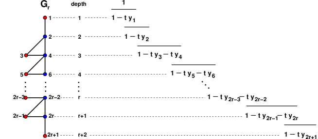
Figure 6. The graph $G_{r}$, arranged into a hierarchical structure. The depth of the vertices is indicated on the center, and the corresponding terms of the continued fraction for the generating function $F_{1}^{(r)}(t)$ are displayed on the right.

Theorem 4.4.

(4.4) $$F_{1}^{(r)}(t)={R_{1,0}\over 1-t{y_{1}\over 1-t{y_{2}\over 1-ty_{3}-t{y_{4}\over 1-ty_{5}-t{y_{6}\over\ddots{{}\over 1-ty_{2r+1}}}}}}}$$

where $y_{i}$ are defined in (3.17).

Proof.

Define a partial ordering on the vertices of $G_{r}$ by their geodesic distance from vertex 1. Any nonempty heap on $G_{r}$ is constructed by repeating the following two steps:

1. Stack one disc above vertex $1$.

2. Construct a heap on the graph $G_{r}^{\prime}=G_{r}\setminus\{1\}$ (the graph $G_{r}$ without the vertex $1$ and its incident edges).

Let $c(t)$ be the generating function for heaps on $G_{r}^{\prime}$, then clearly ${F_{1}^{(r)}(t)/R_{1,0}}={1/(1-t{y_{1}c(t)})}.$ Similarly, $c(t)$ is found via a similar construction of heaps on $G_{r}^{\prime}$. Clearly, $c(t)=1/(1-ty_{2}d(t))$, where $d(t)$ is the generating function for heaps on the graph $G_{r}^{\prime\prime}=G_{r}^{\prime}\setminus\{2\}$.

To find $d(t)$, we note that $G_{r}^{\prime\prime}$ has two minimal vertices, but they are connected, so that a heap on $G_{r}^{\prime\prime}$ may have as its foreground either node $3$ or node $4$ but not both. Thus, $d(t)={1/(1-ty_{3}-ty_{4}e(t))}$, where $e(t)$ is the generating function for heaps on $G_{r}^{\prime\prime}\setminus\{3,4\}$. This procedure is iterated (see Figure 6), resulting in Equation (4.4). ∎

When expanded as a power series in $t$, (4.4) has manifestly positive coefficients which are Laurent polynomials in the $y_{i}$’s.

4.4. Continued fraction rearrangements

One can rewrite the continued fraction expression for $F_{1}^{(r)}(t)$ in various ways using two simple Lemmas:

Lemma 4.5.

For all $a$, $b$ there is an identity of power series of $t$:

(4.5) $${1\over 1-t{a\over 1-tb}}=1+t{a\over 1-ta-tb}.$$

and

Lemma 4.6.

For all $a$, $b$, $c$, $d$ such that $c\neq 0$ and $a+b\neq 0$,

(4.6) $$a+{b\over 1-t{c\over 1-td}}={a^{\prime}\over 1-t{b^{\prime}\over 1-tc^{\prime}-td}}$$

where

(4.7) $$a^{\prime}=a+b,\quad b^{\prime}={bc\over a+b},\quad c^{\prime}={ac\over a+b},\quad a={a^{\prime}c^{\prime}\over b^{\prime}+c^{\prime}},\quad b={a^{\prime}b^{\prime}\over b^{\prime}+c^{\prime}},\quad c=b^{\prime}+c^{\prime}$$

For example, applying Lemma 4.5 to the expression (4.4) with $a=y_{1}$ and $b=y_{2}/(1-ty_{3}\cdots)$, we have

(4.8) $$F_{1}^{(r)}(t)=R_{1,0}\Big{(}1+t{y_{1}\over 1-ty_{1}-{ty_{2}\over 1-ty_{3}-{ty_{4}\over\ddots{{}\over 1-ty_{2r-1}-{ty_{2r}\over 1-ty_{2r+1}}}}}}\quad\Big{)}$$

where $y_{i}$ are defined in (3.17).

Example 4.7.

For $r=1$, we have

(4.9) $$F_{1}^{(1)}(t)=R_{1,0}\Big{(}1+{t{R_{1,1}\over R_{1,0}}\over 1-t{{R_{1,1}\over R_{1,0}}-{{t\over R_{1,0}R_{1,1}}\over 1-t{R_{1,0}\over R_{1,1}}}}}\quad\Big{)}={R_{1,0}\over 1-t{{R_{1,1}\over R_{1,0}}\over 1-t{{1\over R_{1,0}R_{1,1}}\over 1-t{R_{1,0}\over R_{1,1}}}}}$$

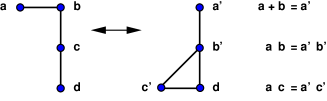
Figure 7. The local transformation of Lemma 4.6.

Figure 7 is a graphical interpretation of Lemma 4.6. It shows that the generating function of heaps on $G$ can be rewritten as a generating function for heaps on $G^{\prime}$ with new weights. Note that $a,b,c,d$ and the associated nodes might stand for composite generating functions and the associated subgraphs.

Starting from the initial seed ${\mathbf{x}}_{0}$ and its associated graph $G_{r}$, repeated application of Lemmas 4.5 and 4.6 on the expression (4.8) produces new expressions for $F_{1}^{(r)}(t)$ with manifestly positive series expansions in $t$.

Writing the expression in (4.8) as $F_{1}^{(r)}(t)\equiv F_{{\mathbf{M}}_{0}}({\mathbf{x}}_{0};t)$, let ${\mathbf{x}}_{M}$ be another seed in the fundamental domain. Then we claim that there is a sequence $\Lambda$ of applications Lemmas 4.5 and 4.6, such that $\Lambda(F_{1}^{(r)}(t))=F_{\mathbf{M}}({\mathbf{x}}_{\mathbf{M}})$. It turns out that we can generate in this way all the mutations of ${\mathbf{x}}_{0}$ within the fundamental domain ${\mathcal{F}}_{r}$. The proof of this statement appears in Section 6. Here, we illustrate this result with the example of $A_{2}$. The example of $A_{3}$ is given in Appendix A.

Example 4.8.

Consider the case of $A_{2}$. We present all the rearrangements of $F_{1}^{(2)}(t)$ which correspond to mutations of the weights within the fundamental domain.

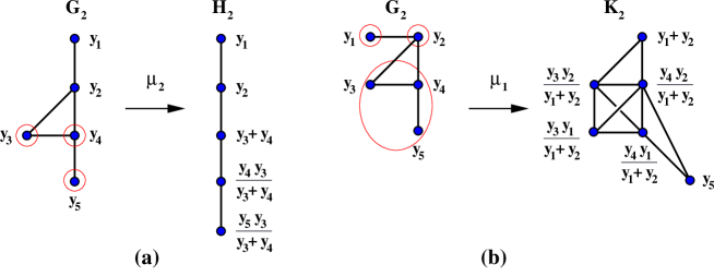
Figure 8. The graph heap formulation of the application of Lemma 4.6 on the generating function $F_{1}^{(r)}(t)/R_{1,0}$ (a), and on the generating function $\Phi(t)$ such that $F_{1}^{(r)}(t)=R_{1,0}+tR_{1,1}\Phi(t)$ (b). The circled vertices correspond to $a,b,c$ in the Lemma 4.6.

1. $F_{{\mathbf{M}}_{0}}({\mathbf{x}}_{0})$ with ${\mathbf{x}}_{0}=(R_{1,0},R_{2,0};R_{1,1}R_{2,1})$: Equation 4.8 is

   (4.10) $$F_{1}^{(2)}(t)=R_{1,0}+t{R_{1,1}\over 1-ty_{1}-{ty_{2}\over 1-ty_{3}-{ty_{4}\over 1-ty_{5}}}}$$

   with

   (4.11) $$y_{1}={R_{1,1}\over R_{1,0}},\ \ y_{2}={R_{2,1}\over R_{1,0}R_{1,1}},\ \ y_{3}={R_{1,0}R_{2,1}\over R_{2,0}R_{1,1}},\ \ y_{4}={R_{1,0}\over R_{2,0}R_{2,1}},\ \ y_{5}={R_{2,0}\over R_{2,1}}.$$

2. $F_{\mu_{2}({\mathbf{M}}_{0})}(\mu_{2}({\mathbf{x}}_{0}))$, where $\mu_{2}({\mathbf{x}}_{0})=(R_{1,0},R_{2,2};R_{1,1}R_{2,1})$: Use Lemma 4.6 with $a=y_{3}$, $b=y_{4}$, $c=y_{5}$ and $d=0$. Then

   (4.12) $$F_{1}^{(2)}(t)=R_{1,0}+t{R_{1,1}\over 1-tx_{1}-{tx_{2}\over 1-{tx_{3}\over 1-{tx_{4}\over 1-tx_{5}}}}}={R_{1,0}\over 1-{tx_{1}\over 1-{tx_{2}\over 1-{tx_{3}\over 1-{tx_{4}\over 1-tx_{5}}}}}}$$

   where the second expression follows from application of Lemma 4.5 with $a=x_{1}$. Here

   $$x_{1} = y_{1}={R_{1,1}\over R_{1,0}},\quad x_{2}=y_{2}={R_{2,1}\over R_{1,0}R_{1,1}}$$

   $$x_{3} = a^{\prime}=a+b=y_{3}+y_{4}={R_{1,0}(R_{2,1}^{2}+R_{1,1})\over R_{2,1}R_{1,1}R_{2,0}}={R_{1,0}R_{2,2}\over R_{2,1}R_{1,1}}$$

   $$x_{4} = b^{\prime}={bc\over a^{\prime}}={y_{4}y_{5}\over y_{3}+y_{4}}={R_{1,0}\over R_{2,1}^{2}a^{\prime}}={R_{1,1}\over R_{2,1}R_{2,2}}$$

   (4.13) $$x_{5} = c^{\prime}={ac\over a^{\prime}}={y_{3}y_{5}\over y_{3}+y_{4}}={R_{1,0}\over R_{1,1}a^{\prime}}={R_{2,1}\over R_{2,2}}.$$

   by use of the $Q$-system. This is an expression for the generating function in terms of $(R_{1,0},R_{2,2};R_{1,1}R_{2,1})=\mu_{2}({\mathbf{x}}_{0})$. It has a manifestly positive series expansion in $t$.

   Figure 8 (a) illustrates this transformation. The generating function is interpreted in terms of that for heaps on $H_{2}$:

   $$F_{1}^{(2)}(t)=R_{1,0}{Z^{(H_{2})}(0,-tx_{2},-tx_{3},-tx_{4},-tx_{5})\over Z^{(H_{2})}(-tx_{1},-tx_{2},-tx_{3},-tx_{4},-tx_{5})}$$

3. $F_{\mu_{1}({\mathbf{M}}_{0})}(\mu_{1}({\mathbf{m}}_{0}))$, where $\mu_{1}({\mathbf{x}}_{0})=(R_{1,2},R_{2,0};R_{1,1}R_{2,1})$: Use Lemma 4.6 on (4.10), with $a=y_{1}$, $b=y_{2}$, $c=y_{3}+y_{4}/(1-ty_{5})={R_{1,0}\over R_{2,0}R_{2,1}R_{1,1}}\Big{(}R_{2,1}^{2}+R_{1,1}/(1-t{R_{2,0}\over R_{2,1}})\Big{)}$, and $d=0$ (see Fig.8 (b)):

   (4.14) $$F_{1}^{(2)}(t)=R_{1,0}+t{R_{1,1}\over 1-{tz_{1}\over 1-t{z_{2}+{z_{6}\over 1-tz_{5}}\over 1-tz_{3}-t{z_{4}\over 1-tz_{5}}}}}$$

   with

   $$z_{1} = a^{\prime}=a+b=y_{1}+y_{2}={R_{1,1}^{2}+R_{2,1}\over R_{1,0}R_{1,1}}={R_{1,2}\over R_{1,1}}$$

   $$z_{2}+{z_{6}\over 1-tz_{5}} = b^{\prime}={bc\over a+b}=y_{2}\Big{(}y_{3}+{y_{4}\over 1-ty_{5}}\Big{)}={1\over R_{2,0}R_{1,2}R_{1,1}}\left(R_{2,1}^{2}+{R_{1,1}\over 1-t{R_{2,0}\over R_{2,1}}}\right)$$

   (4.15) $$\qquad z_{3}+{z_{4}\over 1-tz_{5}} = c^{\prime}={ac\over a+b}=y_{1}\Big{(}y_{3}+{y_{4}\over 1-ty_{5}}\Big{)}={R_{1,1}\over R_{2,0}R_{2,1}R_{1,2}}\left(R_{2,1}^{2}+{R_{1,1}\over 1-t{R_{2,0}\over R_{2,1}}}\right).$$

   where we have used the $Q$-system. This yields positivity of all $R_{1,n}$ in terms of $(R_{1,2},R_{2,0};R_{1,1}R_{2,1})=\mu_{1}({\mathbf{x}}_{0})$, by noting that $R_{1,0}=(R_{1,1}^{2}+R_{2,1})/R_{1,2}$.

   Figure 8 (b) illustrates this transformation. (4.14) may be rewritten in terms of the generating function of heaps on $K_{2}$ as:

   $$F_{1}^{(2)}(t)=R_{1,0}+R_{1,1}t{Z^{(K_{2})}(0,-tz_{2},-tz_{3},-tz_{4},-tz_{5},-tz_{6})\over Z^{(K_{2})}(-tz_{1},-tz_{2},-tz_{3},-tz_{4},-tz_{5},-tz_{6})}.$$

   Note that the graph $K_{2}$ has one more node than $G_{2}$ and $H_{2}$, but the weights depend on the same number ($4$) of free parameters, since $z_{1}z_{3}z_{5}=1$, and $z_{2}z_{4}=z_{3}z_{6}$.

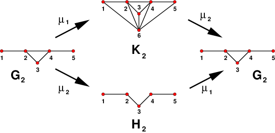
Figure 9. The graphs encoding the $R_{1,n}$’s for the case $A_{2}$, and the corresponding mutations of cluster variables.

The rearranged expressions for $F_{1}^{(2)}(t)$ considered above have been related to mutations of cluster variables in the fundamental domain ${\mathcal{F}}_{2}$, as well as to configurations of heaps on particular graphs, see Figure 9.

5. Path generating functions

In order to prove the claim of the last section, it is simpler to work with a path interpretation. There exist certain bijections between the partition function of heaps on a graph $G$, and the partition function of paths on an associated weighted rooted graph $\widetilde{G}$. Such bijections are standard in the theory of heaps [24].

We will establish this bijection in the case of $G_{r}$. Then, we construct bijections between Motzkin paths representing cluster variables in the fundamental domain, and weighted graphs, on which the path partition function gives the generating function $F_{1}^{(r)}(t)$, in terms of the new cluster variables. For completeness, we give the bijection with the related graphs for heaps at the end of this section.

5.1. From heaps on $G_{r}$ to paths on $\widetilde{G}_{r}$

We start with the graph $G_{r}$ defined in Figure 3.

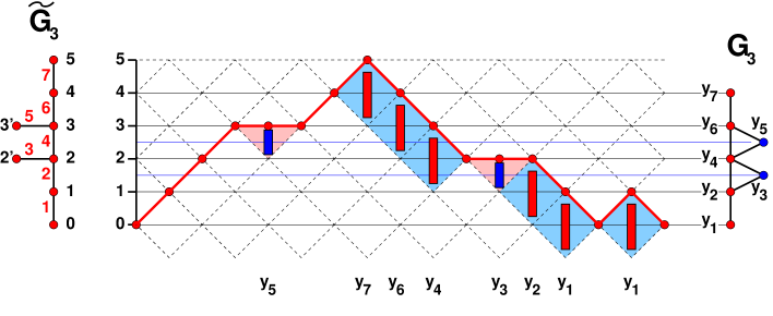
Figure 10. A heap on $G_{3}$ with 8 discs, and the corresponding lattice path of length $16$. The heap has small discs above vertices $3$ and $5$ of $G_{3}$, and large discs above the other vertices. The large discs are in bijection with the descending steps, and the small discs are in bijection with the horizontal steps. This path has weight $y_{1}^{2}y_{2}y_{3}y_{4}y_{5}y_{6}y_{7}$. On the left is the path graph ${\tilde{G}}_{3}$, with labeled vertices (in black) and labeled edges (in gray).

Definition 5.1.

The graph ${\widetilde{G}}_{r}$ is a vertical chain of $r+3$ vertices labeled $0,1,2,...,r+2$, with $r+2$ vertical edges $(i,i+1)$ ($0\leq i\leq r+1$), together with $r-1$ vertices $2^{\prime},3^{\prime},...,r^{\prime}$ and $r-1$ horizontal edges $(i,i^{\prime})$ ($2\leq i\leq r$). It is rooted at its bottom vertex $0$. (See the left of Fig.10 for the $r=3$ example.)

The graph ${\widetilde{G}}_{r}$ is “dual” to $G_{r}$, in the sense that its edges are in bijection with the vertices of $G_{r}$. We may denote the edges by the same labels, $i=1,2,...,2r+1$.

Definition 5.2.

The weights of $\widetilde{G}_{r}$ are defined as follows. There is a weight $y_{i}$ for each step along the edge $i$ which goes towards the root vertex $0$, and a weight $1$ to all others. That is, the step $i^{\prime}\to i$ has weight $y_{2i-1}$, the step $i\to i-1$ has weight $y_{2i}$ if $1<i<r+1$, step $1\to 0$ has weight $y_{1}$, and step $r+2\to r+1$ has weight $y_{2r+1}$.

Paths along $\widetilde{G}_{r}$, from the root to the root, also referred to as $\widetilde{G}_{r}$-paths below, can be represented on a two-dimensional lattice as follows. Paths of length $2n$ start at the point $(0,0)$, end at the point $(2n,0)$, and cannot go below 0 or above $r+2$. They may contain steps of the type $(i,j)\to(i+1,j\pm 1)$ (if $j\pm 1$ is in the range $0,...,r+2$), and steps $(i,j)\to(i+2,j)$ ($2\leq j\leq r$).

Theorem 5.3.

The heaps on $G_{r}$ with $n$ discs are in bijection with the $\widetilde{G}_{r}$-paths of length $2n$, and their partition functions are equal, with weights as in Definition 5.2.

Proof.

Given a heap on the graph $G_{r}$, we associate a large disc to each vertex along the “backbone” $\{1,2,4,...,2r-2,2r,2r+1\}$. We associate a small disc to the other vertices, $\{3,5,...,2r-1\}$. The overlap between discs is given by the graph $G_{r}$, namely two discs overlap if and only if the corresponding vertices of $G_{r}$ are connected via an edge. These discs are represented by bars in the plane in Figure 10.

We draw the bars on the faces of a tilted square lattice, in such a way that they are in bijection with the descending (for a large disc) or horizontal (for a small disc) steps of the two-dimensional representation of a $\widetilde{G}_{r}$-path. In this picture, the descending steps of the path are the north-east edges of the square faces in which the large discs sit, while the horizontal steps are the horizontal diagonals of the square faces in which the small discs sit.

There is a unique way of placing the discs with this constraint. We decompose the heap into successive shells. Each shell has faces containing the discs placed from the bottom to the top and from left to right, the spaces in-between being covered with only up steps. In this way, each large disc corresponds to a descending step and each small one to a double horizontal step of the path. The correspondence of weights is clear: descending steps receive the weights of the corresponding large discs, while the horizontal steps receive the weights of the corresponding small discs.

Conversely, given a $\widetilde{G}_{r}$-path, we associate bijectively a large disc to each descending step and a small disc to each horizontal step. The resulting configuration is a heap over $G_{r}$, as the path always ends with a descending step corresponding to a disc over vertex 1 of $G_{r}$. ∎

Corollary 5.4.

For $n\geq 0$, the solution $R_{1,n}$ of (1.4), expressed in terms of the variables ${\mathbf{x}}_{0}$, is $R_{1,0}$ times the partition function of $\widetilde{G}_{r}$-paths of length $2n$, with weights as in Definition 5.2.

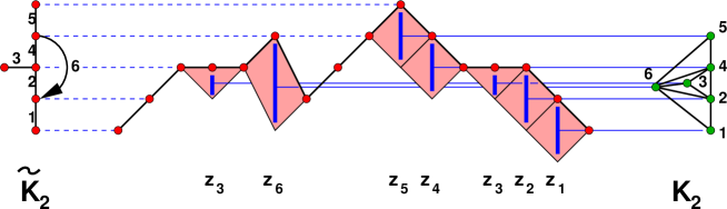
Figure 11. The bijection between heaps on $K_{2}$ and paths on the “dual” graph ${\tilde{K}}_{2}$. The discs of the heap give rise to polygons, whose top right edges are exactly the descending steps of the path. We have indicated the weights $z_{i}$ of the various discs, that are transferred to the descending steps of the path. We have indicated the vertex labels on $K_{2}$, and the corresponding dual edge labels on ${\tilde{K}}_{2}$.

The partition function for heaps $F_{1}^{(r)}$ on other the graphs corresponding to fraction rearrangements can also be written in terms of paths on graphs. For example, it is easy to see that the path graph $\widetilde{H}_{r}$ corresponding to the heap graph $H_{r}$ (the chain with $2r+1$ vertices) is a vertical chain with $2r+2$ vertices, with edge $(i,i+1)$ of $\widetilde{H}_{r}$ corresponding to vertex $i+1$ in $H_{r}$. The edge weights for descending edges are the same as the corresponding vertex. Ascending edges have weight 1.

Example 5.5.

Consider the case of $A_{2}$ (see Fig.9). We have a path formulation of the partition function in terms of paths on $\widetilde{G}_{2}$ as a function of ${\mathbf{x}}_{0}$. Paths on the graph $\widetilde{H}_{2}$ correspond to the generating function in terms of $\mu_{2}({\mathbf{x}}_{0})$. The path formulation for the cluster variable $\mu_{1}({\mathbf{x}}_{0})$, corresponding to heaps on $K_{2}$, is the partition function for graphs on the graph $\widetilde{K}_{2}$ in Figure 11. Note that the edge labeled 6 is an oriented edge (with weight $z_{6}$).

In general, it is quite complicated to work out the direct bijection between $G$ and $\widetilde{G}$. Instead, we introduce a bijection between Motzkin paths in the fundamental domain and path graphs, and a bijection between the same Motzkin paths and heap graphs. This establishes an identification between path and heap partition functions in the cases of interest.

5.2. Motzkin paths and path graphs

5.2.1. The graphs $\Gamma_{\mathbf{M}}$

For any Motzkin path ${\mathbf{M}}$ in the fundamental domain, we associate a graph $\Gamma_{\mathbf{M}}$ by (1) decomposing ${\mathbf{M}}$ into “strictly descending” pieces; (2) associating a subgraph to each descending piece and (3) gluing the subgraphs.

1. Decomposition of ${\mathbf{M}}$: Each path ${\mathbf{M}}$, consists of strictly descending pieces ${\mathbf{m}}_{1},{\mathbf{m}}_{2},...,{\mathbf{m}}_{p}$, where ${\mathbf{m}}_{i}=\{(x,y),(x-1,y+1),...\}$. (We consider a single vertex to be a descending piece). These are separated by $p-1$ ascending steps of type (i) the step (1,1) in the plane, or (ii) the step (0,1) in the plane.

2. Graphs for ${\mathbf{m}}_{i}$: For each strictly descending piece ${\mathbf{m}}$ with $k$ vertices, we define a $\Gamma(k):=\Gamma_{{\mathbf{m}}}$ as follows. When $k=1$, ${\mathbf{m}}$ is a single vertex, and $\Gamma(1)$ is a chain of four vertices, as shown in the top left of Figure 12.

   

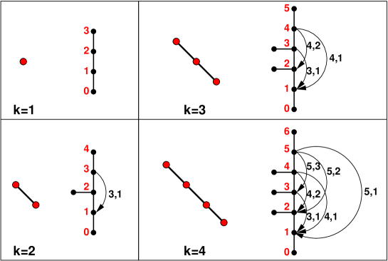
   Figure 12. The graphs $\Gamma(k)$ corresponding to strictly descending Motzkin paths with $k=1,2,3,4$ vertices. We have indicated the extra edge labels (in black) and the vertex labels (gray) along the vertical chain for the case when $i=j=0$.

   When ${\mathbf{m}}$ contains $k\geq 2$ vertices, the graph $\Gamma_{\mathbf{m}}=\Gamma(k)$ consists of a “skeleton” $\widetilde{G}_{k}$, plus extra oriented edges $j\to i$ if $j-i>1$, $j<k+2$ and $i>0$. There is a total of $k(k-1)/2$ extra oriented edges in $\Gamma(k)$, which we label by the vertices they connect. See Figure 12.

   Each $\Gamma(k)$ has four distinguished vertices denoted by $(t,t^{\prime},b^{\prime},b)=(k+2,k+1,1,0)$.

   

   Figure 13. The graphs $\Gamma_{{\mathbf{m}}_{i-1}}$ and $\Gamma_{{\mathbf{m}}_{i}}$ are glued together according to whether the pieces ${\mathbf{m}}_{i-1}$ and ${\mathbf{m}}_{i}$ are separated by a step of type (i) or (ii).

3. Gluing the subgraphs: Ascending steps of ${\mathbf{M}}$ are of type (i) $(1,1)$ or (ii) $(0,1)$. The graph $\Gamma_{\mathbf{M}}$ is obtained by gluing the graphs $\Gamma_{{\mathbf{m}}_{i}}$, $i=1,2,...,p$ as follows. Denote the edge $(t^{\prime},t)$ of $\Gamma_{{\mathbf{m}}_{i}}$ by $(t^{\prime}_{i},{\rm t}_{i})$, and so forth. We then make the following identifications of vertices and edges (See Figure 13):

   • Type (i): Identify ${\rm t}_{i-1}$ with $b^{\prime}_{i}$ and $t^{\prime}_{i-1}$ with $b_{i}$. The common edge is represented vertically.

   • Type (ii): Identify ${\rm t}_{i-1}$ with $b_{i}$ and $t^{\prime}_{i-1}$ with $b^{\prime}_{i}$. The common edge is represented horizontally.

   We denote this gluing procedure by the symbol “$|$”. Thus,

   (5.1) $$\Gamma_{\mathbf{M}}=\Gamma_{{\mathbf{m}}_{1}}|\Gamma_{{\mathbf{m}}_{2}}|\cdots|\Gamma_{{\mathbf{m}}_{k}}.$$

   Finally, all vertices are renumbered sequentially from bottom to top.

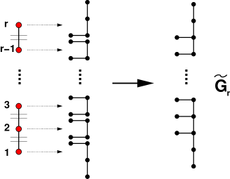
Figure 14. The graph $\Gamma_{{\mathbf{M}}_{0}}$ corresponding to the vertical Motzkin path ${\mathbf{M}}_{0}$ with $r$ vertices. The path is decomposed into $k$ isolated vertices, each corresponding to a chain of type $\Gamma(1)$, glued as indicated. The resulting graph is the tree ${\tilde{G}}_{r}$.

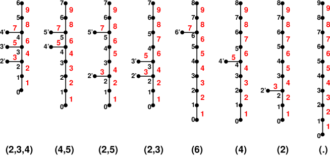
Figure 15. The 8 trees $T_{2r+2}(i_{1},i_{2},...,i_{s})$ for $r=4$. We have indicated the values of the $i$’s under each tree, and the labeling of the edges (gray) and vertices (black).

Example 5.6.

Consider the case of an ascending Motzkin path containing steps of type (i) and (ii) only. It decomposes into $r$ isolated vertices, corresponding to $\Gamma_{{\mathbf{m}}_{i}}=\Gamma(1).$ For the path ${\mathbf{M}}_{0}$, with steps only of type (ii), the result is $\Gamma_{{\mathbf{M}}_{0}}=\widetilde{G}_{r}$ (see Fig.14).

More generally, $\Gamma_{\mathbf{M}}$ is obtained by gluing $r$ chains ${\Gamma}(1)$ vertically or horizontally.

The path ${\mathbf{M}}$ is composed of $p$ vertical chains of lengths $l_{1},...,l_{p}\geq 1$, with steps of type (ii) only with $\sum_{i=1}^{p}l_{i}=r$. These are separated by $p-1$ steps of type (i). Each vertical chain corresponds to a graph $\widetilde{G}_{l_{i}}$, which are glued according to rule (i). This results in a tree which has a vertical chain of length $2+\sum_{i}(l_{i}+1)$, and consecutive sequences of $l_{i}-1$ horizontal edges, separated by pairs of vertices. The top two and bottom two vertices have no horizontal edge attached. (see Fig.15 for $r=4$).

The vertices $i_{j}$ to which the horizontal edges are attached $1<i_{1}<i_{2}<\cdots<i_{s}<2r-s$ where $s=r-p$, have the property that $i_{1}-1$ is odd, and $i_{j+1}-i_{j}$ is odd for all $j<s$. In fact,

$$\{i_{1},i_{2},\ldots,i_{s}\}=\{0,1,2,\ldots,2r-s+1\}\setminus\cup_{0\leq j\leq p}\{j+\sum_{i=1}^{j}l_{i},j+1+\sum_{i=1}^{j}l_{i}\}.$$

Definition 5.7.

The trees obtained in the previous example are denoted by $T_{2r+2}(i_{1},i_{2},...,i_{s})$.

The $2r+1$ edges of such trees are ordered from bottom to top and labeled $1,2,..,2r+1$, including the horizontal edges, which have labels $i_{1}+1,i_{2}+2,...,i_{s}+s$.

Noting that the sequence $j_{a}=(i_{a}+a-1)/2$ satisfies $1\leq j_{1}<j_{2}<\cdots<j_{s}\leq r-1$ without further constraint, we see that there are exactly $r-1\choose s$ such trees for $r$ and $s$ fixed, hence a total of $2^{r-1}$ when we sum over $s=0,1,2,...,r-1$. Note that when $s=0$, $T_{2r+2}()={\tilde{H}}_{r}$, “dual” of the chain of $2r+1$ vertices $H_{r}$ introduced in Section 5.1.

This example is important, as it illustrates all $2^{r-1}$ possible skeleton trees any $\Gamma_{\mathbf{M}}$ in the fundamental domain can have:

Definition 5.8.

The skeleton tree associated to ${\mathbf{M}}$ is the tree $\Gamma_{{\mathbf{M}}^{\prime}}$, where ${\mathbf{M}}^{\prime}$ is obtained from ${\mathbf{M}}$ by replacing all the steps $(-1,1)$ by vertical steps $(0,1)$. In other words, $\Gamma_{{\mathbf{M}}^{\prime}}$ is obtained from $\Gamma_{\mathbf{M}}$ by removing all its extra down-pointing edges.

5.2.2. Weights on $\Gamma_{\mathbf{M}}$

We will compute the partition function of paths on $\Gamma_{\mathbf{M}}$, for which purpose, we assign a weight to each oriented edge of $\Gamma_{\mathbf{M}}$. An unoriented edge, in this context, is considered to be a pair of edges oriented in opposite directions. The edge $(v,v^{\prime})$ is considered to be an ascending edge if the distance of $v^{\prime}$ from the vertex 0 is greater than that of $v$. Otherwise, it is a descending edge. We assign weight $1$ to all ascending edges, and weight $y_{e}({\mathbf{M}})$ to each descending edge $e$.

Edges are labeled as follows. Given $\Gamma_{{\mathbf{M}}}$, consider the skeleton tree $\Gamma_{{\mathbf{M}}^{\prime}}=T_{2r+2}(i_{1},i_{2},...,i_{s})$ of Definition 5.7. Its edges have labels $1,2,...,2r+1$, which we retain for the graph $\Gamma_{\mathbf{M}}$, and we assign to the descending skeleton edge $i$ the weights $y_{i}$ (these are independent variables, not necessarily related to the weights encountered earlier).

The extra descending edges of $\Gamma_{\mathbf{M}}$ are labeled by the pairs $(i,j)$ of vertices they connect, with $1<j+1<i\leq 2r-s$ (see Figure 12). The weights $y_{i,j}$ corresponding to down-pointing edges $e=(i,j)$ with $i-j>1$ can be expressed in terms of the skeleton weights. In view of the gluing procedure, we restrict our attention to strictly descending Motzkin paths ${\mathbf{m}}$ with $k$ vertices (see Fig.12). There are $k(k-1)/2$ descending edges of type $(i\to j)$, $2\leq j+1<i\leq k+1$. Then

(5.2) $$(y_{2j},y_{j+2,j},...,y_{k+1,j})\propto(y_{2j+1},y_{2j+2},y_{j+3,j+1},...,y_{k+1,j+1})\ \ \ {\rm for}\ j=1,2,...,k-1$$

The proportionality is via overall non-vanishing scalar factors, so these relations allow to express all the weights $y_{i,j}$ with $i>j+1$ in terms of those of the skeleton tree, $y_{1},y_{2},...,y_{2k+1}$. In fact, denote

(5.3) $$y_{i+1,i}:=y_{2i},\qquad{\rm and}\ \ y_{i,i}:=y_{i^{\prime},i}=y_{2i-1}.$$

Then Equations (5.2) are equivalent to

(5.4) $$y_{i,j}y_{m,\ell}=y_{i,\ell}y_{m,j}\ \ \ {\rm for}\ i>m\ {\rm and}\ j>\ell$$

That is,

(5.5) $$y_{i,j}={\prod_{\ell=j}^{i-1}y_{\ell+1,\ell}\over\prod_{\ell=j+1}^{i-1}y_{\ell,\ell}}={\prod_{\ell=j}^{i-1}y_{2\ell}\over\prod_{\ell=j+1}^{i-1}y_{2\ell-1}}$$

These relations between edge weights will play a crucial role in Section 7 below, when we discuss the path interpretation of $R_{{\alpha},n}$. They will also become clear when we express the effect of cluster mutations on the weighted graphs.

5.3. From Motzkin paths to heap graphs

For completeness, we give the bijection between the path graphs $\Gamma_{\mathbf{M}}$ and the heap graphs dual to them. This subsection is not necessary for further computations in this paper. We construct a heap graph $G_{\mathbf{M}}$ for each Motzkin path ${\mathbf{M}}$ via a generalized path-heap correspondence.

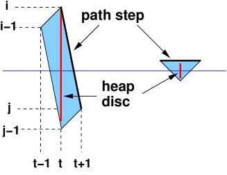
Figure 16. The path-heap correspondence. To each descending step $(t,i)\to(t+1,j)$ of any path on $\Gamma_{\mathbf{M}}$, we associate the parallelogram indicated. The corresponding heap disc is a segment on the vertical diagonal of the parallelogram. To each double horizontal step we associate the triangle indicated. The corresponding heap disc is on the vertical median of the triangle.

Given a graph $\Gamma_{\mathbf{M}}$, we represent paths on the graph from $0$ to $0$ on the two-dimensional lattice as before. We advance by one step in the “time” ($x$) direction for each step in the path, and record the height of the vertex visited in the vertical coordinate.

Associate to each descending step $(t,i)\to(t+1,j)$ in this picture the parallellogram with vertices $\{(t,i),(t+1,j)(t,j-1)(t-1,i-1)\}$, and represent a vertical segment $\{(t,x),\ x\in[j-1+\epsilon,i-\epsilon]\}$ for $\epsilon>0$ sufficiently small (see Fig.16). For double horizontal steps (steps of the form $(t-1,i)\to(t,i)\to(t+1,i)$), we draw the half-diamond with vertices $\{(t-1,i),(t+1,i),(t,i-1)\}$, and the segment $\{(t,x),\ x\in[i-1+\epsilon,i-\epsilon]\}$ for $\epsilon>0$ sufficiently small. These segments represent the discs of the heap.

The heap graph $G_{\mathbf{M}}$ encodes the overlap between these segments. the vertices of $G_{\mathbf{M}}$ are in bijection with the descending steps on $\Gamma_{\mathbf{M}}$, and the edges connect any pair of steps such that the associated discs cannot freely slide horizontally without touching each-other. Weights on the vertices are assigned according to edge weights.

To construct $G_{\mathbf{M}}$ directly from ${\mathbf{M}}$, we proceed as for $\Gamma_{\mathbf{M}}$. We associate a graph $G_{{\mathbf{m}}_{i}}$ to each strictly decending piece ${\mathbf{m}}_{i}$ of ${\mathbf{M}}$. We then glue these pieces according to the type of separating step between them.

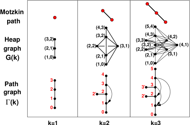
Figure 17. The heap graphs $G(k)$ corresponding to the strictly descending Motzkin paths with $k=1,2,3$ vertices, together with the corresponding path target graphs $\Gamma(k)$. The vertices of $G(k)$ are indexed by the descending steps on $\Gamma(k)$.

Let ${\mathbf{m}}$ be a strictly descending Motzkin path with $k$ vertices. Let $G_{\mathbf{m}}=G(k)$. Its vertices are indexed by the descending steps on $\Gamma(k)$. The descending steps on $\Gamma(k)$ are indexed by $(i,j)$ for $i=j=2,3,...,k$, $i=j+1=1,2,...,k+2$ and $k+1\geq i>j+1\geq 2$, hence $G(k)$ has a total of $k-1+k+2+k(k-1)/2=(k+1)(k+2)/2$ vertices. The descending steps $k+2\to k+1$ and $1\to 0$ are singled out, and form the top and bottom vertices of $G(k)$, denoted by $t$ and $b$.

The descending step $(i,j)$ ($i\geq j$) overlaps with any descending step $(m,\ell)$ ($m\geq\ell$) such that $m$ or $\ell\in[j,i]$ (or both). The set of all these overlapping descending steps $(i,j)-(m,\ell)$ forms the edges of $G(k)$. We have represented the graphs $G(k)$ for $k=1,2,3$ in Fig.17, together with the path graphs $\Gamma(k)$ of Fig.12 for $k=1,2,3$.

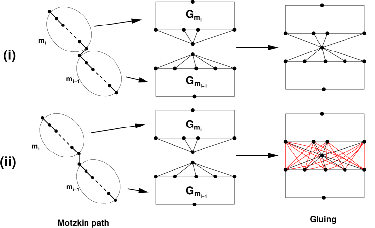
Figure 18. The heap graphs $G_{{\mathbf{m}}_{i-1}}$ and $G_{{\mathbf{m}}_{i}}$ corresponding to the strictly descending Motzkin paths ${\mathbf{m}}_{i-1}$ and ${\mathbf{m}}_{i}$ are glued in two possible ways, according to whether the Motzkin paths are separated by (i) a step $(1,1)$ or (ii) a step $(0,1)$. Both involve identifying the top vertex of $G_{{\mathbf{m}}_{i-1}}$ with the bottom vertex of $G_{{\mathbf{m}}_{i}}$, but in the case (ii) all the vertices connected to the bottom vertex of $G_{{\mathbf{m}}_{i}}$ must be connected to all the vertices connected to the top vertex of $G_{{\mathbf{m}}_{i-1}}$.

The graphs $G_{{\mathbf{m}}_{i-1}}$ and $G_{{\mathbf{m}}_{i}}$ are glued in two possible ways, according to whether ${\mathbf{m}}_{i-1}$ and ${\mathbf{m}}_{i}$ are separated by a step $(1,1)$ (type (i)) or $(0,1)$ (type (ii)) (see Fig.18):

• Type (i): The top vertex $t_{i-1}$ of $G_{{\mathbf{m}}_{i-1}}$ is identified with the bottom vertex $b_{i}$ of $G_{{\mathbf{m}}_{i}}$.

• Type (ii): The top vertex $t_{i-1}$ of $G_{{\mathbf{m}}_{i-1}}$ is identified with the bottom vertex $b_{i}$ of $G_{{\mathbf{m}}_{i}}$, and all the vertices connected to $t_{i-1}$ are connected to all the vertices connected to $b_{i}$, via additional edges.

Example 5.9.

Consider $\mu_{1}(G_{3})$ of Figure 36 of Appendix A (top of second column from left). The corresponding Motzkin path is $\{(1,1),(0,2),(0,3)\}$, and has two strictly descending pieces ${\mathbf{m}}_{1}=\{(1,1),(0,2)\}$ and ${\mathbf{m}}_{2}=\{(0,3)\}$. The graphs $G_{{\mathbf{m}}_{1}}$ and $G_{{\mathbf{m}}_{2}}$ correspond to the vertices denoted $\{1,2,3,4,5,8\}$ and $\{5,6,7\}$ respectively in Fig.36. As they are glued according to the rule (ii), all the vertices connected to $5$ in $G_{{\mathbf{m}}_{1}}$, namely $4$ and $8$, are connected to all the vertices connected to $5$ in $G_{{\mathbf{m}}_{2}}$, namely $6$.

Remark 5.10.

Let us define the overlap between descending edges of $\Gamma_{{\mathbf{M}}}$ as follows: the descending edge $(i,j)$ ($i\geq j$) overlaps the descending edge $(m,\ell)$ ($m\geq\ell$) if and only if $m$ or $\ell\in[j,i]$ (or both). We may now bypass the above gluing procedure by directly associating to $\Gamma_{\mathbf{M}}$ the graph $G_{\mathbf{M}}$ as follows: (i) the vertices of $G_{{\mathbf{M}}}$ are in bijection with the descending edges on $\Gamma_{\mathbf{M}}$ and (ii) the edges of $G_{\mathbf{M}}$ connect all pairs of vertices such that the corresponding descending edges overlap.

The bijection between paths on $\Gamma_{\mathbf{M}}$ and heaps on $G_{\mathbf{M}}$ follows as before from decomposing any heap into shells of successive foregrounds, and the fact that there is a unique way of arranging the discs (and their surrounding parallelograms) on the square lattice from bottom to top and left to right in each shell, and filling the spaces in-between with ascending steps of the path.

6. Path interpretation of $R_{1,n}$ and cluster mutations

Path partition functions give a combinatorial interpretation for $\{R_{1,n}\}$, expressed in terms of any cluster seed in the fundamental domain. For each Motzkin path ${\mathbf{M}}$, $F_{1}^{(r)}(t)=\sum_{n\geq 0}t^{n}R_{1,n}$ is a path partition function on a graph $\Gamma_{\mathbf{M}}$ with positive weights depending on ${\mathbf{x}}_{\mathbf{M}}$. This results in a positivity theorem for all $\{R_{1,n}\}_{n\in{\mathbb{Z}}}$, as well as explicit expressions for the generating function.

6.1. Path partition functions in terms of transfer matrices

6.1.1. Path transfer matrix

Let $\mathcal{P}_{\mathbf{M}}^{(n)}(a,b)$ be the set of paths on the graph $\Gamma_{\mathbf{M}}$ starting at vertex $a$ and ending at vertex $b$ with $n$ descending steps. The partition function is

(6.1) $$Z_{\mathbf{M}}^{(n)}(a,b)=\sum_{p\in\mathcal{P}_{\mathbf{M}}^{(n)}(a,b)}\prod_{e\in p}y_{e}({\mathbf{M}}).$$

(Recall that only descending edges have non-trivial weights). Define the generating function

(6.2) $$Z_{\mathbf{M}}(a,b)=\sum_{n\geq 0}t^{n}\,Z_{\mathbf{M}}^{(n)}(a,b).$$

This can be computed by use of the transfer matrix $T_{\mathbf{M}}$, the weighted incidence matrix of $\Gamma_{\mathbf{M}}$, with an additional factor $t$ per descending step. Its rows and columns are indexed by the vertices of $\Gamma_{\mathbf{M}}$ (the ordering on vertices is such that $i<i^{\prime}<i+1$), with non-vanishing entries

$$(T_{\mathbf{M}})_{i,j}=\left\{\begin{matrix}1&\hbox{if $j\to i$ is an ascending edge},\\ ty_{j,i}&\hbox{if $j\to i$ is a descending edge}.\end{matrix}\right.$$

where $y_{j,i}$ is the weight of the oriented edge $j\to i$. We have

(6.3) $$Z_{\mathbf{M}}(a,b)=\left((I-T_{\mathbf{M}})^{-1}\right)_{b,a}$$

where $I$ is the identity matrix.

Let $F_{\mathbf{M}}(t):=Z_{\mathbf{M}}(0,0)$. The entry $((I-T_{\mathbf{M}})^{-1})_{0,0}$ is computed by row-reduction, using upper unitriangular row operations to obtain a lower triangular matrix, then taking the $(0,0)$ entry of the latter. To be precise, we iterate the following procedure:

1. Let $t$ be the last row in the matrix $A$. Define the matrix $A^{\prime}$ with entries

   $$A^{\prime}_{i,j}=A_{i,j}-{A_{i,{\rm t}}A_{{\rm t},j}\over A_{{\rm t},{\rm t}}},\quad i<t.$$

   Then $A^{\prime}_{i,{\rm t}}=0$ for all $i<{\rm t}$.

2. Truncate $A^{\prime}$ by deleting its last row and column.

Repeat this until the result is a $1\times 1$ matrix, which is $1/(A^{-1})_{0,0}$.

For our particular set of graphs, the reduction procedure has a graphical interpretation. It gives the partition function in terms of a pruned graph with the top part removed, and replaced by a single “loop” with a different weight, corresponding to the partition function on the pruned branch.

Example 6.1.

The transfer matrix of the graph ${\tilde{K}}_{2}$ of Figure 12 is

(6.4) $$T_{{\tilde{K}}_{2}}={\small\left(\begin{matrix}0&ty_{1}&0&0&0&0\\ 1&0&ty_{2}&0&ty_{3,1}&0\\ 0&1&0&ty_{3}&ty_{4}&0\\ 0&0&1&0&0&0\\ 0&0&1&0&0&ty_{5}\\ 0&0&0&0&1&0\\ \end{matrix}\right)}$$

with vertex order $(0,1,2,2^{\prime},3,4)$. Note that $y_{3,1}=y_{2}y_{4}/y_{3}$ due to (5.2). The reduction of $A=I-T_{{\tilde{K}}_{2}}$ is

$$I-T_{{\tilde{K}}_{2}} \to {\small\left(\begin{matrix}1&-ty_{1}&0&0&0\\ -1&1&-ty_{2}&0&-ty_{3,1}\\ 0&-1&1&-ty_{3}&-ty_{4}\\ 0&0&-1&1&0\\ 0&0&-1&0&1-ty_{5}\\ \end{matrix}\right)}\to{\small\left(\begin{matrix}1&-ty_{1}&0&0\\ -1&1&-ty_{2}-{ty_{3,1}\over 1-ty_{5}}&0\\ 0&-1&1-{ty_{4}\over 1-ty_{5}}&-ty_{3}\\ 0&0&-1&1\\ \end{matrix}\right)}$$

$$\to {\small\left(\begin{matrix}1&-ty_{1}&0\\ -1&1&-ty_{2}-{ty_{3,1}\over 1-ty_{5}}\\ 0&-1&1-ty_{3}-{ty_{4}\over 1-ty_{5}}\\ \end{matrix}\right)}\to{\small\left(\begin{matrix}1&-ty_{1}\\ -1&1-t{y_{2}+{y_{3,1}\over 1-ty_{5}}\over 1-ty_{3}-{ty_{4}\over 1-ty_{5}}}\\ \end{matrix}\right)}$$

$$\to 1-{ty_{1}\over 1-t{y_{2}+{y_{3,1}\over 1-ty_{5}}\over 1-ty_{3}-{ty_{4}\over 1-ty_{5}}}}={1\over\left((I-T_{{\tilde{K}}_{2}})^{-1})\right)_{0,0}}$$

This is identical to the inverse of the factor of $tR_{1,1}$ in the second term of eq.(4.14), upon identifying $z_{i}=y_{i}$, $i=1,2,3,4,5$ and $z_{6}=y_{3,1}$.

6.1.2. Block structure

To see how this works in general, we now describe the structure of $T_{\mathbf{M}}$. It consists of blocks which are put together according to the gluing procedure.

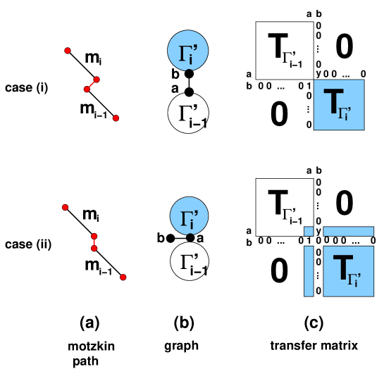
Figure 19. Construction of the transfer matrix $T_{\mathbf{M}}$ in the case of (i) vertical and (ii) horizontal gluing of the subgraphs $\Gamma_{m_{i-1}}^{\prime}$ and $\Gamma_{m_{i}}^{\prime}$. (a) Is the motzkin path, (b) is the graph gluing and (c) the gluing of the two diagonal blocks $T_{\Gamma_{i-1}^{\prime}}$ and $T_{\Gamma_{i}^{\prime}}$. We have shaded the graph $\Gamma_{i}^{\prime}$ in (b) and the corresponding matrix elements of the block $T_{\Gamma_{i}^{\prime}}$ in (c). The added element $y$ stands for the weight $ty_{b,a}$ in both cases (i) and (ii).

Recall the decomposition of ${\mathbf{M}}$ into strictly descending pieces ${\mathbf{m}}_{i}$. Let $\Gamma^{\prime}_{{\mathbf{m}}_{i}}$ be the graph with its bottom and top vertices and edges removed. Define $T^{\prime}_{{\mathbf{m}}_{i}}$ to be the transfer matrix of $\Gamma_{{\mathbf{m}}_{i}}^{\prime}$. Let also $\Gamma_{{\mathbf{m}}_{0}}^{\prime}$ and $\Gamma_{{\mathbf{m}}_{p+1}}^{\prime}$ denote the bottom and top vertices, glued via vertical edges to $\Gamma^{\prime}_{{\mathbf{m}}_{1}}$ and $\Gamma^{\prime}_{{\mathbf{m}}_{p}}$. We write $\Gamma_{\mathbf{M}}=\Gamma^{\prime}_{{\mathbf{m}}_{0}}||\Gamma^{\prime}_{{\mathbf{m}}_{1}}||\cdots||\Gamma^{\prime}_{{\mathbf{m}}_{p+1}}$ to denote the gluing procedure. (Gluing via the operation $||$ consists of adding a vertical edge or a horizontal edge and vertex.)

The matrix $T_{\mathbf{M}}$ is obtained by gluing the diagonal blocks $T_{\Gamma_{i}^{\prime}}$ according to whether the corresponding graph gluing is via a (i) vertical or (ii) horizontal edge (see Figure 19):

$\bullet$ Type (i): The blocks $T_{\Gamma_{i-1}^{\prime}}$ and $T_{\Gamma_{i}^{\prime}}$ occupy successive diagonal blocks in the matrix $T_{\mathbf{M}}$ (vertex $t_{i-1}^{\prime}$ of $\Gamma_{i-1}^{\prime}$ is followed by vertex $b^{\prime}_{i}$ of $T_{\Gamma_{i}^{\prime}}$). They are “glued” by the addition of two matrix elements, $(T_{\mathbf{M}})_{b^{\prime}_{i},t^{\prime}_{i-1}}=1$ and $(T_{\mathbf{M}})_{t^{\prime}_{i-1},b^{\prime}_{i}}=y=ty_{b^{\prime}_{i},t^{\prime}_{i-1}}$.

$\bullet$ Type (ii): We place the two blocks $T_{\Gamma_{i-1}^{\prime}}$ and $T_{\Gamma_{i}^{\prime}}$ in the matrix $T_{\mathbf{M}}$ in such a way that the last row and column of $T_{\Gamma_{i-1}^{\prime}}$ (with index $t^{\prime}_{i-1}$) coincide with the first row and column of $T_{\Gamma_{i}^{\prime}}$ (with index $b_{i}^{\prime}$). We then insert a new row and column labeled $b_{i}$ following $t^{\prime}_{i-1}$, with nonvanishing entries $(T_{\mathbf{M}})_{b_{i},t^{\prime}_{i-1}}=1$ and $(T_{\mathbf{M}})_{t^{\prime}_{i-1},b_{i}}=y=ty_{b_{i},t^{\prime}_{i-1}}$.

6.2. Reduction and continued fractions

6.2.1. General reduction process

Now consider the reduction procedure performed on the matrix $A=I-T_{\mathbf{M}}$.

1. Let $(t^{\prime},{\rm t})$ denote the last two row indices of $A$. The bottom right $2\times 2$ submatrix of $I-T_{\mathbf{M}}$ has the form $\left(\begin{matrix}1&-y\\ -1&1\end{matrix}\right)$ with $y=ty_{{\rm t},t^{\prime}}=ty_{2r+1}$. Reduction erases the row and column ${\rm t}$ of $A$, and replaces $A_{t^{\prime},t^{\prime}}=1\mapsto 1-y$.

2. Inductive step: After reduction of all rows with index $j>t^{\prime}_{i}$, the resulting matrix $T_{\Gamma_{{\mathbf{m}}_{0}}^{\prime}||\cdots||\Gamma_{i}^{\prime}}^{\prime}$ differs from the original only in the element $(t^{\prime}_{i},t^{\prime}_{i})$, denoted by $\gamma_{i}$, where

   $$(1-\gamma_{i})^{-1}=\left((I-T_{\Gamma_{\{{t^{\prime}}_{i}\}}||\Gamma_{i+1}^{\prime}||\cdots||\Gamma_{p+1}^{\prime}})^{-1}\right)_{{t^{\prime}}_{i},{t^{\prime}}_{i}}\ .$$

   We then reduce all indices $j>t^{\prime}_{i-1}+1$. This results in the matrix $A^{\prime}$. Its lower right $2\times 2$ matrix, indexed by the vertices $a,b$, has the form:

   Case (i): $\left(\begin{matrix}1&-y\\ -1&1-c\end{matrix}\right)$ where $y=ty_{b,a}$ and $(1-c)^{-1}=\left((I-T_{\Gamma_{i}^{\prime}||\cdots||\Gamma_{p+1}^{\prime}})^{-1}\right)_{b,b}$. One more reduction step eliminates row and column $b$ and gives the new entry $A_{a,a}\mapsto 1-{y\over 1-c}$.

   Case (ii): $\left(\begin{matrix}1-c&-y\\ -1&1\end{matrix}\right)$. One more step in the reduction gives $A_{a,a}\mapsto 1-y-c$.

   In both cases, the net result is a modification of $A$ in which the bottom right element is $1-\gamma_{i-1}$, where

   $$(1-\gamma_{i-1})^{-1}=\left((I-T_{\Gamma_{\{{t^{\prime}}_{i-1}\}}||\Gamma_{i}^{\prime}||\cdots||\Gamma_{p+1}^{\prime}})^{-1}\right)_{{t^{\prime}}_{i-1},{t^{\prime}}_{i-1}}\ .$$

   The bottom right element of the reduced transfer matrix is $\gamma_{i-1}$ equal to (i) $y/(1-c)$ or (ii) $y+c$.

6.2.2. The case of a strictly descending Motzkin path

Consider the transfer matrix corresponding to $\Gamma(k)^{\prime}$ (Figure 12)). For later use, we use a more general matrix $T^{\prime}(k)$, which has $T(k)^{\prime}_{k+1,k+1}=c$ instead of 0. With vertex order $(1,2,2^{\prime},3,3^{\prime},...,k,k^{\prime},k+1)$, this matrix is

(6.5) $$T^{\prime}(k)={\small\left(\begin{array}[]{lllllllllll}0&ty_{2}&0&ty_{3,1}&0&ty_{4,1}&0&\cdots&ty_{k,1}&0&ty_{k+1,1}\\ 1&0&ty_{3}&ty_{4}&0&ty_{4,2}&0&\cdots&ty_{k,2}&0&ty_{k+1,2}\\ 0&1&0&0&0&0&0&\cdots&0&0&0\\ 0&1&0&0&ty_{5}&ty_{6}&0&\cdots&ty_{k,3}&0&ty_{k+1,3}\\ 0&0&0&1&0&0&0&\cdots&0&0&0\\ 0&0&0&1&0&0&ty_{7}&\cdots&ty_{k,4}&0&ty_{k+1,4}\\ \vdots&\vdots&\vdots&\vdots&\vdots&\vdots&\vdots&\ddots&\vdots&\vdots&\vdots\\ 0&0&0&0&0&0&0&\cdots&0&ty_{2k-1}&ty_{2k}\\ 0&0&0&0&0&0&0&\cdots&1&0&0\\ 0&0&0&0&0&0&0&\cdots&1&0&c\\ \end{array}\right)}$$

Reduction of the last index in $A=(I-T^{\prime}(k))$ results in

$$\left\{\begin{array}[]{ll}y_{k,i}\mapsto y_{k,i}+{y_{k+1,i}\over 1-c}&\hbox{in row $i<k-1$};\\ y_{2k-2}\mapsto y_{2k-2}+{y_{k+1,k-1}\over 1-c}&\hbox{in row $k-1$};\\ A_{kk}\mapsto 1-t{y_{2k}\over 1-c}&\hbox{in row $k$}.\end{array}\right.$$

whereas reduction of the next index changes $A_{kk}^{\prime}=1-ty_{2k}/(1-c)\mapsto 1-ty_{2k-1}-t{y_{2k}\over 1-c}$.

Let

(6.6) $$\varphi_{k}(y_{2},...,y_{2k};y_{3,1},y_{4,1},...,y_{k+1,k-1};c)=\Big{(}(I-T^{\prime}(k))^{-1}\Big{)}_{1,1}$$

As a result of the two reduction steps, $\varphi_{k}$ is replaced by $\varphi_{k-1}$, with suitable substitutions of variables.

Lemma 6.2.

The function $\varphi_{k}=\left((I-T^{\prime}_{\Gamma(k)^{\prime}})^{-1}\right)_{1,1}$ is determined by the recursion relation

$$\varphi_{k}(\{y_{j}\}_{j=2}^{2k};\{y_{j,i}\}_{2\leq i+1<j\leq k+1};c)$$

$$\ \ \ \ \ \ \ \ =\varphi_{k-1}(\{y_{j}+\delta_{j,2k-2}{y_{k+1,k-1}\over 1-c}\}_{j=2}^{2k-2};\{y_{j,i}+\delta_{j,k}{y_{k+1,i}\over 1-c}\}_{2\leq i+1<j\leq k};ty_{2k-1}+t{y_{2k}\over 1-c}),$$

with

(6.7) $$\varphi_{1}(y_{2};\ ;c)=\left(\left(\begin{matrix}1&-ty_{2}\\ -1&1-c\end{matrix}\right)^{-1}\right)_{1,1}={1\over 1-t{y_{2}\over 1-c}}.$$

Example 6.3.

For $k=2$, we have

$$\varphi_{2}(y_{2},y_{3},y_{4};y_{3,1};c)=\varphi_{1}\left(y_{2}+{y_{3,1}\over 1-c};\ ;ty_{3}+{ty_{4}\over 1-c}\right)={1\over 1-{ty_{2}+{ty_{3,1}\over 1-c}\over 1-ty_{3}-{ty_{4}\over 1-c}}}$$

For $k=3$, we have:

$$\varphi_{3}(y_{2},y_{3},y_{4},y_{5},y_{6};y_{3,1},y_{4,1},y_{4,2};c) = \varphi_{2}\left(y_{2},y_{3},y_{4}+{y_{4,2}\over 1-c};y_{3,1}+{y_{4,1}\over 1-c};ty_{5}+{ty_{6}\over 1-c}\right)$$

$$= {1\over 1-{ty_{2}+{ty_{3,1}+{ty_{4,1}\over 1-c}\over 1-ty_{5}-{ty_{6}\over 1-c}}\over 1-ty_{3}-{ty_{4}+{ty_{4,2}\over 1-c}\over 1-ty_{5}-t{y_{6}\over 1-c}}}}$$

Thus, $\varphi_{k}$ is a finite, multiply branched continued fraction. Its power series expansion in $t$ has coefficients which are polynomials in the weights with non-negative integer coefficients. This expression is still valid if we relax the proportionality conditions (5.2), but if we use these for $j=1$, we see that

(6.8) $$\varphi_{k}={1\over 1-{y_{2}\over y_{3}}{ty_{3}+ty_{4}w_{k}\over 1-ty_{3}-ty_{4}w_{k}}}$$

where $w_{k}$ does not depend on $y_{2},y_{3},y_{4}$.

6.3. Mutations as fraction rearrangements

6.3.1. Mutations and Motzkin paths

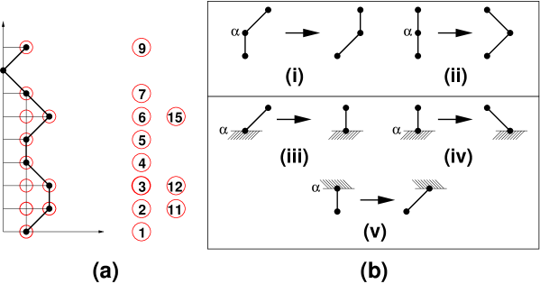
Figure 20. A path ${\mathbf{M}}$ with $r=9$ (a), and the product of mutations (circled) yielding ${\mathbf{M}}$ when applied on ${\mathbf{M}}_{0}$. In (b), the two generic moves (i) and (ii) corresponding to the actions of the mutation are indicated, together with their “boundary” version, (iii) and (iv) when ${\alpha}=1$, and (v) when ${\alpha}=r$.

One can associate a unique sequence of mutations to each Motzkin path ${\mathbf{M}}$ using the following procedure. The path ${\mathbf{M}}=\{(m_{\alpha},{\alpha})\}_{{\alpha}\in I_{r}}$ is considered on the lattice, and each lattice point $(x,{\alpha})$ with $1\leq x\leq m_{\alpha}$ corresponds to a mutation $\mu_{\alpha}\ (\mu_{{\alpha}+r})$ if $x$ is odd (even), respectively. The compound mutation $\mu$ such that $\mu({\mathbf{x}}_{0})={\mathbf{x}}_{M}$ is the product of these mutations read from bottom to top, and from right to left. For example, in Figure 20 (a), $\mu=\mu_{11}\mu_{12}\mu_{15}\mu_{1}\mu_{2}\mu_{3}\mu_{4}\mu_{5}\mu_{6}\mu_{7}\mu_{9}$.

This restricted set of mutations acting on ${\mathbf{M}}_{0}$ yields any path ${\mathbf{M}}$ in the fundamental domain. We need to use only the two elementary moves shown in Figure 20 (b) (i)–(ii), and their “boundary” versions (iii)–(v). Without loss of generality we may therefore restrict ourselves to this subset of mutations.

To see how this set of mutations acts on the partition function, we compare the graphs and weights $(\Gamma_{\mathbf{M}},{\mathbf{y}}({\mathbf{M}}))$ and $(\Gamma_{{\mathbf{M}}^{\prime}},{\mathbf{y}}({\mathbf{M}}^{\prime}))$, where ${\mathbf{M}}^{\prime}=\mu_{\alpha}({\mathbf{M}})$ or $\mu_{{\alpha}+r}({\mathbf{M}})$.

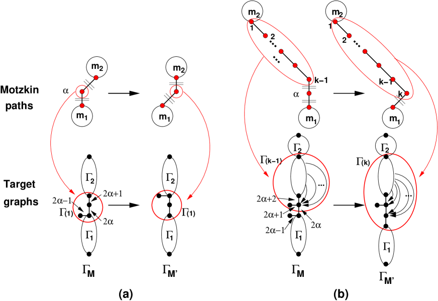
Figure 21. The two bulk moves of Fig.20 (b) acting on the paths and graphs. The edges involved in the transformation are indicated. The mutation (a) involves the three edges of the center piece $\Gamma(1)$, and is independent of the structure of ${\mathbf{m}}_{1}$ and ${\mathbf{m}}_{2}$. Mutation (b) involves four edges, and depends on the length of the strictly descending subpath above vertex ${\alpha}+1$, increasing its length by 1. On the graph it transforms the block $\Gamma(k-1)$ into $\Gamma(k)$, creating $k$ new descending edges.

6.3.2. Bulk mutations of type (a) and (b)

Consider first the two bulk moves (i)-(ii) of Figure 20 (b). Their effect on the corresponding target graphs is shown in Figure 21 (a) and (b). The path ${\mathbf{M}}$ is decomposed into a vertex labeled ${\alpha}$, and bottom and top pieces ${\mathbf{m}}_{1}$ and ${\mathbf{m}}_{2}$, corresponding to graphs $\Gamma(1)$, $\Gamma_{1}$ and $\Gamma_{2}$ respectively.

In Figure 21 (a), the edge labels of the piece $\Gamma(1)$ corresponding to the central isolated vertex ${\alpha}$ of ${\mathbf{M}}$ are identified, they are $2{\alpha}-1,2{\alpha}$ and $2{\alpha}+1$ We find that all the independent edge weights in $\Gamma_{\mathbf{M}}$ and $\Gamma_{{\mathbf{M}}^{\prime}}$ are identical, except for the three weights $y_{2{\alpha}-1},y_{2{\alpha}},y_{2{\alpha}+1}$ of $\Gamma_{\mathbf{M}}$. These transform to $y_{2{\alpha}-1}^{\prime},y_{2{\alpha}}^{\prime},y_{2{\alpha}+1}^{\prime}$ in $\Gamma_{{\mathbf{M}}^{\prime}}$. As we shall see below, the new weights correspond to the mutation of cluster variables.

The matrix $A_{\mathbf{M}}=1-T_{\Gamma_{\mathbf{M}}}$, after the reduction of the block corresponding to $\Gamma_{2}$, becomes:

(6.9) $${\small\left(\begin{array}[]{c|cc|c}\hbox{\Large$I-T_{\Gamma_{1}}$}&\begin{matrix}0\\ \vdots\\ 0\\ -ty_{2{\alpha}-1}\end{matrix}&\begin{matrix}0\\ \vdots\\ 0\\ -ty_{2{\alpha}}\end{matrix}&\hbox{\Large$0$}\\ \hline\cr 0\ \cdots\ 0\ -1&1&0&0\ \hskip 14.45377pt\cdots\hskip 14.45377pt\ 0\\ 0\ \cdots\ 0\ -1&0&1&-ty_{2{\alpha}+1}\ 0\ \cdots\ 0\\ \hline\cr\hbox{\Large$0$}&\begin{matrix}0\\ 0\\ \vdots\\ 0\end{matrix}&\begin{matrix}1\\ 0\\ \vdots\\ 0\end{matrix}&\hbox{\Large$I-T_{\Gamma_{2}}$}\\ \end{array}\right)}\mapsto{\small\left(\begin{array}[]{c|cc|c}\hbox{\Large$I-T_{\Gamma_{1}}$}&\begin{matrix}0\\ \vdots\\ 0\\ -ty_{2{\alpha}-1}\end{matrix}&\begin{matrix}0\\ \vdots\\ 0\\ -ty_{2{\alpha}}\end{matrix}&\begin{matrix}0\\ \vdots\\ 0\\ 0\end{matrix}\\ \hline\cr 0\ \cdots\ 0\ -1&1&0&0\\ 0\ \cdots\ 0\ -1&0&1&-ty_{2{\alpha}+1}\\ \hline\cr 0\ \cdots\ 0\ \ \ \ \ 0&0&-1&1-c^{\prime}\\ \end{array}\right)}$$

with $(1-c^{\prime})^{-1}=\Big{(}(I-T_{\Gamma_{2}})^{-1}\Big{)}_{b_{2},b_{2}}$ ($b_{2}$ is the bottom vertex of $\Gamma_{2}$). Three more iterations of reduction replace the bottom right element of $I-T_{\Gamma_{1}}$ with

(6.10) $$f=1-{ty_{2{\alpha}-1}-{ty_{2{\alpha}}\over 1-{ty_{2{\alpha}+1}\over 1-c^{\prime}}}}\ .$$

Similarly, reduction of $I-T_{\Gamma_{{\mathbf{M}}^{\prime}}}$ yields (after reducing the $\Gamma_{2}$ part)

(6.11) $$I-T_{\Gamma_{{\mathbf{M}}^{\prime}}}\mapsto{\small\left(\begin{array}[]{c|ccc}\hbox{\huge$I-T_{\Gamma_{1}}$}&\begin{matrix}0\\ \vdots\\ 0\\ -ty_{2{\alpha}-1}^{\prime}\end{matrix}&\begin{matrix}0\\ \vdots\\ 0\\ 0\end{matrix}&\begin{matrix}0\\ \vdots\\ 0\\ 0\end{matrix}\\ \hline\cr 0\ 0\ \cdots\ 0\ -1&1&-ty_{2{\alpha}}^{\prime}&0\\ 0\ 0\ \cdots\ 0\ \ \ \ \ 0&-1&1-c^{\prime}&-ty_{2{\alpha}+1}^{\prime}\\ 0\ 0\ \cdots\ 0\ \ \ \ \ 0&0&-1&1\\ \end{array}\right)}$$

with $c^{\prime}$ as above. Three more reduction iterations result in the updated bottom right element of $I-T_{\Gamma_{1}}$,

(6.12) $$f^{\prime}=1-{ty_{2{\alpha}-1}^{\prime}\over 1-{ty_{2{\alpha}}^{\prime}\over 1-ty_{2{\alpha}+1}^{\prime}-c^{\prime}}}\ .$$

The partition functions of paths on $\Gamma_{\mathbf{M}}$ and $\Gamma_{{\mathbf{M}}^{\prime}}$ must coincide, they are the same partition function expressed in terms of different variables. They coincide if and only if the weights $y^{\prime}_{2{\alpha}-1},y^{\prime}_{2{\alpha}},y^{\prime}_{2{\alpha}+1}$ are such that $f=f^{\prime}$ (all the other weights are equal). Application of the rearrangement Lemma 4.6, with $a=y_{2{\alpha}-1}$, $b=y_{2{\alpha}}$, $c=y_{2{\alpha}+1}$ and $d=c^{\prime}$, gives $f=f^{\prime}$ if and only if:

(6.13) $$y_{2{\alpha}-1}^{\prime}=y_{2{\alpha}-1}+y_{2{\alpha}},\quad y_{2{\alpha}}^{\prime}={y_{2{\alpha}}y_{2{\alpha}+1}\over y_{2{\alpha}-1}+y_{2{\alpha}}},\quad y_{2{\alpha}+1}^{\prime}={y_{2{\alpha}-1}y_{2{\alpha}+1}\over y_{2{\alpha}-1}+y_{2{\alpha}}}\ .$$

We interpret this transformation as the effect of the mutation $\mu_{\alpha}$ or $\mu_{{\alpha}+r}$ on the skeleton weights of $\Gamma_{\mathbf{M}}$, resulting in a rearrangement of the continued fraction $F_{\mathbf{M}}(t)$ into $F_{{\mathbf{M}}^{\prime}}(t)$.

The mutation in Figure 21 (b) is slightly more subtle, because it depends on the length of the strictly descending subpath in ${\mathbf{m}}$ above ${\alpha}$, whose length is increased by 1. All independent edge weights are unaffected by the mutation, except those of edges $2{\alpha}-1,...,2{\alpha}+2$ (recall that the other edge weights are ratios of skeleton weights $y_{1},y_{2},...,y_{2r+1}$).

The transfer matrix is

(6.14) $$T_{\mathbf{M}}={\small\left(\begin{array}[]{c|c|l}\hbox{\Large$T_{\Gamma_{1}}$}&\begin{matrix}0\\ \vdots\\ 0\\ ty_{2{\alpha}-1}\end{matrix}&\begin{matrix}\begin{matrix}0\\ \vdots\\ 0\\ ty_{2{\alpha}}\end{matrix}&\ \ \ \ \hbox{\huge$0$}\end{matrix}\\ \hline\cr 0\ 0\ \cdots\ 0\ 1&0&0\hskip 36.135pt\cdots\hskip 36.135pt0\\ \hline\cr\begin{matrix}\\ \hbox{\huge$0$}\end{matrix}&\begin{matrix}\\ 0\\ \vdots\\ 0\end{matrix}&\hbox{\Large$T_{\Gamma_{\hbox{\small$y_{2{\alpha}+1},y_{2{\alpha}+2}$}}(k-1)|\Gamma_{2}}$}\\ \end{array}\right)},$$

where $\Gamma_{y_{2{\alpha}+1},y_{2{\alpha}+2}}(k-1)$ is the circled graph in $\Gamma_{\mathbf{M}}$, on the bottom of Fig.21 (b), for which we indicate the values of the weights of its first two lowest edges. After reduction, we are left with $(I-T_{\Gamma_{1}})$, with the bottom diagonal element replaced by

(6.15) $$f=1-ty_{2{\alpha}-1}-{ty_{2{\alpha}}\over 1-c(y_{2{\alpha}+1},y_{2{\alpha}+2})}\ ,$$

where $(1-c(y_{2{\alpha}+1},y_{2{\alpha}+2}))^{-1}=\Big{(}(I-T_{\Gamma_{y_{2{\alpha}+1},y_{2{\alpha}+2}}(k-1)|\Gamma_{2}})^{-1}\Big{)}_{b^{\prime},b^{\prime}}$, where $b^{\prime}$ denotes the next-to-bottom vertex of $\Gamma(k-1)$.

On the other hand,

(6.16) $$T_{{\mathbf{M}}^{\prime}}={\small\left(\begin{array}[]{c|c|l}\hbox{\huge$T_{\Gamma_{1}}$}&\begin{matrix}0\\ \vdots\\ 0\\ ty_{2{\alpha}-1}^{\prime}\end{matrix}&\begin{matrix}\begin{matrix}0\\ \vdots\\ 0\\ 0\end{matrix}&\ \ \ \ \hbox{\huge$0$}\end{matrix}\\ \hline\cr 0\ 0\ \cdots\ 0\ 1&0&ty_{2{\alpha}}^{\prime}\ 0\ *\ 0\ *\ 0\ \cdots\ 0\ *\\ \hline\cr\hbox{\huge$0$}&\begin{matrix}1\\ 0\\ \vdots\\ 0\end{matrix}&\hbox{\huge$T_{\Gamma_{\hbox{\small$y_{2{\alpha}+1}^{\prime},y_{2{\alpha}+2}^{\prime}$}}(k-1)|\Gamma_{2}}$}\\ \end{array}\right)}$$

where the entries $*$ stand for matrix elements of the form $ty_{j,i}^{\prime}$, where the vector $(ty_{2{\alpha}}^{\prime},(ty_{j,i}^{\prime}))$ is proportional to the vector $(ty_{2{\alpha}+1}^{\prime},ty_{2{\alpha}+2}^{\prime},(ty_{j,i}))$, which are the weights appearing in the row below it. This fact can be used to eliminate the $*$ entries using the row below. Then the reduction gives the matrix

(6.17) $${\small\left(\begin{array}[]{c|cc}\hbox{\huge$I-T_{\Gamma_{1}}$}&\begin{matrix}0\\ \vdots\\ 0\\ ty_{2{\alpha}-1}^{\prime}\end{matrix}&\begin{matrix}0\\ \vdots\\ 0\\ 0\end{matrix}\\ \hline\cr 0\ 0\ \cdots\ 0\ -1&1+{y_{2{\alpha}}^{\prime}\over y_{2{\alpha}+1}^{\prime}}&-{y_{2{\alpha}}^{\prime}\over y_{2{\alpha}+1}^{\prime}}\\ 0\ 0\ \cdots\ 0\ \ \ \ 0&-1&1-c(y_{2{\alpha}+1}^{\prime},y_{2{\alpha}+2}^{\prime})\end{array}\right)}$$

where $\Big{(}1-c(y_{2{\alpha}+1}^{\prime},y_{2{\alpha}+2}^{\prime})\Big{)}^{-1}=\Big{(}(I-T_{\Gamma_{y_{2{\alpha}+1}^{\prime},y_{2{\alpha}+2}^{\prime}}(k-1)|\Gamma_{2}})^{-1}\Big{)}_{b^{\prime},b^{\prime}}$, with $c$ as in (6.15). Two further reduction steps replace the bottom right element of $(I-T_{\Gamma_{1}})$ by

(6.18) $$f^{\prime}=1-{ty_{2{\alpha}-1}^{\prime}\over 1-{y_{2{\alpha}}^{\prime}\over y_{2{\alpha}+1}^{\prime}}{c(y_{2{\alpha}+1}^{\prime},y_{2{\alpha}+2}^{\prime})\over 1-c(y_{2{\alpha}+1}^{\prime},y_{2{\alpha}+2}^{\prime})}}\ .$$

The partition functions for graphs on $\Gamma_{\mathbf{M}}$ and $\Gamma_{{\mathbf{M}}^{\prime}}$ must be equal, so we look for the transformation $(y_{2{\alpha}-1},y_{2{\alpha}},y_{2{\alpha}+1},y_{2{\alpha}+2})\to(y_{2{\alpha}-1}^{\prime},y_{2{\alpha}}^{\prime},y_{2{\alpha}+1}^{\prime},y_{2{\alpha}+2}^{\prime})$ such that $f=f^{\prime}$.

The function $c^{\prime}=c(y_{2{\alpha}+1}^{\prime},y_{2{\alpha}+2}^{\prime})$ is identified by row-reducing $(I-T_{\Gamma(k)|\Gamma_{2}})$. Reducing the $\Gamma_{2}$ part results in replacing the bottom right element of $(I-T_{\Gamma(k)})$ with $1-d^{\prime}$, where $(1-d^{\prime})^{-1}=\Big{(}(I-T_{\Gamma_{2}})^{-1}\Big{)}_{b_{2},b_{2}}$. This yields the relation $1-{y_{2{\alpha}}^{\prime}\over y_{2{\alpha}+1}^{\prime}}{c^{\prime}\over 1-c^{\prime}}=\varphi_{k}^{-1}(y_{2{\alpha}}^{\prime},y_{2{\alpha}+1}^{\prime},y_{2{\alpha}+2}^{\prime},y_{2{\alpha}+3}...,y_{2{\alpha}+2k-2};\{y_{j,i}\};d^{\prime})$, with $\varphi_{k}$ as in Lemma 6.2, and we get $c^{\prime}=y_{2{\alpha}+1}^{\prime}+w_{k}y_{2{\alpha}+2}^{\prime}$, by comparison with the general expression (6.8). Therefore

(6.19) $$f=1-ty_{2{\alpha}-1}-{ty_{2{\alpha}}\over 1-ty_{2{\alpha}+1}-ty_{2{\alpha}+2}w_{k}}=f^{\prime}=1-{ty_{2{\alpha}-1}^{\prime}\over 1-{y_{2{\alpha}}^{\prime}\over y_{2{\alpha}+1}^{\prime}}{ty_{2{\alpha}+1}^{\prime}+ty_{2{\alpha}+2}^{\prime}w_{k}\over 1-ty_{2{\alpha}+1}^{\prime}+ty_{2{\alpha}+2}^{\prime}w_{k}}}\ .$$

Applying the rearrangement Lemma 4.6 with $a=y_{2{\alpha}-1}$, $b=y_{2{\alpha}}$ and $c=y_{2{\alpha}+1}+y_{2{\alpha}+2}w_{k}$, we conclude that (6.19) is satisfied if and only if

(6.20) $$y_{2{\alpha}-1}^{\prime}=y_{2{\alpha}-1}+y_{2{\alpha}},\quad y_{2{\alpha}}^{\prime}={y_{2{\alpha}}y_{2{\alpha}+1}\over y_{2{\alpha}-1}+y_{2{\alpha}}},\quad y_{2{\alpha}+1}^{\prime}={y_{2{\alpha}-1}y_{2{\alpha}+1}\over y_{2{\alpha}-1}+y_{2{\alpha}}},\quad y_{2{\alpha}+2}^{\prime}={y_{2{\alpha}+2}y_{2{\alpha}-1}\over y_{2{\alpha}-1}+y_{2{\alpha}}}\ ,$$

while all other weights $y^{\prime}_{i}$ are equal to $y_{i}$. This is interpreted as the effect of the mutation $\mu_{\alpha}$ or $\mu_{r+{\alpha}}$ on the graph weights.

6.3.3. Boundary mutations

We consider the mutations of Fig.20 (b) (iii-v).

$\bullet$ Case (v). We have ${\alpha}=r$, which is just case (a) of Fig.21, with ${\mathbf{m}}_{2}=\emptyset$ and $\Gamma_{2}$ reduced to a vertex. The transformation of weights is (6.13).

$\bullet$ Cases (iii-iv). Here, ${\alpha}=1$. We take ${\mathbf{m}}_{1}=\emptyset$ and $\Gamma_{1}$ a single vertex in both cases (a) and (b) of Figure 21. However, the action of $\mu_{1}$ or $\mu_{r+1}$ introduces a new feature, which we call re-rooting. This is because the effect of the mutation is an application of the rearrangement Lemma 4.6 on the corresponding weighted path partition function $F_{\mathbf{M}}(t)$. This is possible only if the graph $\Gamma_{\mathbf{M}}$ is rooted at vertex $b^{\prime}=1$ instead of vertex $b=0$. We write $F_{{\mathbf{M}}}(t)=1+ty_{1}({\mathbf{M}})F^{\prime}_{{\mathbf{M}}}(t)$, where $F_{\mathbf{M}}(t)=\Big{(}(I-T_{{\mathbf{M}}})^{-1}\Big{)}_{0,0}$, while $F^{\prime}_{{\mathbf{M}}}(t)=\Big{(}(I-T_{{\mathbf{M}}})^{-1}\Big{)}_{1,1}$.

This re-rooting must take place whenever we act via the moves (iii-iv) as a direct consequence of the cases (a) and (b) of Fig.21. Indeed, $\Gamma_{1}$ is reduced to a vertex. The lower edge $2{\alpha}-1=1$ is horizontal, and the vertex common with $\Gamma_{1}$ is $b^{\prime}=1$, rather than $b=0$, so that $\Gamma_{1}=\{b^{\prime}\}$. The weight $y_{1}$ of the horizontal edge is associated with the step $0\to 1$ in the re-rooted formulation.

In general, the weighted path partition function $F_{\mathbf{M}}(t)$, corresponding to the Motzkin path ${\mathbf{M}}$, is related to the initial generating function $F_{{\mathbf{M}}_{0}}(t)=R_{1,0}^{-1}F_{1}^{(r)}(t)$, via the following sequence of re-rootings. We start from the canonical sequence of Motzkin paths leading from ${\mathbf{M}}_{0}$ to ${\mathbf{M}}=(m_{1},...)$ via our restricted set of mutations. Within this sequence, the paths ${\mathbf{M}}^{(i_{\ell})}$, $\ell=1,2,...,m_{1}$ are those which differ from their predecessor only in via the action of the “boundary” mutations $\mu_{1}$ or $\mu_{r+1}$. Note that $m_{1}({\mathbf{M}}_{\ell})=\ell$. Only the boundary mutations $\mu_{1}$ and $\mu_{r+1}$ imply a re-rooting (otherwise $F_{{\mathbf{M}}^{(i-1)}}=F_{{\mathbf{M}}^{(i)}}$). Thus,

Lemma 6.4.

The partition function $F_{\mathbf{M}}(t)$ is obtained from $F_{{\mathbf{M}}_{0}}(t)=R_{1,0}^{-1}F_{1}^{(r)}(t)$ via the sequence of re-rootings:

$$F_{{\mathbf{M}}_{\ell-1}}(t)=1+ty_{1}({\mathbf{M}}_{\ell-1})F_{{\mathbf{M}}_{\ell}}(t),\ \ \ell=1,2,...,m_{1}$$

with $F_{\mathbf{M}}=F_{{\mathbf{M}}_{m_{1}}}$, where $m_{1}=m_{1}({\mathbf{M}})$ is the first entry of ${\mathbf{M}}=(m_{\alpha},{\alpha})_{{\alpha}=1}^{r}$.

This allows to interpret $R_{1,n+m_{1}}({\mathbf{x}}_{\mathbf{M}})$, expressed as a function of the cluster variable ${\mathbf{x}}_{\mathbf{M}}$, in terms of the partition function $F_{\mathbf{M}}(t)$. Let us denote by $F(t)\Big{|}_{t^{n}}$ the coefficient of $t^{n}$ in the series $F(t)$.

Lemma 6.5.

$$R_{1,n+m_{1}}=R_{1,0}F_{{\mathbf{M}}_{0}}(t)\Big{|}_{t^{n+m_{1}}}=R_{1,0}\,y_{1}({\mathbf{M}}_{0})y_{1}({\mathbf{M}}_{1})...y_{1}({\mathbf{M}}_{m_{1}})\,F_{\mathbf{M}}(t)\Big{|}_{t^{n}}$$

Proof.

We use Lemma 6.4. The prefactor is obtained by collecting the successive multiplicative weights of each re-rooting. ∎

6.3.4. Main theorem

Let us summarize the results of this section in the following:

Theorem 6.6.

The mutation of cluster variables $\mu_{\alpha}$ or $\mu_{{\alpha}+r}:{\mathbf{x}}_{\mathbf{M}}\to{\mathbf{x}}_{{\mathbf{M}}^{\prime}}$ is equivalent to a rearrangement relating the continued fractions $F_{\mathbf{M}}\to F_{{\mathbf{M}}^{\prime}}$ that generate weighted paths on the rooted target graphs $\Gamma_{\mathbf{M}}$ and $\Gamma_{{\mathbf{M}}^{\prime}}$. The edge weights of the corresponding skeleton trees, ${\mathbf{y}}({\mathbf{M}})=\{y_{1}({\mathbf{M}}),...,y_{2r+1}({\mathbf{M}})\}$ and ${\mathbf{y}}^{\prime}={\mathbf{y}}({\mathbf{M}}^{\prime})$ are related through either of the two transformations (6.13) or (6.20), while all other weights remain the same.

6.4. Weights and the mutation matrix $B$

There is a simple expression for the edge weights of $\Gamma_{\mathbf{M}}$ in terms of the cluster variables ${\mathbf{x}}_{\mathbf{M}}$ and the mutation matrix $B({\mathbf{M}})$ at the seed ${\mathbf{M}}$. To specify all the edge weights $\Gamma_{\mathbf{M}}$, one need only specify $y_{1}({\mathbf{M}}),y_{2}({\mathbf{M}}),...,y_{2r+1}({\mathbf{M}})$, due to the relations (5.2) for the other weights.

Theorem 6.7.

The weights $y_{1}({\mathbf{M}}),y_{2}({\mathbf{M}}),...,y_{2r+1}({\mathbf{M}})$ of the skeleton tree $\Gamma_{\mathbf{M}}$ are the following Laurent monomials of the cluster variable ${\mathbf{x}}_{\mathbf{M}}$:

(6.21) $$y_{2{\alpha}-1}({\mathbf{M}}) = {\lambda_{{\alpha},m_{\alpha}}\over\lambda_{{\alpha}-1,m_{{\alpha}-1}}}\ ,\ ({\alpha}=1,2,...,r+1),$$

$$y_{2{\alpha}}({\mathbf{M}}) = {\mu_{{\alpha}+1,m_{\alpha}+1}\over\mu_{{\alpha},m_{{\alpha}}}}\left(1-\delta_{m_{\alpha},m_{{\alpha}+1}+1}(1-{\lambda_{{\alpha}+1,m_{{\alpha}+1}}\over\lambda_{{\alpha}+1,m_{{\alpha}}}})\right)$$

$$\hskip 72.26999pt\times\left(1-\delta_{m_{{\alpha}-1},m_{{\alpha}}+1}(1-{\lambda_{{\alpha}-1,m_{{\alpha}}}\over\lambda_{{\alpha}-1,m_{{\alpha}-1}}})\right)\ ,\ ({\alpha}=1,2,...,r),$$

where

(6.23) $$\lambda_{{\alpha},n}={R_{{\alpha},n+1}\over R_{{\alpha},n}},\qquad\mu_{{\alpha},n}={R_{{\alpha},n}\over R_{{\alpha}-1,n}}.$$

Proof.

Weights are determined by their initial values (3.17) at seed ${\mathbf{M}}_{0}$ and by the recursion relations (6.13) (in the case $m_{{\alpha}-1}=m_{\alpha}<m_{{\alpha}+1}$) and (6.20) (in the case $m_{{\alpha}-1}=m_{\alpha}=m_{{\alpha}+1}$) for each mutation in our restricted set, all other weights being invariant.

Using the $Q$-system (1.4), one checks that the relations (6.13) and (6.20) are satisfied by the weights (6.21) and (6.7). ∎

Note that eqs.(6.21)-(6.7) involve only the data $(R_{{\alpha},m_{\alpha}},R_{{\alpha},m_{{\alpha}+1}})_{{\alpha}=1}^{r}$, the cluster variables at the seed ${\mathbf{M}}$.

Example 6.8.

Consider ascending Motzkin paths as in Example 5.6. The weights from Theorem 6.7 are

(6.24) $$y_{2{\alpha}-1}({\mathbf{M}}) = {\lambda_{{\alpha},m_{\alpha}}\over\lambda_{{\alpha}-1,m_{{\alpha}-1}}}\ ,\quad y_{2{\alpha}}({\mathbf{M}})={\mu_{{\alpha}+1,m_{\alpha}+1}\over\mu_{{\alpha},m_{{\alpha}}}}\ ,$$

since only mutations of type (a) of the previous subsection are used. In the particular case of ${\mathbf{M}}={\mathbf{M}}_{0}$, Equations (6.24) reduce to (3.17).

In the case of the strictly ascending path ${\mathbf{M}}_{max}=(0,1,...,r-1)$, with cluster variables $(R_{{\alpha},{\alpha}-1},R_{{\alpha},{\alpha}})_{{\alpha}\in I_{r}}$,

(6.25) $$x_{2{\alpha}-1}:=y_{2{\alpha}-1}({\mathbf{M}}_{max})={R_{{\alpha}-1,{\alpha}-2}R_{{\alpha},{\alpha}}\over R_{{\alpha}-1,{\alpha}-1}R_{{\alpha},{\alpha}-1}},\quad x_{2{\alpha}}:=y_{2{\alpha}}({\mathbf{M}}_{max})={R_{{\alpha}-1,{\alpha}-1}R_{{\alpha}+1,{\alpha}}\over R_{{\alpha},{\alpha}-1}R_{{\alpha},{\alpha}}}\ .$$

The graph $\Gamma_{{\mathbf{M}}_{max}}={\tilde{H}}_{r}$, the chain of $2r+2$ vertices. The partition function is

(6.26) $$F_{{\mathbf{M}}_{max}}(t)=F_{1}^{(r)}(t)=\sum_{n\geq 0}t^{n}R_{1,n}={R_{1,0}\over 1-t{x_{1}\over 1-t{x_{2}\over 1-t{x_{3}\over\ \ \ \ \ {\ddots\over 1-t{x_{2r}\over 1-tx_{2r+1}}}}}}}$$

Remark 6.9.

Recalling the discrete Wronskian expression $R_{{\alpha},n}=\det_{1\leq i,j\leq{\alpha}}(R_{1,n+i+j-{\alpha}-1})$, we may view the result (6.25)-(6.26) as a particular case of a theorem of Stieltjes [23] (see also [1]), which expresses the formal power series expansion $F(\lambda)=\sum_{k\geq 0}(-1)^{k}a_{k}/\lambda^{k+1}$ around $\infty$ for any sequence $a_{k}$, $k\in{\mathbb{Z}}_{\geq 0}$, as the continued fraction

$$F(\lambda)={1\over\beta_{1}\lambda+{1\over\beta_{2}+{1\over\beta_{3}\lambda+\cdots}}}$$

where $\beta_{2k}=(\Delta_{k}^{0})^{2}/(\Delta_{k}^{1}\Delta_{k-1}^{1})$, $\beta_{2k+1}=(\Delta_{k}^{1})^{2}/(\Delta_{k}^{0}\Delta_{k+1}^{0})$, and

(6.27) $$\Delta_{k}^{m}=\det_{1\leq i,j\leq k}(a_{m+i+j-2})$$

are Hankel determinants involving the sequence $a_{k}$. Indeed, writing $\lambda=-1/t$ and taking $a_{k}=R_{1,k}$, we easily identify the two continued fraction expressions $F(\lambda)$ and $F_{1}^{(r)}(t)$ of eq.(6.26) upon taking $x_{k}={1\over\beta_{k}\beta_{k+1}}$, while $1/\beta_{1}=a_{0}=R_{1,0}$ yields the overall prefactor. Note that the continued fraction is actually finite, as $1/\beta_{2r+3}\propto\Delta_{r+2}^{0}=0$.

The weights computed in Theorem 6.7 are simply related to the exchange matrix $B({\mathbf{M}})$ of the cluster algebra at the seed ${\mathbf{M}}$.

Theorem 6.10.

The exchange matrix $B({\mathbf{M}})$ at the point ${\mathbf{M}}=\{(m_{\alpha},{\alpha})\}_{{\alpha}=1}^{r}$ reads, for $1\leq i,j\leq r$:

(6.28) $$B({\mathbf{M}})_{i,j} =(-1)^{\lfloor{m_{j}+1\over 2}\rfloor}\left((-1)^{\lfloor{m_{i}\over 2}\rfloor}-(-1)^{\lfloor{m_{j}\over 2}\rfloor}\right)\delta_{|i-j|,1}$$

$$B({\mathbf{M}})_{i,j+r} =(-1)^{\lfloor{m_{i}+1\over 2}\rfloor+\lfloor{m_{j}\over 2}\rfloor+1}C_{i,j}$$

$$B({\mathbf{M}})_{i+r,j} =(-1)^{\lfloor{m_{i}\over 2}\rfloor+\lfloor{m_{j}+1\over 2}\rfloor}C_{i,j}$$

$$B({\mathbf{M}})_{i+r,j+r} =(-1)^{\lfloor{m_{i}\over 2}\rfloor}\left((-1)^{\lfloor{m_{j}+1\over 2}\rfloor}-(-1)^{\lfloor{m_{i}+1\over 2}\rfloor}\right)\delta_{|i-j|,1}$$

where $C$ is the Cartan matrix of $A_{r}$.

Proof.

By induction. The theorem is true when ${\mathbf{M}}={\mathbf{M}}_{0}$, where $B_{{\mathbf{M}}_{0}}=\left(\begin{matrix}0&-C^{t}\\ C&0\end{matrix}\right)$.

Assuming it is true for some ${\mathbf{M}}$ with $m_{{\alpha}-1}=m_{\alpha}\leq m_{{\alpha}+1}$, let us prove it for ${\mathbf{M}}^{\prime}$, with $m^{\prime}_{\beta}=m_{\beta}+\delta_{\beta,{\alpha}}$. We distinguish according to the parity of $m_{\alpha}$: if $m_{\alpha}$ is even, we use the mutation $\mu_{\alpha}$, otherwise we use $\mu_{{\alpha}+r}$.

Assume $m_{\alpha}$ even. Under the mutation $\mu_{\alpha}$, the matrix elements $B({\mathbf{M}})_{i,{\alpha}}$ and $B({\mathbf{M}})_{{\alpha},j}$ are negated. This is compatible with Equation (6.28) by noting that $\lfloor{m_{\alpha}^{\prime}\over 2}\rfloor=\lfloor{m_{\alpha}\over 2}\rfloor$ and that $\lfloor{m_{\alpha}^{\prime}+1\over 2}\rfloor=\lfloor{m_{\alpha}+1\over 2}\rfloor+1$, which gives the expected extra minus sign. For the other entries of $B(M)$, we use (1.8):

$$B({\mathbf{M}}^{\prime})_{i,j}=B({\mathbf{M}})_{i,j}+{\rm sgn}(B({\mathbf{M}})_{i,{\alpha}})[B({\mathbf{M}})_{i,{\alpha}}B({\mathbf{M}})_{{\alpha},j}]_{+}$$

with $i,j\neq{\alpha}$. Assume $j\leq r$. Then $B({\mathbf{M}})_{{\alpha},j}\neq 0$ only if $\lfloor{m_{j}\over 2}\rfloor={m_{\alpha}\over 2}\pm 1$, while $|i-{\alpha}|=|j-{\alpha}|=1$. Due to the Motzkin path condition, this is only possible if $m_{j}=m_{\alpha}-1$, but is impossible, as we must have $m_{{\alpha}+1},m_{{\alpha}-1}\geq m_{\alpha}$. Therefore $B_{i,j}({\mathbf{M}})=B_{i,j}({\mathbf{M}}^{\prime})$. Similarly, if $i\leq r$, we have the same conclusion.

If $i,j>r$, we write $i=i^{\prime}+r$ and $j=j^{\prime}+r$, with $i^{\prime},j^{\prime}\leq r$. Then

$$B({\mathbf{M}})_{i^{\prime}+r,{\alpha}}B({\mathbf{M}})_{{\alpha},j^{\prime}+r}=-C_{i^{\prime},{\alpha}}C_{{\alpha},j^{\prime}}(-1)^{\lfloor{m_{i^{\prime}}\over 2}\rfloor+\lfloor{m_{j^{\prime}}\over 2}\rfloor}$$

is positive only if $i^{\prime}={\alpha}$ and $j^{\prime}={\alpha}\pm 1$, in which case (i) $m_{j^{\prime}}=m_{\alpha}$ or (ii) $j^{\prime}={\alpha}+1$ and $m_{j^{\prime}}=m_{{\alpha}+1}=m_{\alpha}+1$, (or with $i^{\prime}$ and $j^{\prime}$ interchanged). Then $B({\mathbf{M}})_{i^{\prime}+r,{\alpha}}B({\mathbf{M}})_{{\alpha},j^{\prime}+r}=2$. In the case (i), we have $B_{{\alpha}+r,j^{\prime}+r}({\mathbf{M}})=0$, hence $B_{{\alpha}+r,j^{\prime}+r}({\mathbf{M}}^{\prime})=0+2=2$, compatible with Equation (6.28), as $\lfloor{m_{\alpha}^{\prime}+1\over 2}\rfloor=\lfloor{m_{\alpha}+1\over 2}\rfloor+1$. In the case (ii), we have $B_{{\alpha}+r,{\alpha}+1+r}({\mathbf{M}})=-2$, hence $B_{{\alpha}+r,{\alpha}+1+r}({\mathbf{M}}^{\prime})=-2+2=0$, also in agreement with Equation (6.28), as ${m_{{\alpha}+1}+1\over 2}={m_{\alpha}\over 2}+1=\lfloor{m_{\alpha}^{\prime}+1\over 2}\rfloor$.

The case of $m_{\alpha}$ odd is treated analogously. ∎

Remark 6.11.

It is interesting to note that the $B$-matrices of Theorem 6.10 only have entries in $\{0,\pm 1,\pm 2\}$. This is true only for the cluster subgraph ${\mathcal{G}}_{r}$, as the entries grow arbitrarily in the complete cluster graph ${\mathbb{T}}_{2r}$. We also note the remarkable property, that the sum of the four blocks $r\times r$ of the $B$-matrices always vanishes, namely that $B_{i,j}+B_{i+r,j}+B_{i,j+r}+B_{i+r,j+r}=0$ for $i,j=1,2,...,r$.

The sequence $\Big{(}(R_{{\alpha},m_{\alpha}})_{{\alpha}=1}^{r},(R_{{\alpha},m_{\alpha}+1})_{{\alpha}=1}^{r}\Big{)}$ and the sequence of cluster variables $x_{\mathbf{M}}=(R_{\rm even},R_{\rm odd})\equiv(x_{i}({\mathbf{M}}))_{i=1}^{2r}$ (where the $R_{{\alpha},m}$ are listed first for the even entries in $m$ and then for the odd ones) are related via a permutation $\sigma_{\mathbf{M}}$:

(6.29) $$\sigma_{\mathbf{M}}({\alpha})=\left\{\begin{matrix}{\alpha}&{\rm if}\ m_{\alpha}\ {\rm is}\ {\rm even}\\ {\alpha}+r&{\rm if}\ m_{\alpha}\ {\rm is}\ {\rm odd},\ {\rm and}\ {\alpha}\leq r\\ {\alpha}-r&{\rm if}\ m_{\alpha}\ {\rm is}\ {\rm odd},\ {\rm and}\ {\alpha}>r\end{matrix}\right.$$

We have the following expression:

Theorem 6.12.

The weights computed in Theorem 6.7 are related to the exchange matrix of the cluster algebra $B({\mathbf{M}})$:

(6.30) $${y_{2{\alpha}-1}({\mathbf{M}})\over y_{2{\alpha}}({\mathbf{M}})}=\prod_{i=1}^{2r}x_{i}({\mathbf{M}})^{B({\mathbf{M}})_{i,\sigma_{\mathbf{M}}({\alpha})}},\qquad{y_{2{\alpha}}({\mathbf{M}})\over y_{2{\alpha}+1}({\mathbf{M}})}=\prod_{i=1}^{2r}x_{i}({\mathbf{M}})^{B({\mathbf{M}})_{i,\sigma_{\mathbf{M}}({\alpha}+r)}},~{}({\alpha}\in I_{r}.)$$

6.5. Positivity of the cluster variables $R_{1,n}$

The variables $R_{1,n}$ can now be shown to be positive Laurent polynomials of any possible set of cluster variables ${\mathbf{x}}_{\mathbf{M}}$. Note that the graphs $\Gamma_{\mathbf{M}}$ are invariant under translations of ${\mathbf{M}}$, but the same is not true the weights ${\mathbf{y}}({\mathbf{M}})$.

Theorem 6.13.

For any Motzkin path ${\mathbf{M}}=\{(m_{\alpha},{\alpha})\}_{{\alpha}=1}^{r}$ with $r$ vertices and any $n\geq 0$, the solution $R_{1,n+m_{1}}({\mathbf{x}}_{\mathbf{M}})$ of the $A_{r}$ $Q$-system, expressed as a function of ${\mathbf{x}}_{\mathbf{M}}$, is equal to $R_{1,m_{1}}$ times the generating function for weighted paths on $\Gamma_{\mathbf{M}}$, starting and ending at the root, with $n$ down steps, and with weights $y_{e}({\mathbf{M}})$ given by Theorem 6.7, namely:

$$R_{1,n+m_{1}}({\mathbf{x}}_{\mathbf{M}})=R_{1,m_{1}}\,F_{\mathbf{M}}(t)\Big{|}_{t^{n}}$$

Moreover, $R_{1,n+m_{1}}$ is expressed as an explicit Laurent polynomial of the cluster variable ${\mathbf{x}}_{\mathbf{M}}$, with non-negative integer coefficients, for all $n\in{\mathbb{Z}}$.

Proof.

By Theorem 2.4, we can restrict ourselves to the Motzkin paths of the fundamental domain. The first statement of the Theorem follows from Lemma 6.5, with the prefactor $R_{1,0}y_{1}({\mathbf{M}}_{0})...y_{1}({\mathbf{M}}_{p})=R_{1,m_{1}}$, by use of (6.21) for ${\alpha}=1$.

The second statement is clear for $n\geq 0$. It is a direct consequence of the reinterpretation of $R_{1,n+m_{1}}$ as the generating function for weighted paths with n down steps, for all $n\geq 0$, by also noting that the weights $y_{e}({\mathbf{M}})$ are all positive Laurent monomials of the initial data, as a consequence of Theorem 6.7.

For $n<0$, we simply use an enhanced version of the reflection property of Lemma 2.1. Indeed, noting that the $Q$-system equations are invariant under the reflection $n\to-n$, we deduce that the quantity $R_{1,n+m_{1}}$, expressed as a function of the initial data ${\mathbf{x}}_{{\mathbf{M}}}$, is the same as $R_{1,-n-m_{1}}$ expressed as a function of the reflected initial data ${\mathbf{x}}_{{\mathbf{M}}^{t}}$, where the reflected Motzkin path ${\mathbf{M}}^{t}=\{(m_{\alpha}^{t},{\alpha})\}$ satisfies $m_{\alpha}^{t}=-(m_{\alpha}+1)$ for ${\alpha}=1,2,...,r$. In other words, if $R_{1,n+m_{1}}=f({\mathbf{x}}_{\mathbf{M}})$, then $R_{1,-n-m_{1}}=f({\mathbf{x}}_{{\mathbf{M}}^{t}})$.

Let us now use the translation invariance of the $Q$-system in the form of eq.(2.5). We first translate the reflected Motzkin path ${\mathbf{M}}^{t}$ back to the fundamental domain, namely so that its lowest entry $m_{\alpha}^{t}$ be zero. This is done by considering $m^{t}={\rm Min}_{{\alpha}=1,2,...,r}(m_{\alpha}^{t})$, and the translate ${\mathbf{M}}^{\prime}={\mathbf{M}}^{t}-m^{t}$, with entries $m_{\alpha}^{\prime}=m_{\alpha}^{t}-m^{t}$ for all ${\alpha}$. Then for $n<0$, the quantity $R_{1,-n-m_{1}+m^{t}}$ is still given by the same expression as before in terms of the shifted Motzkin path ${\mathbf{M}}^{\prime}$, namely $R_{1,-n-m_{1}+m^{t}}=f({\mathbf{x}}_{{\mathbf{M}}^{\prime}})$. But now the first part of the Theorem applies, as $m_{1}^{\prime}=m_{1}({\mathbf{M}}^{\prime})=-m_{1}-1-m^{t}$. Indeed, as $-n+1\geq 0$, we deduce that $R_{1,-n+1+m_{1}^{\prime}}=f({\mathbf{x}}_{{\mathbf{M}}^{\prime}})$ is a positive Laurent polynomial of the reflected-translated data ${\mathbf{x}}_{{\mathbf{M}}^{\prime}}$. As $R_{1,n+m_{1}}=f({\mathbf{x}}_{{\mathbf{M}}})$ via the same function $f$, we conclude that $R_{1,n+m_{1}}$ is also a positive Laurent polynomial of the initial data ${\mathbf{x}}_{\mathbf{M}}$, for all $n<0$. This completes the proof of the Theorem. ∎

In view of the correspondence between path partition functions on $\Gamma_{\mathbf{M}}$ and heap partition functions on $G_{\mathbf{M}}$, we have also

Corollary 6.14.

The weighted heap graph $G_{\mathbf{M}}$ associated to the Motzkin path ${\mathbf{M}}$ is constructed as above. The heaps on $G_{\mathbf{M}}$ with $n$ discs are in bijection with the weighted paths on $\Gamma_{\mathbf{M}}$ with $n$ descending steps, starting and ending at the root. For any Motzkin path ${\mathbf{M}}$ and any $n\geq 0$, the quantity $R_{1,n+m_{1}}$ is expressed in terms of the cluster variable ${\mathbf{x}}_{\mathbf{M}}$ as $R_{1,m_{1}}$ times the partition function for weighted heaps with $n$ discs on $G_{\mathbf{M}}$.

7. Strongly non-intersecting path interpretation of $R_{{\alpha},n}$

We now provide a combinatorial interpretation of the determinant expressions for $R_{{\alpha},n}$ (${\alpha}>1$) as partition functions of families of strongly non-intersecting paths on $\Gamma_{\mathbf{M}}$. For this, we need to generalize the usual notion of non-intersecting lattice paths. As a result we obtain a proof of the positivity of the determinant expression for $R_{{\alpha},n}$ with ${\alpha}>1$.

7.1. Ascending Motzkin paths: Paths on trees $T_{2r+2}(I)$

First consider the case of the ascending Motzkin paths. The graphs $\Gamma_{\mathbf{M}}$ are skeleton trees, as in Section 5.6, denoted by $T_{2r+2}(I)$ where $I=\{i_{1},i_{2},\ldots,i_{s}\}$ with $1<i_{1}<i_{2}<\cdots<i_{s}<2r-s$ and $i_{1}-1$, $i_{2}-i_{1}$,…$i_{s}-i_{s-1}$ odd. The variables $R_{1,n}$ are partition functions of paths on these trees, starting and ending at vertex 0.

Paths on $T_{2r+2}(I)$ are equivalent to paths on the two-dimensional lattice, with the $y$-coordinate restricted to $0\leq y\leq 2r+1-s$, with the following possible steps: (i) $(x,y)\to(x+1,y+1)$; (ii) $(x,y)\to(x+1,y-1)$ and (iii) $(x,y)\to(x+2,y)$ ($y\in I$).

We say that two such paths intersect if they share a vertex.

Theorem 7.1.

Let $n\geq{\alpha}-1$. Then $R_{{\alpha},n}$ is $(R_{1,0})^{\alpha}$ times the partition function of families of ${\alpha}$ non-intersecting paths on $T_{2r+2}(I)$, starting at the points $(0,0),(2,0),...,(2{\alpha}-2,0)$ and ending at the points $(2n,0),(2n+2,0),...,(2n+2{\alpha}-2,0)$, with weights as in Example 6.8.

Proof.

We apply the Lindström-Gessel-Viennot (LGV) theorem [19, 11]. Consider the partition function $Z_{A_{1},...,A_{\alpha}}^{E_{1},...,E_{\alpha}}$ of non-intersecting families of ${\alpha}$ weighted paths from the initial points $A_{1},A_{2},...,A_{\alpha}$ to endpoints $E_{1},E_{2},...,E_{\alpha}$. We assume that if $i<j$ and $k<l$, then a path $A_{i}\to E_{l}$ must intersect any path $A_{j}\to E_{k}$. Let $Z_{A_{i}\to E_{j}}$ be the partition function for weighted paths from $A_{i}$ to $E_{j}$, then

(7.1) $$Z_{A_{1},...,A_{\alpha}}^{E_{1},...,E_{\alpha}}=\det_{1\leq i,j\leq{\alpha}}\left(Z_{A_{i}\to E_{j}}\right)$$

Now, $R_{1,n}$ is $R_{1,0}$ times the partition function of paths on $T_{2r+2}(I)$ from $(0,0)$ to $(2n,0)$. Let $A_{i}=(2i-2,0)$ and $E_{i}=(2n+2{\alpha}-2i,0)$ ($i=1,2,...,{\alpha}$). Since ${Z}_{A_{i}\to E_{j}}$ is the partition function for paths of $2n+2{\alpha}-2i-2j+2$ time-steps, it may be identified with $R_{1,n+{\alpha}-i-j+1}/R_{1,0}$. We conclude that

(7.2) $$Z_{A_{1},...,A_{\alpha}}^{E_{1},...,E_{\alpha}}={1\over(R_{1,0})^{\alpha}}\det_{1\leq i,j\leq{\alpha}}\left(R_{1,n+{\alpha}-i-j+1}\right)={R_{{\alpha},n}\over(R_{1,0})^{\alpha}}$$

where we have used Lemma (2.6). ∎

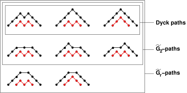
Figure 22. The eight pairs of non-intersecting ${\tilde{G}}_{r}$-paths of $8$ and $4$ time-steps for $r\geq 3$. The top box contains the non-intersecting ${\tilde{H}}_{r}$- (Dyck-) paths. There are six pairs of paths on $\widetilde{G}_{2}$.

Example 7.2.

For ${\alpha}=2$, $n=2$ and $r\geq 3$,

$$R_{2,3}=R_{1,4}R_{1,2}-(R_{1,3})^{2}= = x_{1}^{2}x_{2}x_{3}(x_{1}x_{3}+x_{1}x_{4}+x_{2}x_{4})$$

$$= y_{1}^{2}y_{2}(y_{1}y_{3}^{2}+2y_{1}y_{3}y_{4}+y_{1}y_{4}^{2}+(y_{1}+y_{2})y_{4}(y_{5}+y_{6}))$$

with $x_{i}$ as in (6.25) and $y_{i}$ as in (3.17). The first expression corresponds to the three pairs of paths in the top of Figure 22. The second expression corresponds to the eight pairs of non-intersecting ${\tilde{G}}_{r}$-paths of $8$ and $4$ time-steps depicted in Figure 22. We also indicated in this figure the six pairs of non-intersecting paths on ${\tilde{G}}_{2}$, for which no horizontal step at height $3$ is allowed, eliminating the two configurations of the bottom row.

7.2. Strongly non-intersecting paths on $\Gamma_{\mathbf{M}}$

Theorem 7.1 can be generalized to paths on $\Gamma_{\mathbf{M}}$ even when $\Gamma_{\mathbf{M}}$ is not a tree. To do this, we must generalize the notion of non-intersecting paths, using a representation of $\Gamma_{\mathbf{M}}$-paths on the two-dimensional lattice which preserves the property that the number of descending steps is half the horizontal length of the path. (Note that this representation is different from the one used in Figure 16.)

7.2.1. Two-dimensional representation of $\Gamma_{\mathbf{M}}$-paths

Figure 23. The two-dimensional path representation of a path on $\Gamma_{\mathbf{M}}$ with ${\mathbf{M}}=(2,1,0)$ (see Figure 12 with $r=3$). Descents of height $2$ are vertical (horizontal displacement $2-h=0$), while descents of height $3$ go back one step horizontally ($2-h=-1$). With this choice, the horizontal distance between the starting and ending point is twice the number of descents ($16=2\times 8$ here).

Some of the descending steps on $\Gamma_{\mathbf{M}}$ may have height $h>1$, in case there is an edge $j\to i$ with $j-i>1$. When $h=0$ or $1$, each descending step is in bijection with an ascending one, but this is not true if $h>1$. We require that the total horizontal displacement in a path $i\to i+1\to\cdots\to j-1\to j\to i$ should be independent of the height $h=j-i$ of descending step used. Therefore, on the two-dimensional lattice, we draw a descent along an edge of length $h$ as a line from $(x,y)$ to $(x-h+2,y-h)$. Then a path which goes up $h$ single steps, then down one step of height $h$ has horizontal length $2$, independently of $h$.

With this convention, the horizontal distance between the start and end of a path from the 0 to 0 on $\Gamma_{\mathbf{M}}$ is twice the number of its descending steps (see Figure 23 for an illustration).

Definition 7.3.

The two-dimensional representation of a path with $n$ descents on $\Gamma_{\mathbf{M}}$ is a path in $({\mathbb{Z}}_{+})^{2}$, starting at $(0,0)$ and ending at $(2n,0)$, with the possible steps:

• $(x,y)\to(x+1,y+1)$ whenever there is an edge $y\to y+1$ in $\Gamma_{\mathbf{M}}$.

• $(x,y)\to(x+2,y)$ whenever there is an edge $y\to y^{\prime}\to y$ in $\Gamma_{\mathbf{M}}$.

• $(x,y)\to(x+2-h,y-h)$, $h\geq 1$ whenever there is an edge $y\to y-h$ in $\Gamma_{\mathbf{M}}$.

Note that these steps all preserve the parity of $x+y$, which is even, so the path is on the even sublattice in ${\mathbb{Z}}^{2}$, with even $x+y$.

7.2.2. Intersections of paths on the lattice

The determinant $R_{{\alpha},n}=\det_{1\leq i,j\leq{\alpha}}(R_{1,n+{\alpha}+1-i-j})$ may be interpreted using a generalization of the LGV formula. Intersections of the paths in Definition 7.3 are of a more general type than the usual case. Paths may intersect along edges, and not just at a vertex. It is clear that edge intersections can occur only along descending edges. The possible crossing types can be catalogued as follows.

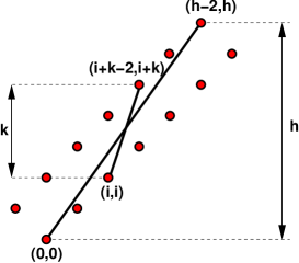
Figure 24. The possible intersections of descending steps of two paths. The first descent is $(h-2,h)\to(0,0)$, and the second is of type $(i+2-k,i+k)\to(i,i)$ with $0\leq k<h$. There are $h-k-1$ possible values of $i$.

Lemma 7.4.

Consider a step of path $\mathcal{P}_{1}$ of type $(h-2,h)\to(0,0)$. Then a descending step of a second path $\mathcal{P}_{2}$ may cross this step only via the following $h(h-1)/2$ possible steps:

$$(i+k-2,i+k)\to(i,i),\qquad{\rm for}\ \ 0\leq i\leq h-k-1,\ \ 0\leq k\leq h-1.$$

A generic case is represented in Fig.24.

7.2.3. A weight preserving involution on families of paths

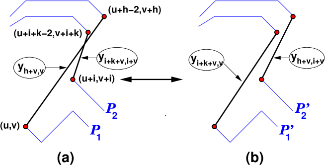
Figure 25. A typical edge intersection of $\Gamma_{\mathbf{M}}$-paths (a) and the result of the flipping operation on it (b). We have the weights of the steps. We have the identity of path weights, since $y_{h+v,v}y_{i+k+v,i+v}=y_{h+v,i+v}y_{i+k+v,v}$. The paths in (b) are said to be “too close” to each other.

Given the list of edge intersections in Lemma 7.4, we define a weight-preserving involution on families of paths which we call flipping. Suppose two paths, $\mathcal{P}_{1}$ and $\mathcal{P}_{2}$, intersect along an edge $e_{1}=(u+h-2,v+h)\to(u,v)$ of $\mathcal{P}_{1}$ and $e_{2}=(u+i+k-2,v+i+k)\to(u+i,v+i)$ of $\mathcal{P}_{2}$. Suppose $\mathcal{P}_{i}=L_{i}\cup e_{i}\cup R_{i}$ ($i=1,2$), where $L_{i}$ is the subpath of $\mathcal{P}_{i}$ before the vertex $(u+h-2,v+h)$, and so forth.

Definition 7.5.

The flipping of $\mathcal{P}_{1}$ and $\mathcal{P}_{2}$ w.r.t. the intersection along the edges $e_{1}$ and $e_{2}$ the configuration of two new paths $\mathcal{P}_{1}^{\prime},\mathcal{P}_{2}^{\prime}$ such that $\mathcal{P}_{i}^{\prime}=L_{i}\cup e_{i}^{\prime}\cup R_{i}$, where $e_{2}^{\prime}=(u+i+k-2,v+i+k)\to(u,v)$ and $e_{1}^{\prime}=(u+h-2,v+h)\to(u+i,v+i)$.

Flipping is illustrated in Figure 25. The weight of two paths $(\mathcal{P}_{1},\mathcal{P}_{2})$ is equal to the product of the weights of $\mathcal{P}_{1}$ and $\mathcal{P}_{2}$.

Lemma 7.6.

The weight of the two paths $(\mathcal{P}_{1},\mathcal{P}_{2})$ is equal to that of the flipped paths $(\mathcal{P}_{1}^{\prime},\mathcal{P}_{2}^{\prime})$ of Definition 7.5.

Proof.

$$w(e_{1})w(e_{2})=y_{h+v,v}y_{i+k+v,i+v}=y_{h+v,i+v}y_{i+k+v,v}=w(e_{i}^{\prime})w(e_{2}^{\prime}),$$

By virtue of Equation (5.4). The rest of the weights of the path configurations are unchanged by the flipping operation, so the Lemma follows. ∎

For the graph $\Gamma_{\mathbf{M}}$, there is a finite list of all possible results of the flipping procedure.

Lemma 7.7.

Given $\Gamma_{\mathbf{M}}$, the results of flipping an intersection between a pair of paths is a pair of paths which include pairs of steps of the form $((u+h-2,v+h)\to(u+i,v+i),(u+j-2,v+j)\to(u,v))$ for any $1\leq i\leq j<h$, where there is a descending edge $v+h\to v$ in $\Gamma_{\mathbf{M}}$.

Proof.

By construction of $\Gamma_{\mathbf{M}}$ (see Section 5.2.1), if there exists a descending edge $v+h\to v$ on $\Gamma_{\mathbf{M}}$, then for all $1\leq i\leq j<h$, the edges $v+j\to v+i$ exist on $\Gamma_{\mathbf{M}}$, as well as $v+h\to v+i$ and $v+j\to v$. The list of the definition therefore exhausts all possible cases of flippings of intersections along edges. ∎

Definition 7.8.

Two paths obtained as the result of the flipping of an intersection are called “too close” to each other.

For example, the paths in Figure 25 (b) are too close.

Conversely, we may define the flipping of a pair of paths which are too close to each other (with respect to the pair of edges that are too close) as the inverse of the transformation of Definition 7.5. The flipping thus defined is an involution.

Definition 7.9.

Two paths are said to be strongly non-intersecting if (i) they do not intersect and (ii) they are not too close.

7.2.4. Generalization of LGV

We have the formula

(7.3) $${R_{{\alpha},n+m_{1}}\over(R_{1,m_{1}})^{\alpha}}=\det_{1\leq i,j\leq{\alpha}}\left({R_{1,n+m_{1}+{\alpha}+1-i-j}\over R_{1,m_{1}}}\right)$$

where $n+m_{1}\geq{\alpha}-1$. Using Theorem 6.13 and the path presentation above, $R_{1,n+m_{1}+{\alpha}+1-i-j}/R_{1,m_{1}}$ is the sum over weighted $\Gamma_{\mathbf{M}}$-paths from $A_{i}=(2i-2,0)$ to $E_{j}=(2n+2{\alpha}-2j,0)$.

The proof of the LGV formula (7.1) uses an involution on configurations of paths, which leaves their weight invariant up to a sign. This cancels various pairs of intersecting paths in the determinant expansion. This involution is defined as follows: it leaves non-intersecting configurations invariant, otherwise, it interchanges the beginnings (until the first intersection) of the two leftmost paths that intersect first. The only terms not cancelled in the determinant correspond to the non-intersecting path configurations.

The determinant (7.3) is also as a sum over families of paths from $\{A_{i}\}_{i=1}^{\alpha}$ to the $\{E_{j}\}_{j=1}^{\alpha}$, with their weight multiplied by the signature of the permutation $\sigma$ such that $A_{i}$ is connected to $E_{\sigma(i)}$.

We define an involution $\Phi$ as follows. If a configuration has at least one intersection or edges which are too close to each other, then $\Phi$ “flips” the beginnings of the two leftmost paths which intersect or are too-close, whichever comes first. That is, we either interchange the beginnings of paths if there is an intersection along a common vertex, or we apply the flipping procedure described above. Configurations which have no intersections nor edges which are too close to each other are invariant under $\Phi$.

The map $\Phi$ is clearly an involution. Applying Lemma 7.6, the total weight of a flipped configuration is invariant. As for the ordinary case, $\Phi$ pairs up terms in the expansion of the determinant which cancel each other, and we are left only with the $\Phi$-invariant configurations. Therefore the determinant (7.3) is equal to the partition function of strongly non-intersecting paths of Definition 7.9.

Theorem 7.10.

For any Motzkin path ${\mathbf{M}}$, and for $n+m_{1}\geq{\alpha}-1$, $R_{{\alpha},n+m_{1}}/(R_{1,m_{1}})^{\alpha}$ is the partition function of configurations of ${\alpha}$ strongly non-intersecting paths on $\Gamma_{\mathbf{M}}$ starting at the points $A_{i}=(2i-2,0)$, $i=1,2,...,{\alpha}$ and ending at the points $E_{j}=(2n+2{\alpha}-2j,0)$, $j=1,2,...,{\alpha}$. The weights are expressed in terms of the Motzkin path as in Theorem 6.7, and (5.5).

7.3. Positivity of $R_{{\alpha},n}$ for all ${\alpha},n$

Theorem 7.10 implies that $R_{{\alpha},n+m_{1}}$ is a positive Laurent polynomial of any initial data, provided $n+m_{1}\geq{\alpha}-1$, since all the weights in Theorem 6.7 and (5.5) are positive Laurent monomials of the initial data ${\mathbf{x}}_{\mathbf{M}}$.

We now consider the case when $n+m_{1}<{\alpha}-1$. The determinant in eq.(7.3) involves some quantities $R_{1,m}$ with indices $m<0$, for which we have no interpretation as partition functions for paths. In order to generalize the result for arbitrary $n\in{\mathbb{Z}}$, we relate the expressions $R_{{\alpha},n+m_{1}}$ in the range $n+m_{1}<{\alpha}-1$ to some expressions $R_{{\alpha}^{\prime},n^{\prime}+m_{1}^{\prime}}$ with $n^{\prime}+m_{1}^{\prime}\geq{\alpha}^{\prime}-1$.

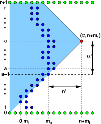
Figure 26. The generic situation $m_{\alpha}+1<n<{\alpha}-1$ in the $(m,{\alpha})$ plane. We have represented the light-cone of values determining $R_{{\alpha},n+m_{1}}$ (shaded area inside the wedge on the left of the point $({\alpha},n+m_{1})$), as well as the initial data, in the form of two parallel Motzkin paths ${\mathbf{M}}=\{(m_{\beta},\beta)\}_{\beta=1}^{r}$ and $\{(m_{\beta}+1,\beta)\}_{\beta=1}^{r}$. The light-cone cuts out a portion ${\mathbf{M}}^{\prime}=\{(m_{\beta},\beta)\}_{\beta=a}^{r}$ of ${\mathbf{M}}$ so that $R_{{\alpha},n+m_{1}}$ only depends on the corresponding initial data. We may therefore truncate the picture by taking as new origin the (dashed) line $\beta=a-1$, and interpret $R_{{\alpha},n+m_{1}}$ as the solution $R_{{\alpha}^{\prime},n^{\prime}+m_{a}}$ of the $A_{r-a+1}$ $Q$-system, with initial data indexed by ${\mathbf{M}}^{\prime}$, and with ${\alpha}^{\prime}={\alpha}-a+1$ and $n^{\prime}=n+m_{1}-m_{a}$.

Consider the case when $m_{\alpha}+1<n+m_{1}<{\alpha}-1$. Due to the structure of the $Q$-system, each $R_{\beta,n}$ is inductively obtained from the values $R_{\beta,n-1}$, $R_{\beta,n-2}$, $R_{\beta+1,n-1}$ and $R_{\beta-1,n-1}$. Consequently, $R_{{\alpha},n+m_{1}}$ is a function only of the initial data that are contained in a “light-cone” of values of $(\beta,m)$, such that ${\alpha}-n-m_{1}+k\leq\beta\leq{\alpha}+n+m_{1}-k$, for $k<n+m_{1}$ (see Fig.26).

In fact, $R_{{\alpha},n+m_{1}}$ depends only on the initial data ${\mathbf{x}}_{{\mathbf{M}}^{\prime}}$ corresponding to a subset ${\mathbf{M}}^{\prime}=\{(m_{\alpha},{\alpha})\}_{{\alpha}=a}^{r}$ of the Motzkin path ${\mathbf{M}}$, namely such that $(a,m_{a}+1)$ lies on the boundary of the light-cone, i.e. $a={\alpha}-n-m_{1}+k$ and $m_{a}+1=k$. For the sake of this calculation we may freely modify the values of $R_{a-1,m}$ and set them to $1$, as they are not involved in the expression of $R_{{\alpha},n+m_{1}}$. This has the effect of transforming the problem into one for $A_{r^{\prime}}$, with $r^{\prime}=r-a+1$.

More precisely, $R_{{\alpha},n+m_{1}}$, as a function of a subset of the initial data ${\mathbf{x}}_{\mathbf{M}}$, may be reinterpreted as the solution $R_{{\alpha}^{\prime},n^{\prime}+m_{1}^{\prime}}^{\prime}$ of the $A_{r^{\prime}}$ $Q$-system, expressed in terms of the initial data ${\mathbf{x}}_{{\mathbf{M}}^{\prime}}$, with $m_{\beta}^{\prime}=m_{a+\beta-1}$, $\beta=1,2,..,r-a+1$. In this new expression, we have $n^{\prime}+m_{1}^{\prime}=n+m_{1}={\alpha}-a+m_{a}+1={\alpha}^{\prime}+m_{a}\geq{\alpha}^{\prime}$.

Note that the minimum $m^{\prime}$ of $m_{\beta}$ on the interval $[a,r]$ may be strictly positive. In that case, we must use the translational invariance property of Lemma 2.3 (see also eq.(2.4)) to first translate both the Motzkin path ${\mathbf{M}}^{\prime}$ and the index $n^{\prime}$ by $-m^{\prime}$. We get $n^{\prime}-m^{\prime}+m_{1}^{\prime}={\alpha}^{\prime}+m_{1}^{\prime}-m^{\prime}\geq{\alpha}^{\prime}$, and the Theorem 7.10 can be applied to conclude that $R_{{\alpha}^{\prime},n^{\prime}-m^{\prime}+m_{1}^{\prime}}^{\prime}$ is a positive Laurent polynomial of the translated initial data ${\mathbf{x}}_{{\mathbf{M}}^{\prime\prime}}$ corresponding to $m_{\beta}"=m_{\beta}^{\prime}-m^{\prime}$ for all $\beta$. By Lemma 2.3, we find that $R_{{\alpha}^{\prime},n^{\prime}+m_{1}^{\prime}}^{\prime}$ is a positive Laurent polynomial of the un-translated data ${\mathbf{x}}_{{\mathbf{M}}^{\prime}}$.

We deduce that $R_{{\alpha},n}$ is a positive Laurent polynomial of the initial data ${\mathbf{x}}_{\mathbf{M}}$ for all values of $n>m_{\alpha}+1$.

Finally, the positivity result is extended to $n<m_{\alpha}$ (including negative values of $n$) by use of the corresponding invariance $n\to-n$ of the $Q$-system (see Lemma 2.1), and the same trick as in the proof of Theorem 6.13, involving the reflected-translated Motzkin path ${\mathbf{M}}^{\prime}$. We deduce the final:

Theorem 7.11.

The solution $R_{{\alpha},n}$ of the $Q$-system for $A_{r}$ is a Laurent polynomial with non-negative integer coefficients of any initial data ${\mathbf{x}}_{\mathbf{M}}$ indexed by any Motzkin path ${\mathbf{M}}$, for all $n\in{\mathbb{Z}}$.

8. Asymptotics

In this section, we consider two limiting cases of the results: Solutions in the the limit $r\to\infty$, corresponding to the $Q$-sytem of $A_{\infty/2}$, and solutions $R_{1,n}$ when $n\to\infty$. In the latter case, we are interested in the asymptotic behavior of the number of paths contributing to the partition function $R_{1,n}$ as $n\to\infty$.

8.1. The limit $A_{\infty/2}$

In Equation (1.4), retaining only the boundary condition at ${\alpha}=0$, $R_{0,n}=1$ ($n\in{\mathbb{Z}}$) but dropping the condition at ${\alpha}=r+1$, gives us the solutions for the algebra $A_{\infty/2}$. All of the results of the previous sections generalize in a straightforward way.

The initial seed is an infinite sequence, $(R_{{\alpha},m_{\alpha}},R_{{\alpha},m_{\alpha}+1})_{{\alpha}\in{\mathbb{Z}}_{+}}$ indexed by semi-infinite Motzkin paths ${\mathbf{M}}$. For example, for ${\mathbf{M}}_{0}=(0,0,...)$, and the corresponding heap graph is $G_{\infty/2}$, generalizing Figure 6. Then $R_{1,n}$ as a function of ${\mathbf{x}}_{{\mathbf{M}}_{0}}$ is $R_{1,0}$ times the generating function for weighted heaps on $G_{\infty/2}$, $F_{1}(t)$ obtained as the limit of (4.4):

(8.1) $$F_{1}(t)=1+t{y_{1}\over 1-ty_{1}-t{y_{2}\over 1-ty_{3}-t{y_{4}\over 1-ty_{5}-t{y_{6}\over{}\ \ {\ddots\over 1-ty_{2{\alpha}-1}-t{y_{2{\alpha}}\over{}\ \ \ \ddots}}}}}}$$

Using the rearrangement Lemmas 4.5 and 4.6 we can write the expressions for the generating function in terms of other initial seeds. For instance, the generating function corresponding to the “maximal” Motzkin path ${\mathbf{M}}_{\max}$ with $m_{\alpha}={\alpha}-1$ is the continued fraction:

(8.2) $${1\over 1-t{y_{1}\over 1-t{y_{2}\over 1-t{y_{3}\over 1-t{y_{4}\over 1-t{y_{5}\over 1-t{y_{6}\over{}\ \ {\ddots\over 1-t{y_{{\alpha}}\over{}\ \ \ \ddots}}}}}}}}}$$

The limit of the generating function corresponding to the strictly descending Motzkin path with $r$ vertices, of the form $1/(1-ty_{1}\varphi_{r})$, with $\varphi_{r}$ as in Lemma 6.2 is a “continued fraction” with infinitely many branchings, a sort of self-similar object.

8.2. Numbers of configurations

We consider the number of configurations contributing to $R_{1,n}$ in general. For this purpose, set $R_{{\alpha},m_{\alpha}}=R_{{\alpha},m_{{\alpha}+1}}=1$ (${\alpha}=1,2,...,r$). This implies that all the edge weights are $y_{e}=1$. Therefore, $R_{{\alpha},n}$ is a non-negative integer equal counts the numbers of configurations of the related statistical model.

For example, when ${\mathbf{M}}={\mathbf{M}}_{0}$,

Lemma 8.1.

For the initial data $R_{{\alpha},0}=R_{{\alpha},1}=1$, ${\alpha}=1,2,...,r$, the generating function $F_{1}^{(r)}(t)=\sum_{n\geq 0}R_{1,n}t^{n}$ reads:

(8.3) $$F_{1}^{(r)}(t)=1+t{P_{r}(t)\over P_{r+1}(t)},\ {\rm with}\ \ P_{m}(t)=t^{m\over 2}U_{m}\left({1\over\sqrt{t}}-\sqrt{t}\right)$$

where $U_{m}$ are the Chebyshev polynomials of the second kind, with $U_{m}(2\cos\theta)={\sin(m+1)\theta\over\sin\theta}$. The corresponding limit $r\to\infty$ for $A_{\infty/2}$ reads:

(8.4) $$F_{1}^{(\infty)}(t)=1+tz(t)={3-t-\sqrt{1-6t+t^{2}}\over 2}=1+t+2t^{2}+6t^{3}+22t^{4}+90t^{5}+394t^{6}+\cdots$$

where $z(t)={1-t-\sqrt{1-6t+t^{2}}\over 2t}$ is the generating function of the large Schroeder numbers.

Proof.

We use the expression (4.4) with all weights equal to 1. Then there is a recursion relation, $P_{r+1}(t)=(1-t)P_{r}(t)-tP_{r-1}(t)$, with $P_{0}(t)=1$ and $P_{1}(t)=1-t$. The limit $z(t):=\lim_{r\to\infty}P_{r}(t)/P_{r+1}(t)$ therefore satisfies $z=1-t+{t\over z}$. It also coincides with the continued fraction (8.1) with $y_{i}=1$ for all $i$. ∎

The rate of growth of $R_{1,n}$, considered as the number of paths of length $2n$ on $\Gamma_{{\mathbf{M}}_{0}}$, can also be analyzed. The radius of convergence of the series $F_{1}^{(r)}(t)$ is given by the smallest root of the denominator of the fraction, which is $U_{r+1}\big{(}{1\over\sqrt{t}}-\sqrt{t}\big{)}$. As the zeros of the Chebyshev polynomial $U_{m}$ are $2\cos\,\pi{k\over m+1}$, $k=1,2,...,m$, when $n\to\infty$

(8.5) $$R_{1,n}\sim C_{r}\times\left(\cos\big{(}{\pi\over r+2}\big{)}+\sqrt{\cos^{2}\big{(}{\pi\over r+2}\big{)}+1}\right)^{2n}$$

for some constant $C_{r}$.

The number of paths on $\Gamma_{{\mathbf{M}}_{max}}$ is also simple to compute, as it is the number of Dyck paths of length $2n$, which are limited by height $2r+1$:

(8.6) $$F_{1}^{(r)}(t)={1\over\sqrt{t}}{U_{2r+1}\left({1\over\sqrt{t}}\right)\over U_{2r+2}\left({1\over\sqrt{t}}\right)}$$

In the limit $r\to\infty$,

(8.7) $$F_{1}^{(\infty)}(t)={1-\sqrt{1-4t}\over 2t}=1+t+2t^{2}+5t^{3}+14t^{4}+42t^{5}+429t^{6}+\cdots$$

is the generating function of the Catalan numbers $c_{n}={1\over n+1}{2n\choose n}$.

As a result of the correspondence to domino tilings in the next section, this function counts the number of domino tilings of the (possibly truncated) halved Aztec diamond with $d$ tiles missing. The function $R_{{\alpha},n}$ counts the number of its indented versions.

The large $n$ behavior is $R_{1,n}\sim C_{r}^{\prime}\big{(}2\cos({\pi\over 2r+3})\big{)}^{2n}$, for some constant $C_{r}^{\prime}$.

Now consider the expression as a function of the initial seed corresponding to ${\mathbf{M}}_{2}$, with $m_{\alpha}=r-{\alpha}$ (the maximal descending Motzkin path), where $R_{1,n+r-1}/R_{1,r-1}$ is as in Lemma 6.2.

$$F_{1}^{(r)}(t)=\sum_{j=0}^{r-2}R_{1,j}t^{j}+t^{r-1}R_{1,r-1}\Phi_{r}(t;{\mathbf{y}}),\qquad\Phi_{r}(t;{\mathbf{y}})={1\over 1-ty_{1}\varphi_{r}(\{y_{j}\};\{y_{i,j}\};c)},$$

where $\varphi_{r}$ is defined in Lemma 6.2, and the arguments are the weights $y_{i}=y_{i}({\mathbf{M}}_{2})$, $i=2,3,...,2r$, $y_{i,j}=y_{i,j}({\mathbf{M}}_{2})$, $2\leq j+1<i\leq r+1$, and $c=ty_{2r+1}({\mathbf{M}}_{2})$.

Lemma 8.2.

Setting $R_{{\alpha},r-{\alpha}}=R_{{\alpha},r-{\alpha}+1}=1$ (${\alpha}\in I_{r}$),

(8.8) $$\Phi_{r}(t)=1+t{V_{r}(t)\over V_{r+1}(t)},\ \ V_{m}(t)=(-1)^{m}U_{2m}(\sqrt{t}).$$

Proof.

Setting the weights $y$’s to $1$ in $1/(1-t\varphi_{r})$, using the recursive definition of $\varphi_{r}$ of Lemma 6.2 with $\varphi_{m}(\{y_{j}\};\{y_{i,j}\};ty_{2m+1})|_{{\mathbf{y}}=1}={1\over 1-\theta_{m}(t)}$ ($m\geq 0$), $\varphi_{0}=1$ and $\theta_{0}=0$, we have $\theta_{m}={t+\theta_{m-1}\over 1-t-\theta_{m-1}}$. Let $1-t-\theta_{m}={V_{m+1}\over V_{m}}$, then we have a three-term recursion relation for $V_{m}$: $V_{m+1}=(2-t)V_{m}-V_{m-1}$, where $V_{0}=1,V_{1}=1-t$ (or equivalently $V_{-1}=V_{0}=1$). The solution is $V_{m}(t)=(-1)^{m}U_{2m}(\sqrt{t})$, by iterating the Chebyshev recursion relation $U_{m+1}(x)=xU_{m}(x)-U_{m-1}(x)$, to get $U_{n+1}=(x^{2}-2)U_{n-1}-U_{n-3}$, and identifying the initial conditions. ∎

The asymptotic behavior of $R_{1,n}$ with these boundary conditions is found from the smallest root of the denominator $U_{2r+2}(\sqrt{t})$. Then

(8.9) $$R_{1,n}\sim C_{r}^{\prime\prime}\times{1\over\left(2\sin\big{(}{\pi\over 2(2r+3)}\big{)}\right)^{2n}}$$

as $n\to\infty$, for some constant $C_{r}^{\prime\prime}$.

In this case, the limit $r\to\infty$ of $\Phi_{r}$ is ill-defined. The Motzkin path ${\mathbf{M}}_{2}$ has $m_{1}=r-1\to\infty$, hence does not have a good limit in our picture. More importantly, the graph $\Gamma_{{\mathbf{M}}_{2}}$ has an infinite number of incoming edges at each vertex $1,2,3...$. Hence, as we count paths according to their numbers $n$ of down steps, we get an infinite number of paths from $0$ to $0$ as soon as $n\geq 2$. This can also be seen in the fact that the rate of growth in eq.(8.9) diverges as $2r/\pi$.

Example 8.3.

In the cases $r=1,2,3$, we have

$$\Phi_{1}(t) = {1\over 1-{t\over 1-{t\over 1-t}}}=1+t{1-t\over 1-3t+t^{2}}=1-t{U_{2}(\sqrt{t})\over U_{4}(\sqrt{t})}$$

$$\Phi_{2}(t) = {1\over 1-{t\over 1-{t+{t\over 1-t}\over 1-t-{t\over 1-t}}}}=1+t{1-3t+t^{2}\over 1-6t+5t^{2}-t^{3}}=1-t{U_{4}(\sqrt{t})\over U_{6}(\sqrt{t})}$$

$$\Phi_{3}(t) = {1\over 1-{t\over 1-{t+{t+{t\over 1-t}\over 1-t-{t\over 1-t}}\over 1-t-{t+{t\over 1-t}\over 1-t-{t\over 1-t}}}}}=1+t{1-6t+5t^{2}-t^{3}\over 1-10t+15t^{2}-7t^{3}+t^{4}}=1-t{U_{6}(\sqrt{t})\over U_{8}(\sqrt{t})}$$

More generally, for arbitrary choices of ${\mathbf{M}}$ and the associated initial conditions $R_{{\alpha},m_{\alpha}}=R_{{\alpha},m_{\alpha}+1}=1$, we have $F_{1}^{(r)}(t)=L_{r}(t)/K_{r+1}(t)$, where $L_{m}(t),K_{m}(t)$ are polynomials of degree $m$ with integer coefficients depending on ${\mathbf{M}}$, and $K_{m}(0)=1$ and $K_{m}(t)\sim(-t)^{m}$ for large $t$. Indeed, from the results of Section 3, we know that $K_{r+1}(t)$ is the generating function for hard particles on $G_{\mathbf{M}}$, with weight $-t$ per particle. So the empty configuration contributes $K_{r+1}(0)=1$. Due to connectivity of $G_{\mathbf{M}}$, the maximally occupied hard-particle configuration corresponds to all odd vertices $2i+1$, $i=0,1,...,r$ being occupied by a particle (these are the duals of all the skeleton-tree edges of $\Gamma_{\mathbf{M}}$, with odd labels). The corresponding weight is therefore $(-t)^{r+1}$.

For $r$ large, it is always possible to reexpress $F_{1}^{(r)}(t)$ for any Motzkin path ${\mathbf{M}}$ obtained from ${\mathbf{M}}_{0}$ via finitely many mutations in the form of a rational fraction of the variables $t$ and $P_{r-1}(t)/P_{r}(t)$. Indeed, the branchings of the continued fraction expression for $F_{1}^{(r)}(t)$ all include some “tails” of the form $1/(1-ty_{a}-t(y_{b}/(1-ty_{c}...)))$ which, when we set all $y_{i}=1$, reduce to some ratio $P_{m}(t)/P_{m+1}(t)$. By use of the 3-term recursion relation for $P_{m}$, this can always be rewritten as a rational fraction of $t$ and $P_{r-1}/P_{r}$. Then, in the case of $A_{\infty/2}$, upon taking the limit $r\to\infty$, we see that, as $P_{r-1}/P_{r}\to z(t)$, $F_{1}^{(r)}(t)$ takes the general form $A(t)+B(t)\sqrt{1-6t+t^{2}}$, where $A$ and $B$ are rational fractions of $t$ with integer coefficients.

For instance let us take ${\mathbf{M}}=\mu_{1}{\mathbf{M}}_{0}$. Then we have

$$F_{1}^{(r)}(t) = R_{1,0}+{tR_{1,1}\over 1-t{y_{1}\over 1-t{y_{2}+{y_{3,1}\over 1-ty_{5}-t{y_{6}\over 1-ty_{7}-\cdots}}\over 1-ty_{3}-t{y_{4}\over 1-ty_{5}-t{y_{6}\over 1-ty_{7}-\cdots}}}}}\Bigg{|}_{{\mathbf{y}}=\bf 1}$$

$$= 2+{t\over 1-{t\over 1-t\left(1+{P_{r-2}(t)\over P_{r-1}(t)}\right){P_{r-1}(t)\over P_{r}(t)}}}=2+t+{t^{2}\over 2-t-{P_{r-1}(t)\over P_{r}(t)}}$$

where we have used the $Q$-system to rewrite $R_{1,0}={R_{1,1}^{2}+R_{2,1}\over R_{1,2}}=2$, and the recursion relation for $P$ to eliminate $P_{r-2}$. In the limit $r\to\infty$, this yields for the $A_{\infty/2}$ $Q$-system with initial conditions $R_{1,1}=R_{1,2}=1$ and $R_{{\alpha},0}=R_{{\alpha},1}=1$ for all ${\alpha}\geq 2$:

$$F_{1}^{(\infty)}(t)=2+t+{t^{2}\over 2-t-z(t)}=2+t+t^{2}{1-5t+2t^{2}+\sqrt{1-6t+t^{2}}\over 1-7t+5t^{2}-t^{3}}$$

9. The relation to domino tilings

The solutions of the $A_{\infty}$ $T$-system, also known as the octahedron equation [21, 10, 17],

(9.1) $$T_{i,j,k+1}T_{i,j,k-1}=T_{i,j+1,k}T_{i,j-1,k}-T_{i+1,j,k}T_{i-1,j,k}$$

were given in [22] in terms of the partition function for domino tilings of the Aztec diamond and its generalizations. The $A_{r}$ $T$-system (the same equation, with additional boundary conditions) is the fusion relation satisfied by the transfer matrix of the generalized, inhomogeneous Heisenberg spin chain [15]. The $Q$-system (1.1) is a limit of the $T$-system, with the index $j$ dropped, whereas the renormalized $Q$-system (1.4) is obtained by formally dropping the index $i$. Therefore one should be able to recover the solutions of the $Q$-system from those of the $T$-system.

Here, we give the explicit connection between the path formulation of $R_{{\alpha},n}$ and domino tilings. In particular, we express $R_{{\alpha},n}({\mathbf{x}}_{\mathbf{M}})$ for any Motzkin path ${\mathbf{M}}$, as partition functions for tilings of certain domains of the square lattice by means of $2\times 1$ and $1\times 2$ dominos, and of rigid “defect” pairs of square tiles $1\times 1$.

9.1. Paths and matchings of the Aztec diamond

In this subsection, we consider the solutions $R_{{\alpha},n}$ as functions of ${\mathbf{x}}_{0}.$ For a restricted subset of the indices $({\alpha},n)$ there is an alternative combinatorial interpretation of $R_{{\alpha},n}$, related to the results of [22] on the solutions of the octahedron equation. This relation holds only for a restricted subset, because the boundary conditions of [22] are incompatible with our truncation $R_{0,n}=R_{r+1,n}=1$. The connection is therefore valid only sufficiently far away from these boundaries.

Consider a system of equations with indices $({\alpha},n)\in{\mathbb{Z}}\times{\mathbb{Z}}$ (the $A_{\infty}$ $Q$-system):

(9.2) $$\rho_{{\alpha},n+1}\rho_{{\alpha},n-1}=\rho_{{\alpha},n}^{2}+\rho_{{\alpha}+1,n}\rho_{{\alpha}-1,n},\ {\alpha},n\in{\mathbb{Z}}$$

To write $\rho_{{\alpha},n}$ as a function of $\{\rho_{{\alpha},0},\rho_{{\alpha},1}\}_{{\alpha}\in{\mathbb{Z}}}$ we use the recursion relation

$$\rho_{{\alpha},n+1}={\rho_{{\alpha},n}^{2}+\rho_{{\alpha}+1,n}\rho_{{\alpha}-1,n}\over\rho_{{\alpha},n-1}}.$$

By induction, $\rho_{{\alpha},n}$ depends only on the subset of the initial data $\{\rho_{\beta,0},\rho_{\beta,1}\}$ with ${\alpha}-n+1\leq\beta\leq{\alpha}+n-1$. Hence, if we identify $\rho_{{\alpha},i}=R_{{\alpha},i}$ ($i=0,1$), then $\rho_{{\alpha},n}=R_{{\alpha},n}$ if

(9.3) $$n\leq{\rm Min}({\alpha},r+1-{\alpha}).$$

We will show that $R_{{\alpha},n}$, with indices in the set, is the generating function for positively weighted matchings of the Aztec diamond.

Recall the interpretation of $\rho_{{\alpha},n}$ in terms of partition functions of matchings of Aztec diamonds [22]. The Aztec diamond centered at $({\alpha},0)$ of radius $n$ is the set ${\mathcal{A}}_{{\alpha},n}=\left\{(\beta,\gamma)\in{\mathbb{Z}}^{2},\,|\,|{\alpha}-\beta|+|\gamma|<n\right\}$ with boundary ${\mathcal{B}}_{{\alpha},n}=\left\{(\beta,\gamma)\in{\mathbb{Z}}^{2},\,|\,|{\alpha}-\beta|+|\gamma|=n\right\}$ We denote by $A_{{\alpha},n}$ and $B_{{\alpha},n}$ the subsets of the square lattice with vertices in ${\mathbb{Z}}^{2}+({1\over 2},{1\over 2})$ made of squares centered on the points of ${\mathcal{A}}_{{\alpha},n}$ and ${\mathcal{B}}_{{\alpha},n}$ respectively.

Consider the matchings, or compact dimer coverings, of $A_{{\alpha},n}$. These are configurations of occupation of edges (including their vertices) of $A_{{\alpha},n}$ by dimers, where each vertex is covered by exactly one dimer. Each square $(\beta,\gamma)\in A_{{\alpha},n}$ has either 2,1, or 0 edges covered, and we define $\epsilon(\beta,\gamma)=-1,0,1$, respectively. Each square $(\beta,\gamma)\in B_{{\alpha},n}$ has either $0$ or $1$ edge covered, and we define $\epsilon(\beta,\gamma)=0,1$ respectively. Let

$$\theta_{{\alpha},n}(\beta,\gamma)=\left\{\begin{matrix}0&{\rm if}\,{\alpha}+\beta+\gamma+n=0\,{\rm mod}\,2\\ 1&{\rm otherwise}\end{matrix}\right.$$

Then the generating function for matchings of $A_{{\alpha},n}$ is

(9.4) $$M_{{\alpha},n}=\sum_{{\rm matchings}\,{\rm of}\,A_{{\alpha},n}}\prod_{(\beta,\gamma)\in{\mathcal{A}}_{{\alpha},n}\cup{\mathcal{B}}_{{\alpha},n}}\Big{(}\rho_{\beta,\theta_{{\alpha},n}(\beta,\gamma)}\Big{)}^{\epsilon(\beta,\gamma)}.$$

The following is proved in [22]:

Theorem 9.1.

The solution $\rho_{{\alpha},n}$ of the system (9.2), expressed as a function of $\{\rho_{{\alpha},0},\rho_{{\alpha},1}\}_{{\alpha}\in{\mathbb{Z}}}$, is equal to the generating function for matchings of $A_{{\alpha},n}$ (9.4).

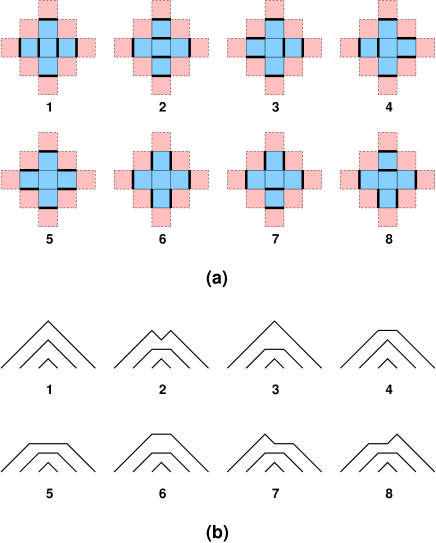
Figure 27. (a) The $8$ matchings of $A_{{\alpha},3}$ and (b) the non-intersecting $G_{r}$-paths from $(0,0),(2,0),(4,0)$ to $(6,0),(8,0),(10,0)$, where $r\geq 4$. The labeling corresponds to the weights $a_{i}$, $i=1,2,...,8$.

Example 9.2.

Figure 27 shows, for $n=3$, (a) the eight matchings of the Aztec diamond $A_{{\alpha},3}$, centered at $({\alpha},0)$ after rotation by $\pi/4$. The corresponding weights of eq.(9.4) are (we denote by $a_{i}$ the weight of the configuration labeled $i$ in Fig.27):

$$a_{1}={R_{{\alpha}-2,1}R_{{\alpha},1}R_{{\alpha}+2,1}\over R_{{\alpha}-1,0}R_{{\alpha}+1,0}},\ \ a_{2}={R_{{\alpha}-1,1}^{2}R_{{\alpha}+1,1}^{2}\over R_{{\alpha},0}^{2}R_{{\alpha},1}},\ \ a_{3}={R_{{\alpha}-1,1}^{2}R_{{\alpha}+2,1}\over R_{{\alpha}-1,0}R_{{\alpha}+1,0}},$$

$$a_{4}={R_{{\alpha}-2,1}R_{{\alpha}+1,1}^{2}\over R_{{\alpha}-1,0}R_{{\alpha}+1,0}},\ \ a_{5}={R_{{\alpha},1}^{3}\over R_{{\alpha},0}^{2}},\ \ a_{6}={R_{{\alpha}-1,1}^{2}R_{{\alpha}+1,1}^{2}\over R_{{\alpha}-1,0}R_{{\alpha},0}R_{{\alpha}+1,0}},\ \ a_{7}=a_{8}={R_{{\alpha}-1,1}R_{{\alpha},1}R_{{\alpha}+1,1}\over R_{{\alpha},0}^{2}}$$

and we have $R_{{\alpha},3}=\sum_{i=1}^{8}a_{i}$. Note that this expression is valid only for ${\alpha}=2,3,...,r-1$, $r\geq 3$, and provided we set $R_{0,n}=R_{r+1,n}=1$ for all $n$. This can be compared to our previous result for $R_{{\alpha},3}$ as solution of the $A_{r}$ $Q$-system, obtained by cutting out the initial data at $\beta={\alpha}-3$, hence working instead with $A_{r^{\prime}}$, $r^{\prime}=r-{\alpha}+3$. This allows to reinterpret $R_{{\alpha},3}$ for $A_{r}$ as $R_{3,3}^{\prime}$ for $A_{r-{\alpha}+3}$, with initial data $R_{{\alpha}^{\prime},i}^{\prime}=R_{{\alpha}^{\prime}+{\alpha}-3,i}$, $i=0,1$ and ${\alpha}^{\prime}=1,2,...,r-{\alpha}+3$. As such it is interpreted as $(R_{{\alpha}-2,0})^{3}$ ($=(R_{1,0}^{\prime})^{3}$) times the generating function for triples of non-intersecting $G_{r}$-paths (for any $r\geq 4$) from the points $(0,0),(2,0),(4,0)$ to the points $(6,0),(8,0),(10,0)$, but with the weights $y_{1}^{\prime}={R_{{\alpha}-2,1}\over R_{{\alpha}-2,0}}$ and $y_{2\beta-1}^{\prime}={R_{\beta+{\alpha}-3,1}R_{\beta+{\alpha}-4,0}\over R_{\beta+{\alpha}-3,0}R_{\beta+{\alpha}-4,1}}$ for $\beta\geq 2$ and $y_{2\beta}^{\prime}={R_{\beta+{\alpha}-4,0}R_{\beta+{\alpha}-2,1}\over R_{\beta+{\alpha}-3,0}R_{\beta+{\alpha}-3,1}}$ for $\beta\geq 1$. There are exactly $8$ such triples, and their weights (multiplied by $R_{{\alpha}-2,0}^{3}$) match one by one the weights $a_{i}$ above. They are represented in Fig.27 (b).

9.2. Lattice paths and domino tilings

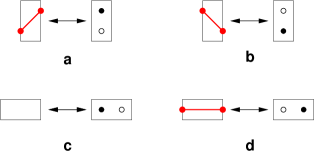
Figure 28. A bijection between lattice paths and domino tilings. The dual square lattice is bicolored, so there are 4 possible domino tiles, labeled $a,b,c,d$. Each corresponds to a step of path as indicated: $a:(1,1)$, $b:(1,-1)$, $c:$ no step, and $d:(2,0)=(1,0)+(1,0)$, double horizontal step.

There is a standard bijection between domino tilings and $\widetilde{G}_{r}$ lattice paths. (see e.g. [13]). Consider the dominos as tiling a chessboard. Then there are four types of $2\times 1$ or $1\times 2$ dominos (see Figure 28). These are in bijection with the four path steps: $(1,1)$, $(1,-1)$, $(2,0)=(1,0)+(1,0)$ or no step at all. Thus, a domino tiling of a domain $\mathcal{D}$ can be rephrased in terms of a configuration of non-intersecting paths connecting points on the boundary $\partial\mathcal{D}$.

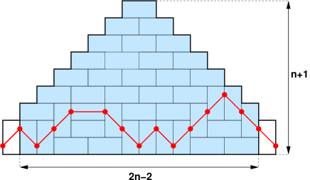
Figure 29. The bijection between paths of length $2n$ steps from $(0,0)$ to $(2n,0)$ and domino tilings of a “halved” Aztec diamond $HA_{n}$, of width $2n$ and height $n+1$.

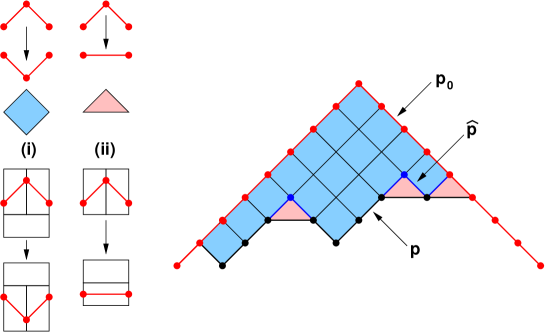
Figure 30. The local moves (i-ii) which give any Aztec path $p$ from the maximal path $p_{0}$, and an example of such a transformation. First one goes from $p_{0}$ to the Dyck path $\hat{p}$ closest to $p$ by a sequence of “box removals” (i), before getting to $p$ via “half-box removals” (ii).

Conversely, consider $\widetilde{G}_{\infty}$-lattice paths in the non-negative integer quadrant ${\mathbb{Z}}_{+}^{2}$ from $(0,0)$ to $(2n,0)$ of length $2n$. (We call these Aztec paths in this section.)

Lemma 9.3.

Aztec paths are in bijection with domino tilings of the “halved” Aztec diamond $HA_{n}$ represented in Figure 29, of width $2n$ and height $n+1$, with a floor at height $h=-1/2$, a ceiling at height $h=n+1/2$, and a white face on the bottom left.

Proof.

Any Aztec path may be obtained from the “maximal” Aztec path $p_{0}$ ($n$ up steps followed by $n$ down steps) using the procedure shown in Figure 30.

Given the path $p_{0}$, use the tiles $a,b,d$ of Figure 28 to tile the region traversed by the path. One must then tile $HA_{n-1}^{\prime}$, the half Aztec diamond below this region, with width $2n-2$ and with the bottom row removed. The bottom left and right corner tiles are frozen, and are of type $c$, as are all the tiles touching the left and right boundaries of $HA_{n-1}^{\prime}$. By induction, the entire domain $HA_{n-1}^{\prime}$ must be tiled with $c$ tiles, a unique configuration. Therefore there is a unique tiling of $HA_{n}$ associated to the maximal path $p_{0}$.

For any other path $p$, we use the sequence of moves in Figure 30, from $p_{0}$ to $p$, and apply the corresponding transformations on the associated tiling by use of the bijection of Fig.28. This produces a unique tiling of $HA_{n}$ for each Aztec path $p$.

Conversely, given any tiling of $HA_{n}$, there is a unique path associated to it via the map in Figure 28. A path can only enter the domain from its lower left end ($1\times 2$ domino of type $a$ or $2\times 1$ domino of type $d$), as all faces touching the left boundary are black, hence the tile $d$ cannot be used. Similarly, the path can only exit via the lower right end ($1\times 2$ domino of type $b$ or $2\times 1$ domino of type $d$). We deduce that there is a unique path associated to the tiling, that goes from $(0,0)$ to $(0,2n)$. ∎

We assign weights to the steps of Aztec paths according to the height $h$ at which the step starts:

• Weight $1$ for steps of type $(1,1)$, irrespectively of $h$.

• Weight $z_{2h-2}$ for a step $(1,-1)$ from height $h$ to $h-1$, $h\geq 2$; weight $z_{1}$ for a step $(1,-1)$ from $h=1$ to $h=0$.

• weight $z_{2h-1}$ for a step $(2,0)$ at height $h$, $h\geq 2$; weights $w_{0},w_{1}$ for steps $(2,0)$ at heights $h=0$ and $h=1$, respectively.

Domino tilings receive weights according to the bijection of Figure 28, with domino $c$ having weight $1$. We will refer to those as weighted domino tilings in the following.

9.3. $Q$-system solutions as functions of ${\mathbf{x}}_{0}$ and domain tilings

Recall the interpretation of $R_{1,n}$ as the partition function of weighted paths on ${\tilde{G}}_{r}$. These are weighted Aztec paths with the following identification of weights: $z_{2r+1}=w_{0}=w_{1}=z_{j}=0$ $(j\geq 2r+3)$, $z_{i}=y_{i}$ $(i=1,2,...,2r)$ and $z_{2r+2}=y_{2r+1}$, with $y_{j}$ as in (3.17). The condition $z_{j}=0$ for $j\geq 2r+4$ corresponds to truncating the tiled domain to the inside of a strip of height $r+3$, with a ceiling at height $h=r+5/2$, with floor at height $h=-1/2$. The conditions $w_{0}=w_{1}=z_{2r+1}=z_{2r+3}=0$ forbid the use of the tile $d$ in the two bottom ($-1/2\leq h\leq 3/2$) and top ($r+1/2\leq h\leq r+5/2$) rows.

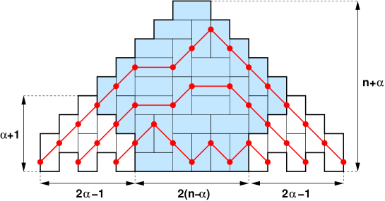
Figure 31. The bijection between families of ${\alpha}$ Aztec paths on ${\mathbb{Z}}_{+}^{2}$ from $(0,0),(2,0),...,(2{\alpha}-2,0)$ to $(2n,0),(2n+2,0),...,2n+2{\alpha}-2,0)$ and the domino tilings of the indented halved Aztec diamond $IHA_{n,{\alpha}}$ of width $2n+2{\alpha}-2$ and height $n+{\alpha}$. Here, ${\alpha}=3$.

Lemma 9.4.

The families of ${\alpha}$ non-intersecting Aztec paths on ${\mathbb{Z}}_{+}^{2}$ from $(0,0),(2,0),...,(2{\alpha}-2,0)$ to $(2n,0),(2n+2,0),...,2n+2{\alpha}-2,0)$, with steps $(1,1)$, $(1,-1)$ and double steps $(2,0)=(1,0)+(1,0)$, are in bijection with domino tilings of the “indented halved” Aztec diamond $IHA_{n,{\alpha}}$ represented in Fig.31.

Proof.

Along the same lines as for the ${\alpha}=1$ case of Lemma 9.3. We first associate a tiling to any configuration of ${\alpha}$ non-intersecting Aztec paths. We simply use the fact that any configuration of ${\alpha}$ non-intersecting Aztec paths may be obtained from the configuration where all paths are maximal via successive applications of the local moves of Fig.30. We apply the construction of the proof of Lemma 9.3 to the bottom-most path, then to the next bottom-most, etc.

Conversely, to construct the path configurations from the tilings, we note that the two successions of ${\alpha}-1$ indentations of the bottom boundary (left and right) impose the presence of ${\alpha}-1$ tiles $a$ and one $a$ or $d$ on the left and ${\alpha}-1$ tiles $b$ and one $b$ or $d$ on the right, and that paths can enter or exit nowhere else on the boundary, due to coloring constraints. This corresponds to exactly ${\alpha}$ paths touching the boundary of the domain, entirely determined by the tiling. ∎

Given that $R_{{\alpha},n}$ is the partition function of ${\alpha}$ non-intersecting Aztec paths, with the identification of weights as above, this gives the relation to domino tilings.

For sufficiently large $r$, the restriction of the weights effectively reduces the domain to be tiled to the shaded region in Figure 31, as the tiling of the rest of the domain is entirely fixed (only dominos $a$ on the left, and $b$ on the right). The case ${\alpha}=1$ is also depicted with the same convention in Fig.29.

In the particular case when ${\alpha}=n$, and $r\geq 2n-1$, the shaded domain to be tiled is exactly the Aztec diamond itself (with width and height $2n-2$), with no constraints. It is interesting to compare the partition function $D_{n}({\mathbf{y}})$ for the weighted tilings of this domain to the partition function for weighted Aztec diamond matchings (9.4). On one hand, we know that it is equal to

(9.5) $$D_{n}(y_{1},y_{2},...,y_{2r+1})={R_{n,n}\over R_{1,0}^{n}y_{1}^{n}y_{2}^{n-1}y_{4}^{n-2}\cdots y_{2n-2}}$$

where we have used the interpretation of $R_{n,n}/R_{1,0}^{n}$ as generating function for ${\tilde{G}}_{r}$-paths, applied the path-tiling bijection of Section 9.2, and removed the contributions of the tiles outside of the shaded domain.

As discussed in Sections 7.3 and 9.1, the solution $\rho_{{\alpha},n}$ of the $A_{\infty}$ $Q$-system for pairs ${\alpha},n$ obeying (9.3) is identified with $R_{n,n}^{\prime}$, solution of the $A_{r}$ $Q$-system for any $r\geq 2n-1$, and with initial data $R_{\beta,0}^{\prime}=R_{{\alpha}-n+\beta,0}$ and $R_{\beta,1}^{\prime}=R_{{\alpha}-n+\beta,1}$ for $\beta=1,2,...,r$, namely with the weights (see also Example 9.2):

$$y_{2\beta-1}^{\prime} = {R_{\beta+{\alpha}-n,1}R_{\beta+{\alpha}-n-1,0}\over R_{\beta+{\alpha}-n,0}R_{\beta+{\alpha}-n-1,1}}\ {\rm for}\ \beta=1,2,...,r+1$$

$$y_{2\beta}^{\prime} = {R_{\beta+{\alpha}-n-1,0}R_{\beta+{\alpha}-n+1,1}\over R_{\beta+{\alpha}-n,0}R_{\beta+{\alpha}-n,1}}\ {\rm for}\ \beta=1,2,...,r$$

So we get two different ways of computing the same partition function $\rho_{{\alpha},n}$ for Aztec diamond matchings, one via the expression (9.4), the other as $R_{n,n}^{\prime}$.

As is apparent from the Example 9.2, the weights leading to the expression 9.4 and those of the families of non-intersecting paths are in bijection, but are incompatible with our weighted bijection. Indeed, if we rotate all the matchings of Fig.27 (a) clockwise by a quarter-turn, we find that the corresponding dual domino tilings match the configurations of non-intersecting paths of Fig.27 (b) via our bijection only in the cases $2,3,4,7,8$, while some permutation of $1,5,6$ must be applied. This suggest perhaps that other natural bijections should exist.

9.4. Solutions of the $Q$-system as functions of ${\mathbf{x}}_{\mathbf{M}}$ and tilings of domains with defects

We now ask for a tiling interpretation for the weighted $\Gamma_{\mathbf{M}}$-paths, describing $R_{{\alpha},n}$ as a function of the seed data ${\mathbf{x}}_{\mathbf{M}}$.

Consider first ${\mathbf{M}}_{max}$, with $m_{\alpha}={\alpha}-1$, where $R_{1,n}$ is a partition function of weighted Dyck paths on the strip $0\leq y\leq 2r+1$ from $(0,0)$ to $(2n,0)$. Comparing this with the situation described in Lemma 9.3, we can make a direct connection by forbiding the steps $(2,0)$, or by using tiles $a,b,c$ only. Thus, $R_{1,n}/R_{1,0}$ is the generating function for tilings of the domain $HA_{n}$ by means of tiles $a,b,c$ only, and with weights $1$ per tiles $a$ or $c$, and $y_{i}$ per tile $b$ with center at height $i-1/2$, for $i=1,2,...,2r+1$.

More generally, let $\Gamma_{\mathbf{M}}=T_{2r+2}(i_{1},...,i_{s})$, a skeleton tree as in Definition 5.7. As before we choose the weights $w_{0}=w_{1}=0$, $z_{j}=0$ for $j\geq 2(2r+1-s)-1$, $z_{2(2r-s)}=y_{2r+1}({\mathbf{M}})$, and $z_{2j-1}=0$ for all indices $j\in[2,2r-s-1]\setminus\{i_{1},i_{2},...,i_{s}\}$, corresponding to missing horizontal edges at height $j$ in $\Gamma_{\mathbf{M}}$. The remaining $z_{i}$’s are identified with $y_{j}({\mathbf{M}})$, in increasing order of indices. Again, the vanishing conditions impose some truncation to a strip $h\in[-1/2,2r-s+3/2]$, and forbid the use of tiles $d$ except at heights $i_{1},i_{2},...,i_{s}$.

Next, consider the case of the Motzkin path ${\mathbf{M}}(k):=\mu_{1}\mu_{2}...\mu_{k}({\mathbf{M}}_{0})$, with $m_{1}=m_{2}=\cdots=m_{k}=1$, and $m_{j}=0$ for $j>k$. The graph $\Gamma_{{\mathbf{M}}(k)}$ is ${\tilde{G}}_{r}$ with one additional down-pointing edge $k+2\to k$, assuming that $r\geq k+1$.

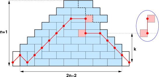
Figure 32. The bijection between modified Aztec $A_{{\mathbf{M}}(k)}$-paths from $(0,0)$ to $(2n,0)$ and the domino tilings of a domain made of the half Aztec diamond (dashed lines), enhanced as indicated, tiled by means of dominos and rigid pairs of $1\times 1$ squares with centers at height $k+2$ and $k$ (depicted in the medallion).

We define modified Aztec paths ($A_{{\mathbf{M}}(k)}$-paths) as the corresponding $\Gamma_{{\mathbf{M}}(k)}$-paths in the ${\mathbb{Z}}_{+}^{2}$ quadrant (without the usual restriction due to $r$ being finite). It has an extra step $(0,-2)$ only from height $h=k+2$ to height $h=k$. The weighting is as in Section 9.2, and the extra step receives a weight $z_{k+2,k}$. Paths from $(0,0)$ to $(2n,0)$ are in bijection with tilings of the domain depicted in Fig.32, by means of the domino tiles of Fig.28, plus rigid pairs of $1\times 1$ defects tiles (see the medallion in Fig.32), with centers at positions $(t-1/2,k)$ and $(t+1/2,k+2)$ with $k+2\leq t\leq 2n-k$, $t$ integer. The “maximal” path $p_{0}$ now involves a succession of $n+1$ up steps $(1,1)$, followed by $n-k$ down steps $(1,-1)$, then one down step $(0,-2)$ and finally $k$ down steps $(1,-1)$. The local moves (i) and (ii) of Fig.30 must now be supplemented by new moves expressing the reduction of the special down steps $(0,-2)$.

The partition function for weighted $A_{{\mathbf{M}}(k)}$-paths is identified with $R_{1,n}$ expressed as a function of ${\mathbf{x}}_{{\mathbf{M}}(k)}$ (up to a multiplicative factor of $R_{1,0}$), choosing the weights $w_{0}=w_{1}=z_{2k+1}=z_{2k+3}=0$, $z_{j}=0$ for $j\geq 2r+4$, $z_{2k+2}=y_{2k+1}$, $z_{j}=y_{j}$ for $j=1,2,...,2k$, and $z_{k+2,k}=y_{k+2,k}=y_{2k}y_{2k+2}/y_{2k+1}$, where the $y_{j}\equiv y_{j}({{\mathbf{M}}(k)})$. Equivalently, $R_{1,n}/R_{1,0}$ is the partition function for weighted tilings of the domain of Figure 32, delimited by the tiles corresponding to the maximal path $p_{0}$, and by the floor at height $h=-1/2$.

For an arbitrary Motzkin path ${\mathbf{M}}$, the $A_{\mathbf{M}}$ Aztec paths are the $\Gamma_{{\mathbf{M}}}$-paths without restriction due to $r$.

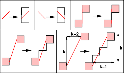
Figure 33. The local rules for constructing the domain ${\mathcal{D}}_{\mathbf{M}}^{(n)}$ out of the maximal $A_{\mathbf{M}}$-path.

Definition 9.5.

The domain ${\mathcal{D}}^{(n)}_{\mathbf{M}}$ is defined as follows. Starting from $\Gamma_{\mathbf{M}}$, remove any down-pointing edges $i\to j$ if $\Gamma_{\mathbf{M}}$ has an edge $i^{\prime}\to j^{\prime}$ with $[j,i]\subset[j^{\prime},i^{\prime}]$ (strict inclusion). This leaves us with a set of “maximal” down-pointing edges. Define the “maximal” path from $(0,0)$ to $(2n,0)$, which has no horizontal step, and goes as far up and to the right as possible, namely starts with a maximal number of steps $(1,1)$, descends via $n$ maximal descending steps. The domain ${\mathcal{D}}^{(n)}_{\mathbf{M}}$ is constructed by associating boundary pieces to each step, as shown in Figure 33. Finally, the domain is completed by a horizontal line at height $h=-1/2$.

Lemma 9.6.

The $A_{\mathbf{M}}$-paths from $(0,0)$ to $(2n,0)$ are in bijection with tilings of the domain ${\mathcal{D}}^{(n)}_{\mathbf{M}}$ by means of the usual $2\times 1$ and $1\times 2$ tiles, plus rigid pairs of square $1\times 1$ tiles centered at points of the form $(t-{i-j-1\over 2},j)$ and $(t+{i-j-1\over 2},i)$ for all the pairs $i,j$ of vertices connected by down-pointing edges on $\Gamma_{\mathbf{M}}$.

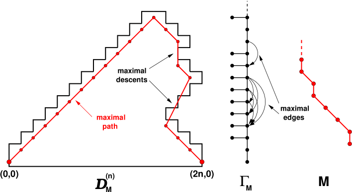
Figure 34. A typical domain ${\mathcal{D}}_{\mathbf{M}}^{(n)}$, with its maximal $A_{\mathbf{M}}$-path (in red), the target graph $\Gamma_{\mathbf{M}}$ and the Motzkin path ${\mathbf{M}}$. We have indicated the two maximal edges, along which the maximal path takes its maximal descents.

We refer to Figure 34 for an example. We can now say that $R_{1,n+m_{1}}/R_{1,m_{1}}$ is the partition function of tilings of ${\mathcal{D}}_{\mathbf{M}}^{(n)}$ as described above.

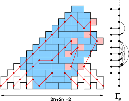
Figure 35. The indented domain ${\mathcal{D}}_{\mathbf{M}}^{(n)}$, serving for the representation of $R_{{\alpha},n}$ in terms of tilings, and the target graph $\Gamma_{\mathbf{M}}$ (here ${\alpha}=3$). Note that the tiling involves defect pairs corresponding to descents of $\Gamma_{\mathbf{M}}$, and that horizontal edges (tiles $d$) are forbidden at heights where $\Gamma_{\mathbf{M}}$ has no horizontal edges. Outside of the shaded blue domain, all the tiles are fixed by the indentations and the absence of $d$ tile in the bottom row.

Finally, recall that $R_{{\alpha},n+m_{1}}/(R_{1,m_{1}})^{n}$ is the generating function for families of ${\alpha}$ strongly non-intersecting $\Gamma_{\mathbf{M}}$-paths, starting at $(0,0),...,(2{\alpha}-2,0)$ and ending at $(2n,0),...,(2n+2{\alpha}-2,0)$. These paths can be represented as tilings of the domain ${\mathcal{D}}_{\mathbf{M}}^{(n)}$ with ${\alpha}-1$ additional indentations on the bottom left and bottom right boundary (see Fig.35), by means of dominos and rigid defect pairs corresponding to down-pointing edges of $\Gamma_{\mathbf{M}}$. The strong non-intersection of the paths imposes extra constraints on the tilings, by forbiding some local configurations.

10. Conclusion

In this paper, we found a simple structural explanation for the cluster mutations, which allow for sweeping the set of possible initial data for the $Q$-system, in terms of simple local rearrangements of the continued fractions that generate the $R_{1,n}$’s. This local move allowing for generating mutations is reminiscent of the local “Yang-Baxter”-like relation used in [8] in the context of total positivity of the Grassmannian, as expressed through local positive transfer matrices for networks. We do not yet fully undertand this relation, although a partial explanation is found in [5].

In view of Example 6.8, we can think of the constructions of this paper as generalizations of the Stieltjes theorem [23], that now allow to re-express the series $F(\lambda)=\sum_{k\geq 0}(-1)^{k}a_{k}/\lambda^{k+1}$ in different ways as (mutated) possibly multiply branching continued fractions, whose coefficients are particular combinations of Hankel determinants involving the sequence $a_{k}$, each such rewriting corresponding to a Motzkin path. To make the contact with our results, we simply have to take $t=-1/\lambda$, $a_{k}=R_{1,k}$ and to identify $R_{{\alpha},n}=\Delta_{\alpha}^{n-{\alpha}+1}$ with the Hankel determinants of eq.(6.27). For each Motzkin path ${\mathbf{M}}$, we find a new continued fraction expression for $F(\lambda)$ involving only the Hankel determinants corresponding to the cluster variable ${\mathbf{x}}_{\mathbf{M}}$, via the weights $y_{i}({\mathbf{M}})$.

Equations called $Q$-systems exist for all simple Lie algebras. We have checked that in these cases, $R_{1,n}$ also satisfies linear recursion relations with constant coefficients. We expect the constructions of the present paper to generalize to all these cases. In particular, we expect cluster positivity to be a consequence of the LGV formula applied to counting possibly interacting families of non-intersecting paths.

The $Q$-system is a specialization of the $T$-sytem, a discrete integrable system with one additional parameter. It was shown in [4] that $T$-systems can be considered as cluster algebras, in general, of infinite rank. The statistical models in this paper are particularly well-suited to the solution of the $T$-system [6].

In the case of the cluster variables corresponding to seeds of the cluster algebra outside the subgraph $\mathcal{G}_{r}$, we do not have an interpretation in terms of a statistical model. Outside this subgraph, the exchange matrix $B$ has entries which grow arbitrarily. This seems to suggest that the evolution in directions leading outside $\mathcal{G}_{r}$ is not integrable.

Appendix A The case of $A_{3}$ in the heap formulation.

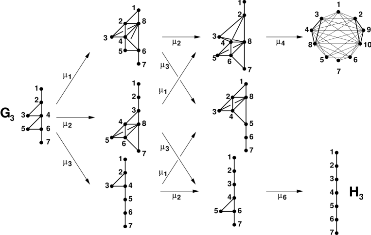
Figure 36. The heap graphs corresponding to the $R_{1,n}$’s for the case $A_{3}$, and the corresponding mutations of seeds.

In this appendix, we detail the heap interpretation of the solution $R_{1,n}$ of the $A_{3}$ $Q$-system, as expressed in terms of the various cluster variables corresponding to the 9 seeds of the fundamental domain. We apply the same systematic method as in Example 4.8. For simplicity, we have just depicted in Fig.36 the heap graphs, together with the mutations relating them, for each cluster variable of the fundamental domain. The corresponding rearrangements of the generating function $F_{1}^{(3)}(t)$ and new weights are given below, with the labeling of vertices indicated in Fig.36. These are straightforwardly generated by carefully following the successive applications of Lemmas 4.5 and 4.6.

Initial cluster variable: $G_{3}$. We start from the graph $G_{3}$ and the associated heap generating function $F_{1}^{(3)}(t)=1+ty_{1}\Phi^{(G_{3})}(t)$, with

$$\Phi^{(G_{3})}(t)={1\over 1-ty_{1}-t{y_{2}\over 1-ty_{3}-t{y_{4}\over 1-ty_{5}-t{y_{6}\over 1-ty_{7}}}}}$$

with the $y$’s as in (3.17), namely

$$y_{1}={R_{1,1}\over R_{1,0}},y_{2}={R_{2,1}\over R_{1,0}R_{1,1}},y_{3}={R_{1,0}R_{2,1}\over R_{2,0}R_{1,1}},y_{4}={R_{1,0}R_{3,1}\over R_{2,0}R_{2,1}},y_{5}={R_{2,0}R_{3,1}\over R_{3,0}R_{2,1}},y_{6}={R_{2,0}\over R_{3,0}R_{3,1}},y_{7}={R_{3,0}\over R_{3,1}}.$$

Note that the weights are related via $y_{1}y_{3}y_{5}y_{7}=1$.

Mutation $\mu_{1}(G_{3})$. We apply Lemma 4.6 to vertices $1$, $2$ and the structure attached to $3$. This gives $F_{1}^{(3)}(t)=1+ty_{1}\Phi^{(\mu_{1}(G_{3}))}(t)$, with

$$\Phi^{(\mu_{1}(G_{3}))}(t)={1\over 1-t{z_{1}\over 1-t{z_{2}+{z_{8}\over 1-tz_{5}-t{z_{6}\over 1-tz_{7}}}\over 1-tz_{3}-t{z_{4}\over 1-tz_{5}-t{z_{6}\over 1-tz_{7}}}}}}$$

with

$$z_{1}=y_{1}+y_{2},z_{2}={y_{2}y_{3}\over y_{1}+y_{2}},z_{8}={y_{2}y_{4}\over y_{1}+y_{2}},z_{3}={y_{1}y_{3}\over y_{1}+y_{2}},z_{4}={y_{1}y_{4}\over y_{1}+y_{2}},z_{5}=y_{5},z_{6}=y_{6},z_{7}=y_{7}$$

namely, upon using the $Q$-system relation $R_{1,0}R_{1,2}=R_{1,1}^{2}+R_{2,1}$:

$$z_{1}={R_{1,2}\over R_{1,1}},z_{2}={R_{2,1}^{2}\over R_{2,0}R_{1,1}R_{1,2}},z_{3}={R_{1,1}R_{2,1}\over R_{2,0}R_{1,2}},z_{4}={R_{1,1}^{2}R_{3,1}\over R_{2,0}R_{2,1}R_{1,2}},$$

$$z_{5}={R_{2,0}R_{3,1}\over R_{3,0}R_{2,1}},z_{6}={R_{2,0}\over R_{3,0}R_{3,1}},z_{7}={R_{3,0}\over R_{3,1}},z_{8}={R_{3,1}\over R_{2,0}R_{1,2}}.$$

Note that there is one more $z$ than $y$’s, but that we now have two relations $z_{1}z_{3}z_{5}z_{7}=1$ and $z_{3}z_{8}=z_{2}z_{4}$.

Mutation $\mu_{2}(G_{3})$. We apply Lemma 4.6 to vertices $3$, $4$ and the descendent structure attached to $4$. This gives $F_{1}^{(3)}(t)=1+ty_{1}\Phi^{(\mu_{2}(G_{3}))}(t)$, with

$$\Phi^{(\mu_{2}(G_{3}))}(t)={1\over 1-tx_{1}-t{x_{2}\over 1-t{x_{3}\over 1-t{x_{4}+{x_{8}\over 1-tx_{7}}\over 1-tx_{5}-t{x_{6}\over 1-tx_{7}}}}}}$$

with

$$x_{1}=y_{1},x_{2}=y_{2},x_{3}=y_{3}+y_{4},x_{4}={y_{4}y_{5}\over y_{3}+y_{4}},x_{8}={y_{4}y_{6}\over y_{3}+y_{4}},x_{5}={y_{3}y_{5}\over y_{3}+y_{4}},x_{6}={y_{3}y_{6}\over y_{3}+y_{4}},x_{7}=y_{7}.$$

namely, upon using the $Q$-system relation $R_{2,0}R_{2,2}=R_{2,1}^{2}+R_{1,1}R_{3,1}$:

$$x_{1}={R_{1,1}\over R_{1,0}},x_{2}={R_{2,1}\over R_{1,0}R_{1,1}},x_{3}={R_{1,0}R_{2,2}\over R_{1,1}R_{2,1}},x_{4}={R_{1,1}R_{3,1}^{2}\over R_{3,0}R_{2,1}R_{2,2}},$$

$$x_{5}={R_{2,1}R_{3,1}\over R_{3,0}R_{2,2}},x_{6}={R_{2,1}^{2}\over R_{3,0}R_{3,1}R_{2,2}},x_{7}={R_{3,0}\over R_{3,1}},x_{8}={R_{1,1}\over R_{3,0}R_{2,2}}.$$

As for the $z$’s above, there is one more $x$ than $y$’s, but they obey two relations: $x_{1}x_{3}x_{5}x_{7}=1$ and $x_{5}x_{8}=x_{4}x_{6}$.

Mutation $\mu_{3}(G_{3})$. This is part of the sequence of graphs of Example 5.6. It is obtained by applying the Lemma 4.6 to the vertices $5,6,7$ of $G_{3}$. This gives $F_{1}^{(3)}(t)=1+ty_{1}\Phi^{(\mu_{3}(G_{3}))}(t)$, with

$$\Phi^{(\mu_{3}G_{3})}(t)={1\over 1-t\,t_{1}-t{t_{2}\over 1-t\,t_{3}-t{t_{4}\over 1-t{t_{5}\over 1-t{t_{6}\over 1-t\,t_{7}}}}}}$$

with

$$t_{1}=y_{1},t_{2}=y_{2},t_{3}=y_{3},t_{4}=y_{4},t_{5}=y_{5}+y_{6},t_{6}={y_{6}y_{7}\over y_{5}+y_{6}},t_{7}={y_{5}y_{7}\over y_{5}+y_{6}}.$$

namely, upon using the $Q$-system relation $R_{3,0}R_{3,2}=R_{3,1}^{2}+R_{2,1}$:

$$t_{1}={R_{1,1}\over R_{1,0}},t_{2}={R_{2,1}\over R_{1,0}R_{1,1}},t_{3}={R_{1,0}R_{2,1}\over R_{2,0}R_{1,1}},t_{4}={R_{1,0}R_{3,1}\over R_{2,0}R_{2,1}},t_{5}={R_{2,0}R_{3,2}\over R_{2,1}R_{3,1}},t_{6}={R_{2,1}\over R_{3,1}R_{3,2}},t_{7}={R_{3,1}\over R_{3,2}}.$$

Note that the $t$ satisfy the relation $t_{1}t_{3}t_{5}t_{7}=1$.

Mutation $\mu_{1}\mu_{2}(G_{3})$. We apply Lemma 4.6 to the vertices $1$, $2$, and the substructure attached to $3$ in the graph $\mu_{2}(G_{3})$ (see Fig.36). This gives $\Phi^{(\mu_{1}\mu_{2}(G_{3}))}(t)=\Phi^{(\mu_{2}(G_{3}))}(t)$, with

(A.1) $$\Phi^{(\mu_{1}\mu_{2}(G_{3}))}(t)={1\over 1-t{u_{1}\over 1-t{u_{2}\over 1-tu_{3}-t{u_{4}+{u_{8}\over 1-tu_{7}}\over 1-tu_{5}-t{u_{6}\over 1-tu_{7}}}}}}$$

with

$$u_{1}=x_{1}+x_{2},u_{2}={x_{2}x_{3}\over x_{1}+x_{2}},u_{3}={x_{1}x_{3}\over x_{1}+x_{2}},u_{4}=x_{4},u_{5}=x_{5},u_{6}=x_{6},u_{7}=x_{7},u_{8}=x_{8}.$$

namely, upon using the $Q$-system relation $R_{1,0}R_{1,2}=R_{1,1}^{2}+R_{2,1}$:

$$u_{1}={R_{1,2}\over R_{1,1}},u_{2}={R_{2,2}\over R_{1,1}R_{1,2}},u_{3}={R_{1,1}R_{2,2}\over R_{1,2}R_{2,1}},u_{4}={R_{1,1}R_{3,1}^{2}\over R_{3,0}R_{2,1}R_{2,2}}$$

$$u_{5}={R_{2,1}R_{3,1}\over R_{3,0}R_{2,2}},u_{6}={R_{2,1}^{2}\over R_{3,0}R_{3,1}R_{2,2}},u_{7}={R_{3,0}\over R_{3,1}},u_{8}={R_{1,1}\over R_{3,0}R_{2,2}}.$$

Note that the $u$’s satisfy the two relations $u_{1}u_{3}u_{5}u_{7}=1$ and $u_{5}u_{8}=u_{4}u_{6}$. It is instructive to see how to arrive at the same result from the sequence of mutations $\mu_{2}\mu_{1}(G_{3})=\mu_{1}\mu_{2}(G_{3})$. We now start from the graph $\mu_{1}(G_{3})$, and apply the Lemma 4.6 with (i) the vertex 2 and its substructure, (ii) the vertex 8 and its substructure common with that of vertex 2 (iii) its attached substructure not common with that of the vertex 2, namely with

$$a = {z_{2}\over 1-tz_{3}-t{z_{4}\over 1-tz_{5}-t{z_{6}\over 1-tz_{7}}}}$$

$$b = {z_{8}\over 1-tz_{3}-t{z_{4}\over 1-tz_{5}-t{z_{6}\over 1-tz_{7}}}}$$

$$c = z_{5}+{z_{6}\over 1-tz_{7}}$$

The result is

(A.2) $$\Phi^{(\mu_{2}\mu_{1}(G_{3}))}(t)={1\over 1-t{u_{1}^{\prime}\over 1-t{u_{2}^{\prime}\over\left(1-tz_{3}-t{z_{4}\over 1-tz_{5}-t{z_{6}\over 1-tz_{7}}}\right)\left(1-t{u_{4}^{\prime}+{u_{8}^{\prime}\over 1-tu_{7}^{\prime}}\over 1-tu_{5}^{\prime}-t{u_{6}^{\prime}\over 1-tu_{7}^{\prime}}}\right)}}}$$

with

$$u_{1}^{\prime}=z_{1}=y_{1}+y_{2}=u_{1},u_{2}^{\prime}=z_{2}+z_{8}=y_{2}{y_{3}+y_{4}\over y_{1}+y_{2}}={x_{2}x_{3}\over x_{1}+x_{2}}=u_{2},$$

$$u_{4}^{\prime}={z_{8}z_{5}\over z_{2}+z_{8}}={y_{4}y_{5}\over y_{3}+y_{4}}=x_{4}=u_{4},u_{8}^{\prime}={z_{8}z_{6}\over z_{2}+z_{8}}={y_{4}y_{6}\over y_{3}+y_{4}}=x_{8}=u_{8},$$

$$u_{5}^{\prime}={z_{2}z_{5}\over z_{2}+z_{8}}=x_{5}=u_{5},u_{6}^{\prime}={z_{2}z_{6}\over z_{2}+z_{8}}={y_{3}y_{6}\over y_{3}+y_{4}}=x_{6}=u_{6},u_{7}^{\prime}=z_{7}=x_{7}=u_{7},$$

where we have used the expressions of the $z$’s and the $x$’s in terms of the $y$’s. Applying again Lemma 4.6 to the first factor under $u_{2}^{\prime}$, with $a=z_{3}$, $b=z_{4}$, $c=z_{5}+z_{6}/(1-tz_{7})$, we may rewrite:

(A.3) $$z_{3}+{z_{4}\over 1-tz_{5}-t{z_{6}\over 1-tz_{7}}}={u_{3}^{\prime}\over 1-t{u_{4}^{\prime\prime}\over 1-tu_{5}^{\prime\prime}-t{u_{6}^{\prime\prime}\over 1-tu_{7}^{\prime\prime}}}}$$

with

$$u_{3}^{\prime}=z_{3}+z_{4}=y_{1}{y_{3}+y_{4}\over y_{1}+y_{2}}={x_{1}x_{3}\over x_{1}+x_{2}}=u_{3},u_{4}^{\prime\prime}={z_{4}z_{5}\over z_{3}+z_{4}}={z_{8}z_{5}\over z_{2}+z_{8}}=u_{4}^{\prime}=u_{4},$$

$$u_{5}^{\prime\prime}={z_{3}z_{5}\over z_{3}+z_{4}}={z_{2}z_{5}\over z_{2}+z_{8}}=u_{5}^{\prime}=u_{5},u_{7}^{\prime\prime}=z_{7}=u_{7},$$

where we have used the relation $z_{3}/z_{4}=z_{2}/z_{8}$ between the $z$’s. Substituting this into (A.2), we finally recover eq.(A.1). This case is made particularly cumbersome by the fact that the vertex 2 contains a substructure (which has not yet been the case so far), encoded in the fraction (A.3). From this example, we learn that the mutation $\mu_{2}$ consists actually of two simultaneous applications of the Lemma 4.6, one “usual” and one within the substructure attached to the initial vertex 2.

Mutation $\mu_{1}\mu_{3}(G_{3})$. We apply Lemma 4.6 to the vertices $1$, $2$, and the substructure attached to $2$ in the graph $\mu_{3}(G_{3})$ (see Fig.36). This gives $\Phi^{(\mu_{1}\mu_{3}(G_{3}))}(t)=\Phi^{(\mu_{3}(G_{3}))}(t)$, with

(A.4) $$\Phi^{(\mu_{1}\mu_{3}(G_{3}))}(t)={1\over 1-t{w_{1}\over 1-t\left({w_{2}+{w_{8}\over 1-t{w_{5}\over 1-t{w_{6}\over 1-tw_{7}}}}\over 1-tw_{3}-t{w_{4}\over 1-t{w_{5}\over 1-t{w_{6}\over 1-tw_{7}}}}}\right)}}$$

with

$$w_{1}=t_{1}+t_{2},w_{2}={t_{2}t_{3}\over t_{1}+t_{2}},w_{8}={t_{2}t_{4}\over t_{1}+t_{2}},w_{3}={t_{1}t_{3}\over t_{1}+t_{2}},w_{4}={t_{1}t_{4}\over t_{1}+t_{2}},w_{5}=t_{5},w_{6}=t_{6},w_{7}=t_{7}.$$

namely, upon using the $Q$-system relation $R_{1,0}R_{1,2}=R_{1,1}^{2}+R_{2,1}$:

$$w_{1}={R_{1,2}\over R_{1,1}},w_{2}={R_{2,1}^{2}\over R_{2,0}R_{1,1}R_{1,2}},w_{3}={R_{3,1}\over R_{1,2}R_{2,0}},w_{4}={R_{1,1}^{2}R_{3,1}\over R_{2,0}R_{2,1}R_{1,2}},$$

$$w_{5}={R_{2,0}R_{3,2}\over R_{2,1}R_{3,1}},w_{6}={R_{2,1}\over R_{3,1}R_{3,2}},w_{7}={R_{3,1}\over R_{3,2}},w_{8}={R_{3,1}\over R_{2,0}R_{1,2}}.$$

Note the relations: $w_{1}w_{3}w_{5}w_{7}=1$ and $w_{2}w_{4}=w_{3}w_{8}$. For completeness, let us compute the function $\Phi^{(\mu_{3}\mu_{1}(G_{3}))}=\Phi^{(\mu_{1}(G_{3}))}$, and check that indeed $\mu_{1}\mu_{3}(G_{3})=\mu_{3}\mu_{1}(G_{3})$ yield the same result. We now apply the Lemma 4.6 with the vertices 5, 6 and 7 of the graph $\mu_{1}(G_{3})$, with respectively $a=z_{5}$, $b=z_{6}$ and $c=z_{7}$, while $d=0$. This gives

(A.5) $$\Phi^{(\mu_{3}\mu_{1}(G_{3}))}={1\over 1-t{w_{1}^{\prime}\over 1-t{w_{2}^{\prime}+{w_{8}^{\prime}\over 1-t{w_{5}^{\prime}\over 1-t{w_{6}^{\prime}\over 1-tw_{7}^{\prime}}}}\over 1-tw_{3}^{\prime}-t{w_{4}^{\prime}\over 1-t{w_{5}^{\prime}\over 1-t{w_{6}^{\prime}\over 1-tw_{7}^{\prime}}}}}}}$$

with

$$w_{1}^{\prime}=z_{1}=y_{1}+y_{2}=t_{1}+t_{2}=w_{1},\ \ w_{2}^{\prime}=z_{2}={y_{2}y_{3}\over y_{1}+y_{2}}={t_{2}t_{3}\over t_{1}+t_{2}}=w_{2}$$

$$w_{8}^{\prime}=z_{8}={y_{2}y_{4}\over y_{1}+y_{2}}={t_{2}t_{4}\over t_{1}+t_{2}}=w_{8},\ \ w_{3}^{\prime}=z_{3}={y_{1}y_{3}\over y_{1}+y_{2}}={t_{1}t_{3}\over t_{1}+t_{2}}=w_{3},$$

$$w_{4}^{\prime}=z_{4}={y_{1}y_{4}\over y_{1}+y_{2}}={t_{1}t_{4}\over t_{1}+t_{2}}=w_{4},\ \ w_{5}^{\prime}=z_{5}+z_{6}=y_{5}+y_{6}=t_{5}=w_{5},$$

$$w_{6}^{\prime}={z_{6}z_{7}\over z_{5}+z_{6}}={y_{6}y_{7}\over y_{5}+y_{6}}=t_{6}=w_{6},\ \ w_{7}^{\prime}={z_{5}z_{7}\over z_{5}+z_{6}}={y_{5}y_{7}\over y_{5}+y_{6}}=t_{7}=w_{7},$$

where the various identifications are made by use of the expressions of the $z$’s and $t$’s in terms of the $y$’s. We deduce that the expressions (A.4) and (A.5) are identical.

Mutation $\mu_{2}\mu_{3}(G_{3})$. This is part of the sequence of graphs of Example 5.6. It is obtained by applying the Lemma 4.6 to the vertices $3,4$ and the structure attached to $5$ of the graph $\mu_{3}(G_{3})$ (see Fig.36). This gives $\Phi^{(\mu_{2}\mu_{3}(G_{3}))}(t)=\Phi^{(\mu_{3}(G_{3}))}(t)$, with

(A.6) $$\Phi^{(\mu_{2}\mu_{3}(G_{3}))}(t)={1\over 1-ts_{1}-t{s_{2}\over 1-t{s_{3}\over 1-t{s_{4}\over 1-ts_{5}-t{s_{6}\over 1-ts_{7}}}}}}$$

with

$$s_{1}=t_{1},s_{2}=t_{2},s_{3}=t_{3}+t_{4},s_{4}={t_{4}t_{5}\over t_{3}+t_{4}},s_{5}={t_{3}t_{5}\over t_{3}+t_{4}},s_{6}=t_{6},s_{7}=t_{7}.$$

namely, upon using the $Q$-system relation $R_{2,0}R_{2,2}=R_{2,1}^{2}+R_{1,1}R_{3,1}$:

$$s_{1}={R_{1,1}\over R_{1,0}},s_{2}={R_{2,1}\over R_{1,0}R_{1,1}},s_{3}={R_{1,0}R_{2,2}\over R_{1,1}R_{2,1}},s_{4}={R_{1,1}R_{3,2}\over R_{2,1}R_{2,2}},s_{5}={R_{2,1}R_{3,2}\over R_{3,1}R_{2,2}},s_{6}={R_{2,1}\over R_{3,1}R_{3,2}},s_{7}={R_{3,1}\over R_{3,2}}.$$

Note the relation $s_{1}s_{3}s_{5}s_{7}=1$. For completeness, let us compute the function $\Phi^{(\mu_{3}\mu_{2}(G_{3}))}=\Phi^{(\mu_{2}(G_{3}))}$, and check that indeed $\mu_{2}\mu_{3}(G_{3})=\mu_{3}\mu_{2}(G_{3})$ yield the same result. We now apply the Lemma 4.6 on the graph $\mu_{2}(G_{3})$, with (i) the vertex 4 and its substructure (ii) the vertex 8 and its substructure common to vertex 4, and the substructure of vertex $8$ not common to vertex 4. This amounts to taking $a=x_{4}/(1-tx_{5}-tx_{6}/(1-tx_{7}))$, $b=x_{8}/(1-tx_{5}-tx_{6}/(1-tx_{7}))$ and $c=x_{7}$, while $d=0$. This yields

(A.7) $$\Phi^{(\mu_{3}\mu_{2}(G_{3}))}={1\over 1-ts_{1}^{\prime}-t{s_{2}^{\prime}\over 1-t{s_{3}^{\prime}\over 1-t{s_{4}^{\prime}\over\left(1-tx_{5}-t{x_{6}\over 1-tx_{7}}\right)\left(1-t{s_{6}^{\prime}\over 1-ts_{7}^{\prime}}\right)}}}}$$

with

$$s_{1}^{\prime}=x_{1}=y_{1}=t_{1}=s_{1},\ s_{2}^{\prime}=x_{2}=y_{2}=t_{2}=s_{2},\ s_{3}^{\prime}=x_{3}=y_{3}+y_{4}=t_{3}+t_{4}=s_{3},$$

$$s_{4}^{\prime}=x_{4}+x_{8}=y_{4}{y_{5}+y_{6}\over y_{3}+y_{4}}={t_{4}t_{5}\over t_{3}+t_{4}}=s_{4},\ s_{6}^{\prime}={x_{7}x_{8}\over x_{4}+x_{8}}={y_{6}y_{7}\over y_{5}+y_{6}}=t_{6}=s_{6},$$

$$s_{7}^{\prime}={x_{7}x_{4}\over x_{4}+x_{8}}={y_{5}y_{7}\over y_{5}+y_{6}}=t_{7}=s_{7},$$

where identifications are made by expressing the $x$’s, $s$’s and $t$’s in terms of the $y$’s. As in the case of $\mu_{2}\mu_{1}(G_{3})$, we see that we must still apply the Lemma 4.6 to the first factor under $s_{4}^{\prime}$ in (A.7), which corresponds to the substructure attached to the initial vertex 4. This allows to rewrite

$$x_{5}+{x_{6}\over 1-tx_{7}}={s_{5}^{\prime\prime}\over 1-t{s_{6}^{\prime\prime}\over 1-ts_{7}^{\prime\prime}}}$$

with

$$s_{5}^{\prime\prime}=x_{5}+x_{6}=y_{3}{y_{5}+y_{6}\over y_{3}+y_{4}}={t_{3}t_{5}\over t_{3}+t_{4}}=s_{5},\ \ s_{6}^{\prime\prime}={x_{6}x_{7}\over x_{5}+x_{6}}={y_{6}y_{7}\over y_{5}+y_{6}}=t_{6}=s_{6}$$

$$s_{7}^{\prime\prime}={x_{5}x_{7}\over x_{5}+x_{6}}={y_{5}y_{7}\over y_{5}+y_{6}}=t_{7}=s_{7}.$$

Substituting these into (A.7) allows to identify it with (A.6).

Mutation $\mu_{6}\mu_{2}\mu_{3}(G_{3})=H_{3}$. This is part of the sequence of graphs of Example 5.6. It is obtained by applying the Lemma 4.6 to the vertices $5,6,7$ of the graph $\mu_{2}\mu_{3}(G_{3})$ (see Fig.36). This gives $\Phi^{(\mu_{6}\mu_{2}\mu_{3}(G_{3}))}(t)=\Phi^{(\mu_{2}\mu_{3}(G_{3}))}(t)$, with

$$\Phi^{(\mu_{6}\mu_{2}\mu_{3}(G_{3}))}(t)={1\over 1-tr_{1}-t{r_{2}\over 1-t{r_{3}\over 1-t{r_{4}\over 1-t{r_{5}\over 1-t{r_{6}\over 1-tr_{7}}}}}}}$$

with

$$r_{1}=s_{1},r_{2}=s_{2},r_{3}=s_{3},r_{4}=s_{4},r_{5}=s_{5}+s_{6},r_{6}={s_{6}s_{7}\over s_{5}+s_{6}},r_{7}={s_{5}s_{7}\over s_{5}+s_{6}}.$$

namely, upon using the $Q$-system relation $R_{3,1}R_{3,3}=R_{3,2}^{2}+R_{2,2}$:

$$r_{1}={R_{1,1}\over R_{1,0}},r_{2}={R_{2,1}\over R_{1,0}R_{1,1}},r_{3}={R_{1,0}R_{2,2}\over R_{1,1}R_{2,1}},r_{4}={R_{1,1}R_{3,2}\over R_{2,1}R_{2,2}},r_{5}={R_{2,1}R_{3,3}\over R_{2,2}R_{3,2}},r_{6}={R_{2,2}\over R_{3,2}R_{3,3}},r_{7}={R_{3,2}\over R_{3,3}}.$$

Note the relation $r_{1}r_{3}r_{5}r_{7}=1$.

Mutation $\mu_{4}\mu_{1}\mu_{2}(G_{3})$. It is obtained by applying the Lemma 4.6 to the vertices $1,2$ and the structure attached to $2$ of the graph $\mu_{1}\mu_{2}(G_{3})$ (see Fig.36). Writing $\Phi^{(\mu_{1}\mu_{2}(G_{3}))}(t)=1+tu_{1}\Psi^{(\mu_{1}\mu_{2}(G_{3}))}(t)$, we have $\Psi^{(\mu_{4}\mu_{1}\mu_{2}(G_{3}))}(t)=\Psi^{(\mu_{1}\mu_{2}(G_{3}))}(t)$, with

(A.8) $$\Psi^{(\mu_{4}\mu_{1}\mu_{2}(G_{3}))}(t)={1\over 1-t{v_{1}\over 1-t\left({v_{2}+{v_{9}+{v_{10}\over 1-tv_{7}}\over 1-tv_{5}-t{v_{6}\over 1-tv_{7}}}\over 1-t\left(v_{3}+{v_{4}+{v_{8}\over 1-tv_{7}}\over 1-tv_{5}-t{v_{6}\over 1-tv_{7}}}\right)}\right)}}$$

with

$$v_{1}=u_{1}+u_{2},v_{2}={u_{2}u_{3}\over u_{1}+u_{2}},v_{9}={u_{2}u_{4}\over u_{1}+u_{2}},v_{10}={u_{2}u_{8}\over u_{1}+u_{2}},v_{3}={u_{1}u_{3}\over u_{1}+u_{2}},$$

$$v_{4}={u_{1}u_{4}\over u_{1}+u_{2}},v_{5}=u_{5},v_{6}=u_{6},v_{7}=u_{7},v_{8}={u_{1}u_{8}\over u_{1}+u_{2}}.$$

namely, upon using the $Q$-system relation $R_{1,1}R_{1,3}=R_{1,2}^{2}+R_{2,2}$:

$$v_{1}={R_{1,3}\over R_{1,2}},v_{2}={R_{2,2}^{2}\over R_{2,1}R_{1,2}R_{1,3}},v_{3}={R_{1,2}R_{2,2}\over R_{2,1}R_{1,3}},v_{4}={R_{1,2}^{2}R_{3,1}^{2}\over R_{3,0}R_{2,1}R_{2,2}R_{1,3}},v_{5}={R_{2,1}R_{3,1}\over R_{3,0}R_{2,2}}$$

$$v_{6}={R_{2,1}^{2}\over R_{3,0}R_{3,1}R_{2,2}},v_{7}={R_{3,0}\over R_{3,1}},v_{8}={R_{1,2}^{2}\over R_{3,0}R_{2,2}R_{1,3}},v_{9}={R_{3,1}^{2}\over R_{3,0}R_{2,1}R_{1,3}},v_{10}={1\over R_{3,0}R_{1,3}}.$$

Note that as we have 3 more $v$’s than $y$’s, we expect four relations between them. These read: $v_{1}v_{3}v_{5}v_{7}=1$, $v_{2}v_{4}=v_{3}v_{9}$, $v_{8}v_{9}=v_{4}v_{10}$ and $v_{2}v_{8}=v_{3}v_{10}$.

We conclude that for $r=3$, $R_{1,n}$ is a positive Laurent polynomial of all the mutations of the initial data ${\mathbf{x}}_{0}$ in the fundamental domain ${\mathcal{F}}_{3}$.

Appendix B The case of $A_{3}$ in the path formulation.

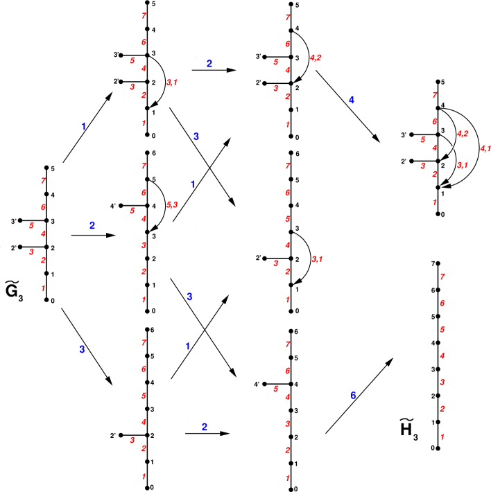
Figure 37. The target graphs $\Gamma_{\mathbf{M}}$ for the nine seeds of the case $A_{3}$ (labelled by the 9 Motzkin paths of Fig.2), and the corresponding mutations. We have indicated vertex and edge labels.

In this appendix, we detail the path interpretation of the solution $R_{1,n}$ of the $A_{3}$ $Q$-system, as expressed in terms of the various initial data corresponding to the 9 cluster variables of the fundamental domain ${\mathcal{F}}_{3}$, labelled by the 9 Motzkin paths of Fig.2.

As a direct illustration of the constructions of Section 6, we list below for each of the nine cluster variables the corresponding transfer matrix $T_{\Gamma}$, and the generating function $\left((I-T_{\Gamma})^{-1}\right)_{0,0}$, in terms of dummy weights $y_{i}$ and $y_{i,j}$, that are actually shorthand notations for the weights $y_{i}({\mathbf{M}})$ and their redundant counterparts, to be extracted from Theorem 6.7 and eq.(5.5). The corresponding graphs are represented in Fig.37, together with the mutations relating the associated cluster variables.

For ${\mathbf{M}}_{0}=\bf\{(0,1),(0,2),(0,3)\}$: The corresponding target graph is $\Gamma_{{\mathbf{M}}_{0}}={\tilde{G}}_{3}$. The transfer matrix and the associated generating function are:

$$T_{\Gamma_{{\mathbf{M}}_{0}}}={\small\left(\begin{matrix}0&ty_{1}&0&0&0&0&0&0\\ 1&0&ty_{2}&0&0&0&0&0\\ 0&1&0&ty_{3}&ty_{4}&0&0&0\\ 0&0&1&0&0&0&0&0\\ 0&0&1&0&0&ty_{5}&ty_{6}&0\\ 0&0&0&0&1&0&0&0\\ 0&0&0&0&1&0&0&ty_{7}\\ 0&0&0&0&0&0&1&0\end{matrix}\right)},\quad\left((I-T_{\Gamma_{{\mathbf{M}}_{0}}})^{-1}\right)_{0,0}={1\over 1-t{y_{1}\over 1-t{y_{2}\over 1-ty_{3}-t{y_{4}\over 1-ty_{5}-t{y_{6}\over 1-ty_{7}}}}}}$$

For ${\mathbf{M}}_{1}=\bf\mu_{1}{\mathbf{M}}_{0}=\{(1,1),(0,2),(0,3)\}$, with $y_{3,1}=y_{2}y_{4}/y_{3}$:

$$T_{\Gamma_{{\mathbf{M}}_{1}}}={\small\left(\begin{matrix}0&ty_{1}&0&0&0&0&0&0\\ 1&0&ty_{2}&0&ty_{3,1}&0&0&0\\ 0&1&0&ty_{3}&ty_{4}&0&0&0\\ 0&0&1&0&0&0&0&0\\ 0&0&1&0&0&ty_{5}&ty_{6}&0\\ 0&0&0&0&1&0&0&0\\ 0&0&0&0&1&0&0&ty_{7}\\ 0&0&0&0&0&0&1&0\end{matrix}\right)},\quad\left((I-T_{\Gamma_{{\mathbf{M}}_{1}}})^{-1}\right)_{0,0}={1\over 1-t{y_{1}\over 1-t{y_{2}+{y_{3,1}\over 1-ty_{5}-t{y_{6}\over 1-ty_{7}}}\over 1-ty_{3}-t{y_{4}\over 1-ty_{5}-t{y_{6}\over 1-ty_{7}}}}}}.$$

For ${\mathbf{M}}_{2}=\bf\mu_{2}{\mathbf{M}}_{0}=\{(0,1),(1,2),(0,3)\}$, with $y_{5,3}=y_{4}y_{6}/y_{5}$:

$$T_{\Gamma_{{\mathbf{M}}_{2}}}={\small\left(\begin{matrix}0&ty_{1}&0&0&0&0&0&0\\ 1&0&ty_{2}&0&0&0&0&0\\ 0&1&0&ty_{3}&0&0&0&0\\ 0&0&1&0&ty_{4}&0&ty_{5,3}&0\\ 0&0&0&1&0&ty_{5}&ty_{6}&0\\ 0&0&0&0&1&0&0&0\\ 0&0&0&0&1&0&0&ty_{7}\\ 0&0&0&0&0&0&1&0\end{matrix}\right)}\quad\left((I-T_{\Gamma_{{\mathbf{M}}_{2}}})^{-1}\right)_{0,0}={1\over 1-t{y_{1}\over 1-t{y_{2}\over 1-t{y_{3}\over 1-t{y_{4}+{y_{5,3}\over 1-ty_{7}}\over 1-ty_{5}-t{y_{6}\over 1-ty_{7}}}}}}}.$$

For ${\mathbf{M}}_{3}=\bf\mu_{3}{\mathbf{M}}_{0}=\{(0,1),(0,2),(1,3)\}$:

$$T_{\Gamma_{{\mathbf{M}}_{3}}}={\small\left(\begin{matrix}0&ty_{1}&0&0&0&0&0&0\\ 1&0&ty_{2}&0&0&0&0&0\\ 0&1&0&ty_{3}&ty_{4}&0&0&0\\ 0&0&1&0&0&0&0&0\\ 0&0&1&0&0&ty_{5}&0&0\\ 0&0&0&0&1&0&ty_{6}&0\\ 0&0&0&0&0&1&0&ty_{7}\\ 0&0&0&0&0&0&1&0\end{matrix}\right)},\quad\left((I-T_{\Gamma_{{\mathbf{M}}_{3}}})^{-1}\right)_{0,0}={1\over 1-t{y_{1}\over 1-t{y_{2}\over 1-ty_{3}-t{y_{4}\over 1-t{y_{5}\over 1-t{y_{6}\over 1-ty_{7}}}}}}}.$$

For ${\mathbf{M}}_{2,1}=\bf\mu_{2}\mu_{1}{\mathbf{M}}_{0}=\{(1,1),(1,2),(0,3)\}$: With $y_{4,2}=y_{4}y_{6}/y_{5}$,

$$T_{\Gamma_{{\mathbf{M}}_{2,1}}}={\small\left(\begin{matrix}0&ty_{1}&0&0&0&0&0&0\\ 1&0&ty_{2}&0&0&0&0&0\\ 0&1&0&ty_{3}&ty_{4}&0&ty_{4,2}&0\\ 0&0&1&0&0&0&0&0\\ 0&0&1&0&0&ty_{5}&ty_{6}&0\\ 0&0&0&0&1&0&0&0\\ 0&0&0&0&1&0&0&ty_{7}\\ 0&0&0&0&0&0&1&0\end{matrix}\right)},\quad\left((I-T_{\Gamma_{{\mathbf{M}}_{2,1}}})^{-1}\right)_{0,0}={1\over 1-t{y_{1}\over 1-t{y_{2}\over 1-ty_{3}-t{y_{4}+{y_{4,2}\over 1-ty_{7}}\over 1-ty_{5}-t{y_{6}\over 1-ty_{7}}}}}}.$$

For ${\mathbf{M}}_{3,1}=\bf\mu_{3}\mu_{1}{\mathbf{M}}_{0}=\{(1,1),(0,2),(1,3)\}$: With $y_{3,1}=y_{2}y_{4}/y_{3}$,

$$T_{\Gamma_{{\mathbf{M}}_{3,1}}}={\small\left(\begin{matrix}0&ty_{1}&0&0&0&0&0&0\\ 1&0&ty_{2}&0&ty_{3,1}&0&0&0\\ 0&1&0&ty_{3}&ty_{4}&0&0&0\\ 0&0&1&0&0&0&0&0\\ 0&0&1&0&0&ty_{5}&0&0\\ 0&0&0&0&1&0&ty_{6}&0\\ 0&0&0&0&0&1&0&ty_{7}\\ 0&0&0&0&0&0&1&0\end{matrix}\right)},\quad\left((I-T_{\Gamma_{{\mathbf{M}}_{3,1}}})^{-1}\right)_{0,0}={1\over 1-t{y_{1}\over 1-t{y_{2}+{y_{3,1}\over 1-t{y_{5}\over 1-t{y_{6}\over 1-ty_{7}}}}\over 1-ty_{3}-t{y_{4}\over 1-t{y_{5}\over 1-t{y_{6}\over 1-ty_{7}}}}}}}$$

For ${\mathbf{M}}_{3,2}=\bf\mu_{3}\mu_{2}{\mathbf{M}}_{0}=\{(0,1),(1,2),(1,3)\}$:

$$T_{\Gamma_{{\mathbf{M}}_{3,2}}}={\small\left(\begin{matrix}0&ty_{1}&0&0&0&0&0&0\\ 1&0&ty_{2}&0&0&0&0&0\\ 0&1&0&ty_{3}&0&0&0&0\\ 0&0&1&0&ty_{4}&0&0&0\\ 0&0&0&1&0&ty_{5}&ty_{6}&0\\ 0&0&0&0&1&0&0&0\\ 0&0&0&0&1&0&0&ty_{7}\\ 0&0&0&0&0&0&1&0\end{matrix}\right)},\quad\left((I-T_{\Gamma_{{\mathbf{M}}_{3,2}}})^{-1}\right)_{0,0}={1\over 1-t{y_{1}\over 1-t{y_{2}\over 1-t{y_{3}\over 1-t{y_{4}\over 1-ty_{5}-t{y_{6}\over 1-ty_{7}}}}}}}.$$

For ${\mathbf{M}}_{4,2,1}=\bf\mu_{4}\mu_{2}\mu_{1}{\mathbf{M}}_{0}=\{(2,1),(1,2),(0,3)\}$: With $y_{3,1}=y_{2}y_{4}/y_{3}$, $y_{4,2}=y_{4}y_{6}/y_{5}$, $y_{4,1}=y_{2}y_{4}y_{6}/(y_{3}y_{5})$,

$$T_{\Gamma_{{\mathbf{M}}_{4,2,1}}}={\small\left(\begin{matrix}0&ty_{1}&0&0&0&0&0&0\\ 1&0&ty_{2}&0&ty_{3,1}&0&ty_{4,1}&0\\ 0&1&0&ty_{3}&ty_{4}&0&ty_{4,2}&0\\ 0&0&1&0&0&0&0&0\\ 0&0&1&0&0&ty_{5}&ty_{6}&0\\ 0&0&0&0&1&0&0&0\\ 0&0&0&0&1&0&0&ty_{7}\\ 0&0&0&0&0&0&1&0\end{matrix}\right)},\quad\left((I-T_{\Gamma_{{\mathbf{M}}_{4,2,1}}})^{-1}\right)_{0,0}={1\over 1-t{y_{1}\over 1-t{y_{2}+{y_{3,1}+{y_{4,1}\over 1-ty_{7}}\over 1-ty_{5}-t{y_{6}\over 1-ty_{7}}}\over 1-ty_{3}-t{y_{4}+{y_{4,2}\over 1-ty_{7}}\over 1-ty_{5}-t{y_{6}\over 1-ty_{7}}}}}}$$

For ${\mathbf{M}}_{6,3,2}=\bf\mu_{6}\mu_{3}\mu_{2}{\mathbf{M}}_{0}=\{(0,1),(1,2),(2,3)\}$:

$$T_{\Gamma_{{\mathbf{M}}_{6,3,2}}}={\small\left(\begin{matrix}0&ty_{1}&0&0&0&0&0&0\\ 1&0&ty_{2}&0&0&0&0&0\\ 0&1&0&ty_{3}&0&0&0&0\\ 0&0&1&0&ty_{4}&0&0&0\\ 0&0&0&1&0&ty_{5}&0&0\\ 0&0&0&0&1&0&ty_{6}&0\\ 0&0&0&0&0&1&0&ty_{7}\\ 0&0&0&0&0&0&1&0\end{matrix}\right)},\quad\left((I-T_{\Gamma_{{\mathbf{M}}_{6,3,2}}})^{-1}\right)_{0,0}={1\over 1-t{y_{1}\over 1-t{y_{2}\over 1-t{y_{3}\over 1-t{y_{4}\over 1-t{y_{5}\over 1-t{y_{6}\over 1-ty_{7}}}}}}}}.$$

Note finally that the graphs in Figures 36 and 37 are duals of each other. This duality is best seen by expressing a bijection between the paths (represented with their time extension) and the corresponding heaps, by associating a disc of the heap to each descent of the path. The heap graph is simply the graph whose vertices stand for the discs and whose edges indicate the pairs of overlapping discs.

References

- [1] R. Beals, D. H. Sattinger and J. Szmigielski, Continued fractions and integrable systems, J. Comput. Appl. Math. 153 No.1-2 (2003) 47-60.
- [2] P. Caldero and M. Reineke, On the quiver Grassmannian in the acyclic case. J. Pure Appl. Algebra 212 (2008), no. 11, 2369–2380. arXiv:math/0611074 [math.RT].
- [3] P. Di Francesco and R. Kedem, Proof of the combinatorial Kirillov-Reshetikhin conjecture. Int. Math. Res. Notices, Vol. 2008 (2008), rnn006-57. arXiv:0710.4415 [math.QA].
- [4] P. Di Francesco and R. Kedem, Q-systems as cluster algebras II. arXiv:0803.0362 [math.RT].
- [5] P. Di Francesco and R. Kedem, -systems cluster algebras, paths and total positivity, arXiv:0906.3421 [math.co].
- [6] P. Di Francesco and R. Kedem, Positivity of the -system cluster algebra, preprint.
- [7] P. Di Francesco and R. Kedem, in progress.
- [8] S. Fomin And A. Zelevinsky Total positivity: tests and parameterizations, Math. Intelligencer 22 (2000), 23-33. arXiv:math/9912128 [math.RA].
- [9] S. Fomin and A. Zelevinsky Cluster Algebras I. J. Amer. Math. Soc. 15 (2002), no. 2, 497–529 arXiv:math/0104151 [math.RT].
- [10] S. Fomin And A. Zelevinsky The Laurent phenomenon. Adv. in Appl. Math. 28 (2002), no. 2, 119–144. arXiv:math/0104241 [math.CO].
- [11] I. M. Gessel and X. Viennot, Binomial determinants, paths and hook formulae, Adv. Math. 58 (1985) 300-321.
- [12] A. Henriquès, A periodicity theorem for the octahedron recurrence, J. Algebraic Comb. 26 No1 (2007) 1-26. arXiv:math/0604289 [math.CO].
- [13] K. Johansson, Non-intersecting paths, random tilings and random matrices, Probability theory and related fields 123 (2002), no. 2, 225-280. arXiv:math/0011250 [math.PR].
- [14] R. Kedem, -systems as cluster algebras. J. Phys. A: Math. Theor. 41 (2008) 194011 (14 pages). arXiv:0712.2695 [math.RT].
- [15] A. N. Kirillov and N. Yu. Reshetikhin, Representations of Yangians and multiplicity of occurrence of the irreducible components of the tensor product of representations of simple Lie algebras, J. Sov. Math. 52 (1990) 3156-3164.
- [16] M. Kontsevich, private communication.
- [17] A. Knutson, T. Tao, and C. Woodward, A positive proof of the Littlewood-Richardson rule using the octahedron recurrence, Electr. J. Combin. 11 (2004) RP 61. arXiv:math/0306274 [math.CO]
- [18] C. Krattenthaler, The theory of heaps and the Cartier-Foata monoid, appendix to the electronic republication of Problèmes combinatoires de commutation et réarrangements, by Pierre Cartier and Dominique Foata, available at http://www.mat.univie.ac.at/ slc/books/cartfoa.html
- [19] B. Lindström, On the vector representations of induced matroids, Bull. London Math. Soc. 5 (1973) 85-90.
- [20] A. Postnikov, Total positivity, Grassmannians, and networks. arXiv:math/0609764v1 [math.CO].
- [21] D. Robbins and H. Rumsey, Determinants and Alternating Sign Matrices, Advances in Math. 62 (1986) 169-184.
- [22] D. Speyer, Perfect matchings and the octahedron recurrence, J. Algebraic Comb. 25 No 3 (2007) 309-348. arXiv:math/0402452 [math.CO].
- [23] T.J. Stieltjes, Recherches sur les fractions continues, in Oeuvres complètes de Thomas Jan Stieltjes, Vol. II, No. LXXXI, P. Nordhoff, Groningen, (1918) 402-566 (see in particular eq.(1) p 402 and eq.(7) p 427).
- [24] X. Viennot, Heaps of pieces I: Basic definitions and combinatorial lemmas, in “Combinatoire énumérative”, eds G. Labelle and P. Leroux, Lecture Notes in Math. 1234, Springer-Verlag, Berlin (1986) 321-325.