Simple analytic model of wormhole formation
Abstract
An explicit and simple solution representing the wormhole formation is presented. The spacetime is constructed by gluing the Minkowski and Roberts spacetimes at null hypersurfaces in a regular manner. The parameters in the Roberts solution are required to give the negative kinetic term for the massless scalar field. Although a curvature singularity appears at the moment of the wormhole formation, it disappears instantaneously. This instantaneous singularity is weak in the senses of both Tipler and Królak along radial causal geodesics.
pacs:
04.20.Jb, 04.20.Dw, 04.20.Gz, 04.40.NrI Introduction
Along with black holes, wormholes are intriguing objects in general relativity which have been attracting people even not working in gravitational physics. A wormhole is locally characterized by a “throat,” i.e., a two-dimensional compact spatial surface of minimal area on an achronal hypersurface, connecting some asymptotic regions or infinities. Wormholes admit the (apparent) superluminal travel as a global effect of the spacetime topology visser ; superluminal ; lobo2007 . Moreover, they are available to make time machines mty1988 ; timemachine . (The readers should refer to visser for a standard textbook and lobo2007 for a nice recent review.)
The Morris-Thorne static traversable wormhole connecting two asymptotically flat spacetimes is now a well-known classic in general relativity mt1988 . (Static wormhole metrics were obtained even before Morris and Thorne before .) It is known that an exotic matter violating the null energy condition is necessary for static traversable wormholes in general relativity visser ; hv1997 ; negative . This is also a natural consequence of the topological censorship in the asymptotically flat case TC . Thus, to construct wormhole solutions with small or even without violation of the energy condition has been a big challenge in wormhole physics bd ; gb . In fact, it was shown that the wormhole spacetime can be constructed with an arbitrarily small amount of matter which violates the averaged null energy condition vkd2003 . This result suggests that the wormhole configuration could be realized in the universe by some quantum effects violating the energy conditions.
Then, a natural question is the stability of the wormhole solutions. A wormhole could be formed from the gravitational collapse of matter fields possibly violating the energy conditions. Also, it may be formed by some quantum tunneling effect. The stability analysis is important in order to clarify the stable stationary configuration of a wormhole. In the case of the static wormhole solution with thin shells, there exist linearly stable configurations depending on the parameter(s) of the solution thin . On the other hand, no stable and analytic wormhole solutions have been reported in the studies of mode analyses and numerical simulations so far sh2002 ; a-p2002 ; ggs2008 ; bg2001 .
Independent of the stability of the stationary wormhole configurations, the formation of a wormhole is a highly nontrivial problem because it is a dynamical process of the topology change. Actually, the dynamical aspects of wormholes have not been well understood so far. Although there is a lot of static wormhole solutions obtained in the literature, there are few works on the exact model of wormhole formation from the regular initial data. Because the formation or the growth of a wormhole is essentially a quite complicated dynamical and inhomogeneous process, numerical methods have been often used to study such problems. In these surroundings, exact analytic models are important to give a transparent picture of the phenomenon. They become test beds for the future research and should be intensively investigated to complement the numerical works.
The purpose of the present paper is to give a simple analytic model of wormhole formation with a massless ghost scalar field. The rest of the present paper is constituted as follows. In the following section, basic equations and a review of the Roberts solution are presented. In Sec. III, we construct our model and study its global structure. In Sec. IV, properties of the curvature singularity in the Roberts spacetime are studied. Concluding remarks and discussions including future prospects are summarized in Sec. IV. In Appendix A, the relation between the Roberts and the Gutman-Bespal’ko solutions is explicitly shown. In Appendix B, the global structure of the Roberts solution for the nonghost case is reviewed. We adopt the units such that . The metric signature convention is taken to be , and greek indices run over all spacetime indices. The conventions of the curvature tensors are and .
II Model and the solution
We begin with the following action:
| (1) |
where and respectively correspond to the real and ghost massless scalar field. The energy-momentum tensor for a scalar field is given by
| (2) |
The Einstein equation is
| (3) |
while the equation of motion for is
| (4) |
We see from the basic Eqs. (3) and (4) that if the scalar field in one solution with is purely imaginary, it can be interpreted as a solution with a ghost scalar field ().
In this paper, we consider the spherically symmetric spacetime which is a warped product of a two-dimensional constant curvature space and a two-dimensional orbit spacetime under the isometry of . Namely, the line element is given by
| (5) |
where and . Here is a scalar on with defining its boundary, and is the unit metric on with its sectional curvature . The Misner-Sharp mass ms1964 is defined by
| (6) |
Under the assumption that is Minkowski, the general homothetic self-similar spherically symmetric solution for a massless scalar field with is given by
| (7) |
where and are real constants. For , it is the Minkowski spacetime. For , the scalar field is given by
| (8) |
for and
| (9) |
for , where the value of the constant is meaningless. The Misner-Sharp mass (6) is given by
| (10) |
The Kretschmann invariant is given by
| (11) | |||||
The expression (8) is convenient to understand the codomain of because is real, complex, and purely imaginary for with , with , and , respectively. The scalar field is real for
| (12) |
in the case of otherwise becomes complex. We write the condition (12) in terms of the square of the areal radius as
| (13) |
Therefore, under , the scalar field is real and complex for and , respectively. In the case of , on the other hand, Eq. (8) with can be rewritten as
| (14) |
where . Therefore, the scalar field is purely imaginary corresponding to a ghost scalar field for .
Here we must give some comments on the history of this solution. The solution with was obtained by Roberts in 1989 roberts1989 . Unfortunately, the metric in the double null coordinates was erroneously written and the correct form was found later by several authors sussman1991 ; ont1994 ; brady1994 ; burko1997 . In this case, we can set without loss of generality by the coordinate transformations and , so it is a one-parameter family of solutions. On the other hand, the solution with was obtained by Brady in 1994 brady1994 . (See also hayward2000 ; ch2001 .) In fact, we can show that the metric of the solution found by Gutman and Bespal’ko for a stiff fluid in 1967 gb1967 covers half of the spacetime (7). (See Appendix A.) This is because a massless scalar field is equivalent to a stiff fluid if the gradient of the scalar field is timelike madsen1988 . Keeping in mind the history, we call this solution the Roberts solution in the present paper.
III An analytic model of wormhole formation
In this section, we construct a simple analytic model of wormhole formation by gluing the Roberts and Minkowski spacetimes in a regular manner. We focus on the case of corresponding to a ghost scalar field, which is required for this construction. The properties of the Roberts solution in the case of is reviewed in Appendix B.
In the case of , and are required for the areal radius to be nonnegative. The areal radius becomes zero only at . Thus, it is seen in Eq. (11) that only may be a curvature singularity. We also see in Eq. (10) that the region with has positive (negative) mass. On a null hypersurface of or , the Kretschmann invariant and the quasilocal mass are zero and the derivative of the scalar field becomes null.
The trapped region is given by . Since is satisfied for , the trapped region is located in the region of . The trapping horizon hayward1994 defined by is given by
| (15) |
for , while and for . Thus, there are two timelike trapping horizons (15) for with in the region of .
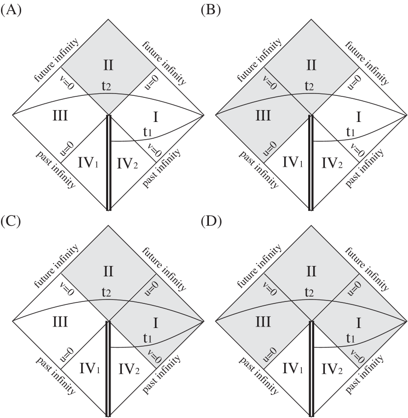
It is easy to know the global structure of the Roberts solution because is the Minkowski spacetime. and are affine parameters along radial null geodesics, and then null infinities are represented by or . The Penrose diagram of the Roberts spacetime for with is given in Fig. 1. This spacetime represents a dynamical wormhole. (Several (quasi-)local definitions of a dynamical wormhole have been independently proposed so far hayward1999 ; hv1998 ; mhc2009 .)

Now we show that the Roberts spacetime can be attached to the Minkowski spacetime at or in a regular manner, i.e., without a massive thin shell on the hypersurface. (See bi1991 ; Poisson for the matching condition on a null hypersurface.) We consider a null hypersurface as a matching surface, which we call . (The argument is similar for .) The induced metric on is given by
| (16) |
where is a set of coordinates on . The basis vectors of defined by are given by
| (17) | ||||
| (18) |
The basis is completed by satisfying and on . The only nonvanishing component of the transverse curvature of is
| (19) |
The regular attachment on requires the continuity of and on both side of . Since there is no in the expressions of and , two Roberts spacetimes with the same nonzero but different can be attached in a regular manner at . Thus, as a special case, the Roberts spacetime (7) with and can be attached to the past Minkowski spacetime at in a regular manner, of which metric is given by Eq. (7) with and . Similarly, it is shown that two Roberts spacetimes with the same nonzero but different can be attached in a regular manner at .
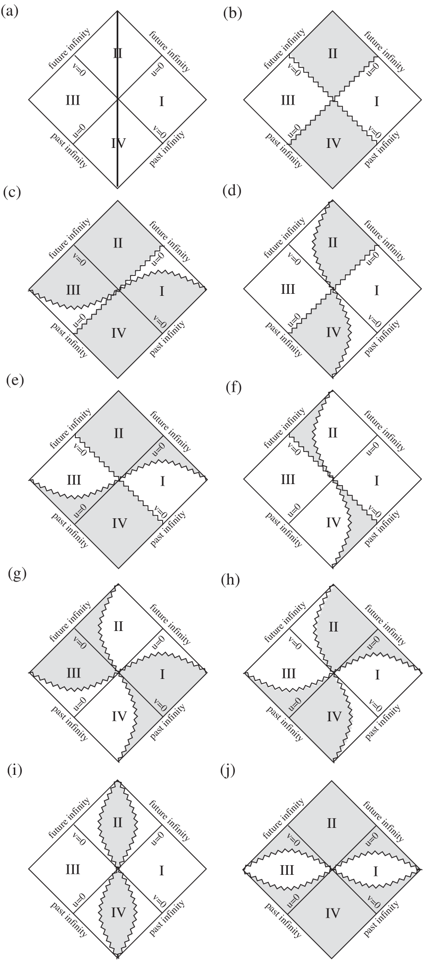
By gluing the Roberts spacetime with , and the Minkowski spacetime(s) at and/or in a regular manner, we can construct spacetimes representing wormhole formation from the initial data with a regular center. The Penrose diagrams for these spacetimes are given in Fig. 2.
The attachment of the Roberts spacetime to the Minkowski spacetime in the case of the ghost scalar field has been mentioned in fj2004 without detailed calculations. It is claimed there that the instantaneous singularity in the Roberts spacetime can be removed by gluing the Minkowski spacetime at or . Obviously, the curvature invariants do not blow up if an observer approaches there from the Minkowski region, however, they certainly blow up along some causal geodesics emanating from in the Roberts region. As a result, there is still a naked singularity at in the resulting spacetime. The details will be presented in the next section.
IV Properties of the instantaneous singularity
In the last section, we constructed a spacetime representing the wormhole formation. One problem in this spacetime is an instantaneous curvature singularity at which appears at the moment of the wormhole formation. In this section, we show that it is a naked but weak singularity.
IV.1 Nakedness
First we show that both radial and nonradial causal geodesics emanate from , i.e., it is certainly a naked singularity. The Lagrangian to give the geodesic equations is
| (20) |
where a dot denotes the derivative with respect to the affine parameter along a geodesic. Because of spherical symmetry, we can set without loss of generality. The metric (7) is independent of , so that from the Lagrange equation
| (21) |
we obtain a conserved quantity along a geodesic as
| (22) |
Then, the geodesic equations (21) are written as
| (23) | ||||
| (24) |
The tangent vector of a nonspacelike geodesic satisfies
| (25) |
where is and for null and timelike geodesics, respectively. This equation is written as
| (26) |
The Roberts spacetime admits a homothetic Killing vector satisfying
| (27) |
Then, we obtain
| (28) |
where we used the fact that is tangent to a geodesic and Eq. (27). Hence we obtain , or equivalently
| (29) |
where is a constant. Equation (29) is integrated to give
| (30) |
where is a constant.
We are now interested in the geodesics emanating from . Without loss of generality, we can set such that corresponds to . Thus, we consider the case with . Now the geodesic equations reduce to
| (31) | ||||
| (32) |
We obtain the master equation for from above equations as
| (33) | ||||
| (34) |
First we consider radial geodesics (). For the null geodesics (), the solutions of Eqs. (31) and (32) passing through are or . Along these radial null geodesics, the Kretschmann invariant and the quasilocal mass are identically zero. For the timelike geodesics (), the general solution of Eq. (33) is given by and , where is a nonzero constant. These two coincide for and the latter does not pass through for . Finally, the solution passing through is given by
| (35) |
which corresponds to in Eq. (32). The Kretschmann invariant along these radial timelike geodesics is given by
| (36) |
which diverges at , i.e., . Along these radial timelike geodesics, the quasilocal mass is given by
| (37) |
which converges to zero at .
For the nonradial geodesics (), there is a solution of Eqs. (31) and (32) passing through , which is given by
| (38) | ||||
| (39) |
Under and , the conditions for and to be real and positive are and
| (40) |
Because and are independent parameters which characterize a geodesic, the right-hand side of Eq. (40) varies from to infinity. Hence, for any values of and satisfying and , there are nonradial causal geodesics passing through .
IV.2 Strength
Next we consider the strength of the singularity at . As definitions of the strength of singularities, the strong curvature condition (SCC) Tipler and the limiting focusing condition (LFC) Krolak were proposed by Tipler and Królak, respectively. We consider a geodesic (N), affinely parametrized by , with the tangent vector , terminating at or emanating from a singularity, where . SCC and LFC imply that N is emanating from or terminating in the Tipler’s strong and the Królak’s strong curvature singularities, respectively ClarkeKrolak . The physical content of the Tipler strong is that the volume element of physical objects (constructed by the Jacobi fields along N) converges to zero at the singularity. On the other hand, the physical content of the Królak strong is that the expansion along N diverges at the singularity, but still the volume element remains finite. (See also Joshi ; Clarketext for the textbook.)
The necessary conditions for SCC and LFC are available ClarkeKrolak . Let a parallelly propagating frame along N satisfying if N is timelike and if N is null. All other products vanish and . If SCC is satisfied along N, then does not converge for and in the cases where N is timelike and null, respectively, where is the Riemann tensor in the parallelly propagating frame. If LFC is satisfied along N, then does not converge for and in the cases where N is timelike and null, respectively.
We show that the singularity at in the Roberts spacetime is weak in the senses of both Tipler and Królak for radial causal geodesics. For the radial causal geodesics, of which tangent vector has the form of , where is satisfied for null geodesics, the angler bases () are given as
| (45) | ||||
| (46) |
which satisfy . The only nonzero component of is
| (47) |
Thus, the only nonzero component of is
| (48) |
These quantities are identically zero both for radial null geodesics ( or ) and radial timelike geodesics (35). Hence, it is concluded that the singularity at is weak in the senses of both Tipler and Królak for radial causal geodesics.
For nonradial geodesics, it seems to be cumbersome to examine . Instead, we here consider the behavior of , which is used in the sufficient conditions for SCC and LFC. SCC is satisfied if and LFC is satisfied if ClarkeKrolak ; Clarketext . The nonzero components of the Ricci tensor of the Roberts spacetime are given by
| (49) | ||||
| (50) | ||||
| (51) |
Finally, for nonradial causal geodesics , where , , and are obtained from (38), (39), and (22), respectively, we obtain , which immediately implies and along the geodesics. Although this result does not directly mean that neither SCC nor LFC is satisfied, it would suggest that the singularity at is weak also along nonradial causal geodesics.
V Summary and discussions
In this paper, we constructed an explicit and simple model of wormhole formation from the initial data with a regular center. The spacetime represents the wormhole formation with a massless ghost scalar field. In this construction, the matter region represented by the Roberts spacetime is attached to the past Minkowski spacetimes at null hypersurfaces in a regular manner.
This construction has been mentioned in fj2004 without a detailed analysis. Actually, unlike the authors’ claim in fj2004 , a naked curvature singularity appears at the moment of the wormhole formation. However, we showed that it is only instantaneous and weak in the senses of both Tipler and Królak. This class of weak singularities could be harmless because it would be dealt with in some distributional sense.
In this context, Hayward and Koyama constructed an analytic model representing the wormhole “formation” from the Schwarzschild black hole kh2004 . Although their model does not contain a singularity at the moment of “formation”, it does not represent the wormhole formation from the initial data with a regular center, i.e., there is no topology change in their model. While they defined a wormhole throat by a class of trapping horizons hayward1999 ; hv1998 , there is a wormhole throat on any spacelike hypersurface in their model. (See mhc2009 for the discussions of the (quasi-)local definition of a wormhole throat on a spacelike hypersurface.)
In the spatially compact spacetime, the wormhole formation necessarily requires the appearance of singularities or closed timelike curves. This is a consequence of the result by Geroch about the topology change of spacetimes geroch1967 . Hence, under the suitable chronology condition, the singularity formation is inevitable. In this paper, on the other hand, the wormhole formation in the spatially noncompact spacetime is considered. The singularity formation would be also inevitable for the wormhole formation in this case, however, as far as the author knows, this is an open question.
The solution presented in this paper will be a simple analytic model to study the formation of a wormhole. In this context, the stability of the wormhole formation is an important future work. While the stability of the Roberts solution was studied in the case of the positive kinetic term of the scalar field frolov1997 , it is still an open question for the ghost scalar field.
Acknowledgments
The author would like to thank T Harada, K. Nakao, J. Oliva, J.M.M. Senovilla, and R. Vera for discussions and comments. The author was supported by Fondecyt Grant No. 1071125. The Centro de Estudios Científicos (CECS) is funded by the Chilean Government through the Millennium Science Initiative and the Centers of Excellence Base Financing Program of Conicyt. CECS is also supported by a group of private companies which at present includes Antofagasta Minerals, Arauco, Empresas CMPC, Indura, Naviera Ultragas, and Telefónica del Sur. The author is also grateful to Universidad del Pais Vasco, Universidade de Santiago de Compostela, and Instituto Superior Técnico for their hospitality during his visit.
Appendix A The relation between the Gutman-Bespal’ko and the Roberts solutions
In 1967, Gutman and Bespal’ko obtained a spherically symmetric solution for a stiff fluid, i.e., a perfect fluid with an equation of state , where and are the pressure and energy density, respectively gb1967 . (See also wesson1978 ; krasinski for the generalized solution.) The energy-momentum tensor for a perfect fluid is given by
| (52) |
where is the four-velocity of the fluid element. The Gutman-Bespal’ko solution is given in the comoving coordinates as
| (53) | |||||
| (54) |
where the constants and satisfy for nonnegative energy density. In the case of , the solution gives the Minkowski solution. The Gutman-Bespal’ko spacetime admits a homothetic Killing vector satisfying .
We show that the Gutman-Bespal’ko spacetime covers half of the Roberts spacetime. In 1988, Madsen showed the equivalence between a massless scalar field and a stiff fluid madsen1988 . This is easily generalized to the ghost case as shown below. The energy-momentum tensor for a stiff fluid is
| (55) |
If is vorticity free, which is satisfied in the spherically symmetric spacetime, one can show that this matter field is equivalent to a massless scalar field , of which gradient is timelike. The corresponding energy density and 4-velocity are given by
| (56) | |||||
| (57) |
with which Eq. (55) coincides with Eq. (2), where the sign in (57) is chosen so that is future-directed.
For the Gutman-Bespal’ko solution, the corresponding scalar field with is
| (58) |
for and
| (59) |
for .
In the Gutman-Bespal’ko spacetime, the metric on is Minkowski in the Rindler coordinates, while it is also Minkowski but in the double null coordinates in the Roberts solution. By the coordinate transformations
| (60) |
of which inverse transformations are
| (61) |
the two-dimensional Rindler metric is transformed into . Adopting the null coordinates such as
| (62) |
we obtain .
Indeed, by the direct transformations
| (63) |
of which inverse is
| (64) |
the Roberts metric (7) is transformed to the Gutman-Bespal’ko metric (53). Therefore, we may call the Gutman-Bespal’ko metric (53) the Rindler chart of the Roberts metric. Because of , the Rindler chart covers only half of the Roberts spacetime. (The regions I and III in Figs. 1 and 3.)
On the other hand, by the coordinate transformations
| (65) |
of which inverse is
| (66) |
the two-dimensional Minkowski spacetime is transformed to the Milne form . Thus, by the direct transformations
| (67) |
of which inverse is
| (68) |
the Roberts solution is transformed to
| (69) | |||||
| (70) |
for . For , the scalar field is transformed to
| (71) |
We may call this metric the Milne chart of the Roberts metric. Because of , the Milne chart covers the regions II and IV in Figs. 1 and 3. This spacetime admits a homothetic Killing vector satisfying .
Appendix B The Roberts solution for
In this appendix, we review the properties of the Roberts spacetime with corresponding to the positive kinetic term of the scalar field. First we see in Eq. (10) that the region with has negative mass. In the case with , , and , there are nonnull central curvature singularities located at
| (72) |
If , both of them are timelike or spacelike, while if , one is spacelike and the other is timelike. For and , there are null and nonnull central curvature singularities at and , respectively. For and , there are null and nonnull central curvature singularities at and , respectively. For and , there are null central curvature singularities at and . The Penrose diagram of the Roberts spacetime for is given in Fig. 3.
As shown in the main text, the Roberts spacetime can be attached to the Minkowski spacetime at a null hypersurface or in a regular manner if that hypersurface is regular. The resulting spacetime can be a model of the gravitational collapse leading to the naked singularity formation. This model has been considered in the context of critical phenomena or cosmic censorship roberts1989 ; brady1994 ; ont1994 ; brady1995 ; frolov1997 ; hayward2000 ; application .
References
- (1) M. Visser, B. Bassett, and S. Liberati, arXiv:gr-qc/9908023; M. Visser, B. Bassett, and S. Liberati, Nucl. Phys. Proc. Suppl. 88, 267 (2000);
- (2) M. Visser, Lorentzian Wormholes: From Einstein to Hawking, (Springer-Verlag, Berlin, Germany, 1997).
- (3) F.S.N. Lobo, e-Print: arXiv:0710.4474 [gr-qc].
- (4) M.S. Morris, K.S. Thorne, and U. Yurtsever, Phys. Rev. Lett. 61, 1446 (1988).
- (5) M. Visser, Phys. Rev. D47, 554 (1993); S.W. Kim and K.S. Thorne, Phys. Rev. D43, 3929 (1991).
- (6) M.S. Morris and K.S. Thorne, Am. J. Phys. 56, 395 (1988).
- (7) H. G. Ellis, J. Math. Phys. 14, 104 (1973); H. G. Ellis, Gen. Rel. Grav. 10, 105 (1979); K. A. Bronnikov, Acta Phys. Polon. B 4, 251 (1973); T. Kodama, Phys. Rev. D 18, 3529 (1978); G. Clément, Gen. Rel. Grav. 13, 763 (1981).
- (8) D. Hochberg and M. Visser, Phys. Rev. D58, 044021 (1998).
- (9) D. Ida and S.A. Hayward, Phys.Lett. A260, 175 (1999); M. Visser, S. Kar, and N. Dadhich, Phys. Rev. Lett. 90, 201102 (2003); C.J. Fewster and T.A. Roman, Phys. Rev. D72, 044023 (2005); P.K.F. Kuhfittig, Phys. Rev. D73, 084014 (2006); O.B. Zaslavskii, Phys. Rev. D76, 044017 (2007).
- (10) J. L. Friedman, K. Schleich, and D. M. Witt, Phys. Rev. Lett. 71, 1486 (1993) [Erratum-ibid. 75, 1872 (1995)]; G. J. Galloway, K. Schleich, D. M. Witt, and E. Woolgar, Phys. Rev. D 60, 104039 (1999).
- (11) A.G. Agnese and M. La Camera, Phys. Rev. D51, 2011 (1995); L. A. Anchordoqui, S. E. Perez Bergliaffa and D. F. Torres, Phys. Rev. D 55, 5226 (1997); K. K. Nandi, B. Bhattacharjee, S. M. K. Alam, and J. Evans, Phys. Rev. D 57, 823 (1998); P. E. Bloomfield, Phys. Rev. D 59, 088501 (1999); K. K. Nandi, Phys. Rev. D 59, 088502 (1999); K. K. Nandi, A. Islam, and J. Evans, Phys. Rev. D 55, 2497 (1997); K.K. Nandi and Y.-Z. Zhang, Phys. Rev. D 70, 044040 (2004); A. Bhadra and K. Sarkar, Mod. Phys. Lett. A20, 1831 (2005); E.F. Eiroa, M.G. Richarte, and C. Simeone, Phys. Lett. A373, 1 (2008).
- (12) D. Hochberg, Phys. Lett. B251, 349 (1990); H. Fukutaka, K. Tanaka and K. Ghoroku, Phys. Lett. B222, 191 (1989); D.H. Coule and K.-i. Maeda, Class. Quant. Grav. 7, 955 (1990); K. Ghoroku and T. Soma, Phys. Rev. D46, 1507 (1992); N. Furey and A. DeBenedictis, Class. Quant. Grav. 22, 313 (2005); F.S.N. Lobo, Class. Quant. Grav. 25, 175006 (2008).
- (13) M. Visser, S. Kar, and N. Dadhich, Phys. Rev. Lett. 90, 201102 (2003).
- (14) E. Poisson and M. Visser, Phys. Rev. D 52, 7318 (1995); M. Ishak and K. Lake, Phys. Rev. D 65, 044011 (2002); E.F. Eiroa and G.E. Romero, Gen. Rel. Grav. 36, 651 (2004); F.S.N. Lobo and P. Crawford, Class. Quant. Grav. 21, 391 (2004); F.S.N. Lobo, Phys. Rev. D 71, 124022 (2005); E.F. Eiroa and C. Simeone, Phys. Rev. D 76, 024021 (2007); E.F. Eiroa, Phys. Rev. D 78, 024018 (2008); J.P.S. Lemos and F.S.N. Lobo, Phys. Rev. D 78, 044030 (2008).
- (15) H.-a. Shinkai and S.A. Hayward, Phys. Rev. D 66, 044005 (2002).
- (16) C. Armendariz-Picon, Phys. Rev. D 65, 104010 (2002).
- (17) J.A. Gonzalez, F.S. Guzman, and O. Sarbach, Class. Quant. Grav. 26, 015010 (2009); Class. Quant. Grav. 26, 015011 (2009).
- (18) K.A. Bronnikov and S. Grinyok, Grav. Cosmol. 7, 297 (2001); K.A. Bronnikov and S.V. Grinyok, Grav. Cosmol. 10, 237 (2004); Grav. Cosmol. 11, 75 (2005).
- (19) C. W. Misner and D. H. Sharp, Phys. Rev. 136, B571 (1964).
- (20) M.D. Roberts, Gen. Rel. Grav. 21, 907 (1989).
- (21) R.A. Sussman, J. Math. Phys. 32, 223 (1991).
- (22) L.M. Burko, Gen. Relat. Grav. 29, 259 (1997).
- (23) P.R. Brady, Class. Quant. Grav. 11, 1255 (1994).
- (24) Y. Oshiro, K. Nakamura, and A. Tomimatsu, Prog. Theor. Phys. 91, 1265 (1994).
- (25) S.A. Hayward, Class. Quant. Grav. 17, 4021 (2000).
- (26) G. Clement and S.A. Hayward, Class. Quant. Grav. 18, 4715 (2001).
- (27) I.I. Gutman and R.M. Bespal’ko, Sbornik Sovrem. Probl. Grav. Tbilissi, 1, 201 (1967).
- (28) M. S. Madsen Class. Quant. Grav. 5, 627 (1988).
- (29) S.A. Hayward, Phys. Rev. D 49, 6467 (1994).
- (30) S.A. Hayward, Int. J. Mod. Phys. D8, 373 (1999).
- (31) D. Hochberg and M. Visser, Phys. Rev. D58, 044021 (1998).
- (32) H. Maeda, T. Harada, and B.J. Carr, e-Print: arXiv:0901.1153 [gr-qc].
- (33) C. Barrabes and W. Israel, Phys. Rev. D 43, 1129 (1991).
- (34) E. Poisson, A Relativist’s Toolkit (Cambridge University Press, Cambridge, England, 2004).
- (35) A. Feinstein and S. Jhingan, Mod. Phys. Lett. A19, 457 (2004).
- (36) F.J. Tipler, Phys. Rev. Lett. A 64, 8 (1977).
- (37) A. Królak, J. Math. Phys. 28, 138 (1987).
- (38) C.J.S. Clarke and K. Królak, J. Geom. Phys. 2, 127 (1985).
- (39) P.S. Joshi, Global Aspects in Gravitation and Cosmology (Oxford University Press, New York, 1993).
- (40) C.J.S. Clarke, The analysis of Space-Time Singularities (Cambridge University Press, Cambridge, 1993).
- (41) S.A. Hayward and H. Koyama, Phys. Rev. D 70, 101502(R) (2004); H. Koyama and S.A. Hayward, Phys. Rev. D 70, 084001 (2004).
- (42) R.P. Geroch, J. Math. Phys. 8, 782 (1967).
- (43) A.V. Frolov, Phys. Rev. D 56, 6433 (1997); Phys. Rev. D 59, 104011 (1999); Phys. Rev. D 61, 084006 (2000).
- (44) P.S. Wesson, J. Math. Phys. 19, 2283 (1978).
- (45) A. Krasiński, Inhomogeneous Cosmological Models (Cambridge University Press, Cambridge, England, 1997).
- (46) P.R. Brady, Phys. Rev. D 51, 4168 (1995).
- (47) A. Ishibashi and A. Hosoya, Phys. Rev. D 60, 104028 (1999); U. Miyamoto and T. Harada, Phys. Rev. D 69, 104005 (2004); T. Harada and H. Maeda, Class. Quant. Grav. 21, 371 (2004).