Magnetic field dependence of the many-electron states in a magnetic quantum dot: The ferromagnetic-antiferromagnetic transition

Abstract

The electron-electron correlations in a many-electron ($N_{e}=1,2,...,5$) quantum dot confined by a parabolic potential is investigated in the presence of a single magnetic ion and a perpendicular magnetic field. We obtained the energy spectrum and calculated the addition energy which exhibits cusps as function of the magnetic field. The vortex properties of the many-particle wave function of the ground state are studied and for large magnetic fields are related to composite fermions. The position of the impurity influences strongly the spin pair correlation function when the external field is large. In small applied magnetic field, the spin exchange energy together with the Zeeman terms leads to a ferromagnetic-antiferromagnetic(FM-AFM) transition. When the magnetic ion is shifted away from the center of the quantum dot a remarkable re-entrant AFM-FM-AFM transition is found as function of the strength of the Coulomb interaction. Thermodynamic quantities as the heat capacity, the magnetization, and the susceptibility are also studied. Cusps in the energy levels show up as peaks in the heat capacity and the susceptibility.

I Introduction.

Magnetic-doped quantum dotsFurdyna have attracted considerable theoretical and experimental interests over the last two decades. Diluted magnetic II-VI and III-V semiconductor (DMS) quantum dots were fabricated with single-electron controlKlein ; Chen . A rich variety of different magnetic and optical properties were discoveredChang ; Govorov ; Archer ; Besombes ; Schmidt ; Worjnar ; Fernandez . In such structures one can explore the physical properties coming from inter-carrier interactions and the interaction of the carriers with the magnetic ion. This system promises to be relevant for future quantum computing devices, where for instance the spin of the magnetic ion is used as a quantum bit. More recently, electrically active devices were fabricated in which a single manganese ion is inserted into a single quantum dot Leger with control of the amount of charge in the quantum dot and consequently the possibility of the control of magnetism of single Mn-doped quantum dots.

Investigation of the exact electronic structure of a two-dimensional quantum dot confined by a parabolic potential containing several electrons and a single magnetic impurity (in this paper $Mn^{2+}$) in the presence of an applied magnetic field is a new topic. In a recent investigationCheng , a three-dimensional (3D) Cd(Mn)Se quantum dot containing several electrons, where only the low-energy levels of the single-electron problem were taken into account, was investigated in the presence of a magnetic field. Here we will extend this work and include all relevant energy levels in order to obtain a convergent solution for the ground state (and also excited spectrum) of the system.

It is known that in the absence of a magnetic ion, an external magnetic field is able to change the spin polarized state of weakly interacting electrons $N_{e}$ in a quantum dot in such a way that in the ground state it maximizes the total spin of the system: i.e. $S=N_{e}/2$. If the inter-particle interaction is strong, even without an applied magnetic field the electrons may already be polarized. However, with increasing magnetic field and in the case the inter-particle interaction is strong, the total spin of the system can be unusually reduced by the magnetic fieldMarteen .

In the present study, we investigate theoretically the few-electron two-dimensional confined quantum dot system that contains a single magnetic ion in the presence of an external magnetic field taking into account a sufficient large number of single-particle orbitals such that numerical “exact” results are obtained. We explore how sensitive the whole system is to the position of the magnetic ion in the quantum dot and to the presence of a magnetic field and investigate the competition between the following three energies: i) the interaction of the magnetic ion with the electrons, ii) the interaction of the magnetic ion with the magnetic field, and iii) the interaction of the external field with the electrons. These terms affect the spin polarization of the $N_{e}$ electrons in the quantum dot.

Explicit studies of a $N_{e}$-correlated-electron system interacting with a single magnetic ion in nonzero magnetic field are very rare in the literature. Recent theoreticalFernandez ; Cheng ; Hawrylak ; NgaTTNguyen and experimental workLeger has focused either on a small number of electrons using the exact diagonalization approach at zero field (Refs.Hawrylak ; NgaTTNguyen ) for a $2$D quantum dot or at nonzero fieldCheng including only the lowest single-particle states for a 3D system or the exciton states relevant for optical spectroscopy of self-assembled magnetic-doped quantum dotsFernandez ; Leger .

Here, we will examine thoroughly the exact properties of the system containing several correlated electrons and a single magnetic impurity in the presence of a magnetic field. In our numerical “exact” diagonalization approach we include an arbitrary number of single-particle states to guarantee the accuracy of our results. We investigate the influence of the strength of the inter-particle interaction and the position of the magnetic ion on the ground state of the system. We predict the interesting phenomenon that the magnetic ion ferromagnetically couples with the electrons in a region below a critical magnetic field and antiferromagnetically with the electrons above this critical field. Thermodynamic properties as magnetization, susceptibility, and the heat capacity are investigated as function of magnetic field and temperature.

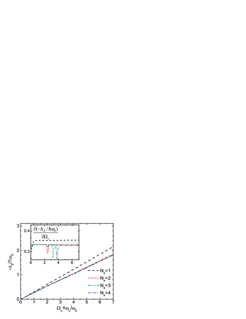
Figure 1: (Color online) Total Zeeman energy for a quantum dot with different number of electrons. The magnetic ion is located at ($0.41l_{0},0$), and the Coulomb interaction strength $\lambda_{C}=0.2$. The inset is the first derivative of $\Delta_{Z}$ with respect to $\Omega_{c}$ that highlights the non-linearity of $\Delta_{Z}$ in certain regions of the magnetic field.

This paper is organized as follows. Section II introduces the model and the numerical method. In section III, we present our numerical results for the many-particle ground state and investigate correlations through the appearance of vortices in the many-electron wave function. Sect. IV addresses the many-particle spectrum and in Sect. V we present results for different thermodynamic quantities. Our discussion and conclusions are presented in Sect. VI.

II Theoretical model

A quantum dot containing $N_{e}$ electrons with spins $\overrightarrow{s_{i}}$ confined by a parabolic potential and interacting with a single magnetic ion ($Mn^{2+}$) with spin $\overrightarrow{M}$ and a magnetic field is described by the following Hamiltonian:

$$\hat{H}=\sum_{i=1}^{N_{e}}\left[\frac{1}{2m^{*}}{\left(-i\hbar\overrightarrow{\nabla}_{\overrightarrow{r}_{i}}+e\overrightarrow{A}(\overrightarrow{r_{i}})\right)^{2}}+\frac{1}{2}{m^{*}\omega_{0}^{2}\overrightarrow{r_{i}}^{2}}\right]+\sum_{i<j=1}^{N_{e}}\frac{e^{2}}{4\pi\epsilon_{0}\epsilon|\overrightarrow{r_{i}}-\overrightarrow{r_{j}}|}$$

$$+\frac{1}{2}\hbar\omega_{c}\left(g_{e}m^{*}{S}_{z}+g_{Mn}m^{*}M_{z}\right)-J_{c}\sum_{i=1}^{N_{e}}\overrightarrow{s_{i}}\cdot\overrightarrow{M}\delta(\overrightarrow{r_{i}}-\overrightarrow{R}).$$ (1)

The vector potential $\overrightarrow{A}$ is taken in the symmetric gauge: $\overrightarrow{A}=B/2(-y,x,0)$ where the magnetic field $\overrightarrow{B}$ points perpendicular to the plane of the interface. The confinement frequency $\omega_{0}$ is related to the confinement length by: $l_{0}=\sqrt{{\hbar}/{m^{*}\omega_{0}}}$. $g_{e}$ and $g_{Mn}$ are the Landé g-factor of the host semiconductor and the magnetic ion, respectively. The dimensionless Coulomb strength is defined as: $\lambda_{C}=l_{0}/a_{B}^{*}$ with $a_{B}^{*}=4\pi\epsilon_{0}\epsilon\hbar^{2}/m^{*}e^{2}$ the effective Bohr radius. The cyclotron frequency is: $\omega_{c}=eB/m^{*}$. $L_{z}$, $S_{z}$, and $M_{z}$ are the projections of the total angular momentum of the electrons, their spins, and the magnetic ion in the direction of the magnetic field. The electrons and the magnetic impurity in the quantum dot interact via the contact exchange interaction with strength $J_{c}$.

We use the set of parametersBesombes ; Hawrylak that is applicable to Cd(Mn)Te which is a II(Mn)VI quantum dot with typical lateral size of about tens of nanometers. The dielectric constant $\epsilon=10.6$, effective mass $m^{*}=0.106m_{0}$, $a_{B}^{*}=52.9$ ${\AA}$, $g_{e}=-1.67$, $g_{Mn}=2.02$, $J_{c}=1.5\times 10^{3}meV{\AA}^{2}$, and $l_{0}$ about tens of nanometers ($\hbar\omega_{0}$ corresponding to tens of $meV$). For example, with $\hbar\omega_{0}=51.32$ $meV$ gives $l_{0}=26.45$ Å.

We rewrite the Hamiltonian in second-quantized form:

$$\hat{H}=\sum_{i,\sigma}E_{i,\sigma}c_{i,\sigma}^{+}c_{i,\sigma}+\frac{1}{2}\sum_{ijkl\sigma\sigma^{{}^{\prime}}}\langle i,j|V_{0}|k,l\rangle c_{i,\sigma}^{+}c_{j,\sigma^{{}^{\prime}}}^{+}c_{k,\sigma_{{}^{\prime}}}c_{l,\sigma}+\frac{1}{2}\hbar\omega_{c}\left(g_{e}m^{*}{S}_{z}+g_{Mn}m^{*}{M}_{z}\right)$$

$$-\sum_{ij}\frac{1}{2}{J_{ij}\left(\overrightarrow{R}\right)}\left[\left(c_{i,\uparrow}^{+}c_{j,\uparrow}-c_{i,\downarrow}^{+}c_{j,\downarrow}\right)M_{z}+c_{i,\uparrow}^{+}c_{j,\downarrow}M^{-}+c_{i,\downarrow}^{+}c_{j,\uparrow}M^{+}\right],$$ (2)

where the first term is the single-particle energies $E_{i,\sigma}$ for an electron in state $i$ with spin $\sigma$ and the second term is the Coulomb interaction. The third term is the electron and magnetic ion Zeeman energy. The last sum is the electron-Mn interaction in which the first term describes the difference between the number of spin up and spin down electrons, and the last two terms describe the energy gained by flipping the electron spin along side with flipping the spin of the magnetic ion. $M_{z},M^{+}$, and $M^{-}$ are the z-projection, raising and lowering operators, respectively, of the magnetic ion spin (we consider $Mn$ ions which have a spin of size $M$=5/2).

The single-particle states in a parabolic confinement potential define a complete basis of Fock-Darwin orbitals $\phi_{nl}\left(\overrightarrow{r}\right)$ and spin functions $\chi_{\sigma}\left(\overrightarrow{s}\right)$:

$$\phi_{nls}\left(\overrightarrow{r},\overrightarrow{s}\right)=\varphi_{nl}\left(\overrightarrow{r}\right)\chi_{\sigma}\left(\overrightarrow{s}\right),$$ (3)

with the Fock-Darwin orbitals:

$$\varphi_{nl}\left(\overrightarrow{r}\right)=\frac{1}{l_{H}}\sqrt{\frac{n!}{\pi\left(n+|l|\right)!}}\left(\frac{r}{l_{H}}\right)^{|l|}e^{-il\theta}e^{-r^{2}/{2l_{H}^{2}}}L_{n}^{|l|}\left(r^{2}/l_{H}^{2}\right).$$ (4)

In Hamiltonian (II), $i$ denotes a set of quantum numbers $\{n,l\}$ with $n,l$ the radial and azimuthal quantum numbers, respectively. The effective length $l_{H}=\sqrt{\hbar/m^{*}\omega_{H}}=l_{0}/\alpha$ in the presence of a magnetic field is defined through the hybrid frequency $\omega_{H}=\omega_{0}\sqrt{1+({{\omega_{c}}/{2\omega_{0}}})^{2}}$ where $\alpha=\sqrt[4]{1+(\omega_{c}/2\omega_{0})^{2}}$. The single-particle orbital energy is given by:

$$E_{i,\sigma}=\hbar\omega_{H}(2n+|l|+1)-\hbar\omega_{c}l/2.$$ (5)

The interaction parameters between the electrons and the magnetic ion in the quantum dot is expressed:

$$J_{ij}(\overrightarrow{R})=J_{c}\varphi_{i}^{*}(\overrightarrow{R})\varphi_{j}(\overrightarrow{R})$$ (6)

as a product of two Fock-Darwin orbitals calculated at the position of the magnetic ion.

We construct the many-particle wave function following the configuration interaction (CI) method.

$$\Psi\left(\overrightarrow{x^{*}_{1}},\overrightarrow{x^{*}_{2}},...,\overrightarrow{x^{*}_{N_{e}}},\overrightarrow{M}\right)=\sum^{N_{C}}_{k=1}C_{k}\Psi_{k},$$ (7)

where $\Psi_{k}$ is the $k$-th state of the non-interacting many electron wave function determined by $N_{e}$ electrons with $N_{e}$ different sets of quantum numbers $\left(n,l,\sigma\right)$ and the single scatterer with one of the six states of the $Mn$. $\overrightarrow{x^{*}_{i}}$=$\left(\overrightarrow{r_{i}},\overrightarrow{s_{i}}\right)$ stands for the coordinates and spin of a single electron. In second quantization representation, the state $\Psi_{k}$, which is a Slater determinant composed of single-electron states, can be translated into a ket vector $|k\rangle$ grouping a total of $N_{e}$ electrons into $N_{\uparrow}$ electrons with z-component of spin up and $N_{\downarrow}=N_{e}-N_{\uparrow}$ electrons with z-component of spin down:

$$\Psi_{k}\Longrightarrow|k\rangle=|c^{+}_{i_{1}\uparrow},c^{+}_{i_{2}\uparrow},...,c^{+}_{i_{N\uparrow}}\rangle|c^{+}_{j_{1}\downarrow},c^{+}_{j_{2}\downarrow},...,c^{+}_{j_{N\downarrow}}\rangle|M_{z}\rangle.$$ (8)

Here $i_{1\uparrow}\div i_{N\uparrow}$ and $j_{1\downarrow}\div j_{N\downarrow}$ are the indices of the single-electron states for which each index is a set of two quantum numbers (radial and azimuthal quantum numbers), as mentioned above.

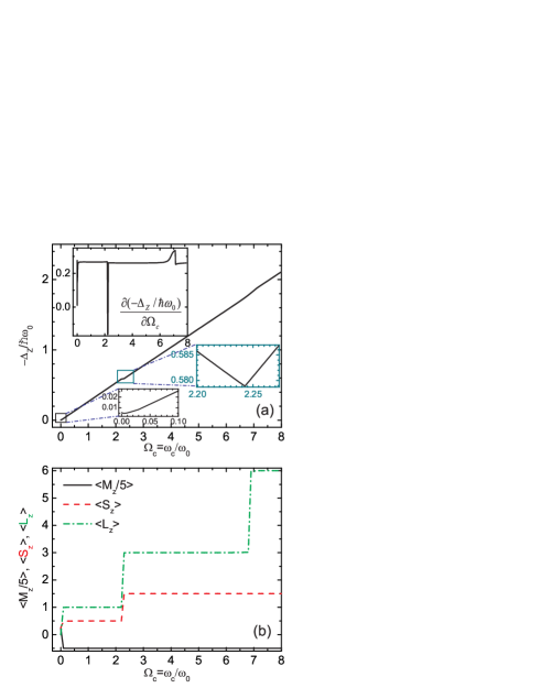
Figure 2: (Color online) Total Zeeman energy (a) calculated for a three-electron quantum dot with the magnetic ion at ($0.5l_{0},0$) and $\lambda_{C}=0.5$. The upper inset is the first derivative of the main plot with respect to $\Omega_{c}$ to visualize more clearly the cusps. The lower inset is a zoom of the rectangular regions of the main plot. (b) The z-projection of the total spin of the magnetic impurity (solid black curve), of the electrons (dashed red curve), and the total angular momentum (dash-dotted green curve).

The CI method, which is in principle exact if a sufficient number of states are included, is limited to a small number of electrons due to computational limitations. For a larger number of electrons and/or magnetic ions, other approaches that e.g. are based on spin-density functional theory (SDFT) using e.g. the local spin density approximation (LSDA) as was used in Ref.Abolfath is able to handle a large number of electrons and/or magnetic ions. The LSDA is exact only in the case of the homogeneous electron gas, and in practice, works well also in most inhomogeneous systems. However, in really highly correlated few-particle systems as discussed in this paper, the LSDA might fail or be at least less accurate.

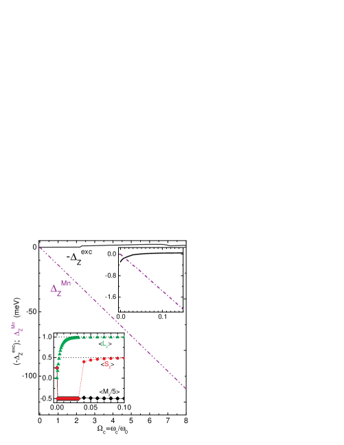
Figure 3: (Color online) Zeeman energy of the magnetic ion and exchange interaction of a three-electron quantum dot with the magnetic ion located at $(0.5l_{0},0)$ and the Coulomb strength $\lambda_{C}=0.5$. The upper inset is a zoom of the small magnetic field region and the lower one presents the average of $M_{z}$, $S_{z}$, and $L_{z}$ for the ground state at very small magnetic fields.

III Ground-state properties

III.1 Zeeman energy

We first explore the magnetic field dependence of the total Zeeman energy:

$$\Delta_{Z}=E_{C}-E_{UC}=\Delta_{Z}^{electron}+\Delta_{Z}^{Mn}+(-\Delta_{Z}^{exc})$$ (9)

which is the difference in energy in the presence and without a magnetic ion. It consists of three terms: the difference of the Zeeman energy of the electrons $\Delta_{Z}^{electron}$, the Zeeman energy describing the interaction of the magnetic ion having spin $\textbf{M}=5/2$ with the magnetic field, $\Delta_{Z}^{Mn}$, and the exchange interaction of the ion with the electrons, $-\Delta_{Z}^{exc}$. $\Delta_{Z}^{exc}$ is just the so called “local Zeeman splitting term” as discussed in Ref.NgaTTNguyen . This sum is basically the difference in the Zeeman energy of the electrons between the cases with and without a magnetic ion plus the energy contribution of the magnetic ion.

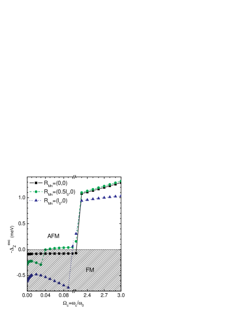
Figure 4: (Color online) Exchange interaction of a three-electron quantum dot with the magnetic ion located at three different positions: $(0,0)$, $(0.5l_{0},0)$, and $(l_{0},0)$ for the Coulomb strength $\lambda_{C}=0.5$. The horizontal line at $\Delta_{Z}^{exc}=0$ separates the $\Delta_{Z}^{exc}$ plane into ferromagnetic (FM) and antiferromagnetic (AFM) regions.

For $N_{e}=1$, we find a total Zeeman energy that appears linear in magnetic field. A similar linear behavior is also found in the cases with $N_{e}>1$ but with different slopes (see Fig. 1). Let us suppose, in Hamiltonian (II), that the contribution from the last term (the local Zeeman energy or the exchange interaction term) is zero. For instance this is the case when a magnetic ion is located at the center of the quantum dot having three-electrons in the partially filled $p$ shell, in which the first two-electrons fully fill the $s$ shell and the remaining one is in either of the orbitals of the $p$ shell. Then a perfect linear behavior of the total Zeeman energy is found.

A closer look to $\Delta_{Z}$ gives us a slightly different picture, as is provided by taking the derivative (see the inset of Fig. 1). Notice that the total Zeeman term $\Delta_{Z}$ has pronounced cusps and the number and positions of these cusps is different for different number of electrons $N_{e}$. There exists one at $\Omega_{c}=2.6$ for a two-electron quantum dot, one at $\Omega_{c}=3.4$ for a three-electron quantum dot, and two at $\Omega_{c}=2.5$ and $3.8$ for the four-electron quantum dot, with the magnetic ion located at $(0.41l_{0},0)$. The three-electron system exhibits a much richer behavior when we increase the Coulomb interaction strength to $\lambda_{C}=0.5$ as seen in Fig. 2(a) where we placed the magnetic ion at $(0.5l_{0},0)$. Cusps, which are highlighted in the two insets in Fig. 2(a), appear when the total angular momentum and/or the total z-projection of the spin of the electrons change abruptly with magnetic field. Notice that the total Zeeman energy of a two-electron quantum dot in the presence of the magnetic ion does not produce a similar behavior due to the fact that the z-projection of the total spin is zero making the main contribution (from the Zeeman spin term of the $Mn$-impurity) negligible.

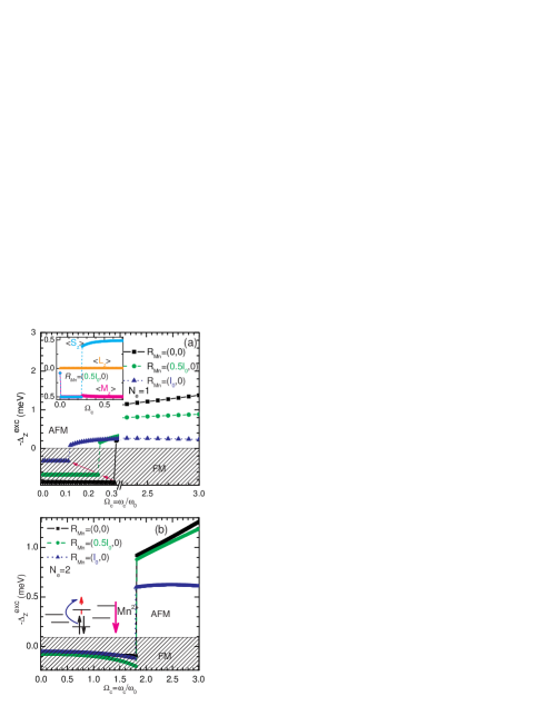
Figure 5: (Color online) Exchange interaction of a one-electron (a) and two-electron (b) quantum dot with the magnetic ion located at three different positions and the Coulomb strength $\lambda_{C}=0.5$. The inset in the upper plot are the averages of the three quantities: $M_{z}$, $S_{z}$, and $L_{z}$ with the ion located at $(0.5l_{0},0)$ at small magnetic fields. The horizontal line separates the plane into ferromagnetic (FM) and antiferromagnetic (AFM) regions in both two plots. The schematic diagram in (b) explains why the exchange energy is almost zero in the case $N_{e}=2$.

The Coulomb strength and the position of the magnetic impurity affects the total Zeeman energy and influences the number and the position of the cusps. The first pronounced cusp appears at lower magnetic field for larger Coulomb interaction strength. This is a consequence of the competition between the Coulomb energy and the energy gap of the single-particle problem. Larger Coulomb strength (smaller energy gap) leads to stronger electron-electron correlation and consequently the electrons are more clearly separated from each other. It results into a high probability for finding the electrons to occupy higher energy states. That also means that the system transfers to a configuration with larger $S_{z}$ and $L_{z}$ at smaller applied field.

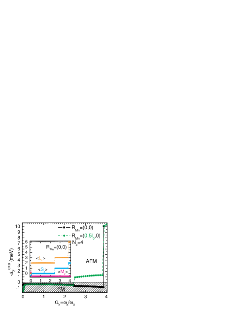
Figure 6: (Color online) Exchange interaction of a four-electron quantum dot with the magnetic ion located at three different positions and the Coulomb strength $\lambda_{C}=0.2$. The horizontal line separates the plane into ferromagnetic (FM) and antiferromagnetic (AFM) regions. The inset shows the total $z$-projection of the $M_{z}$, $S_{z}$, and $L_{z}$ of the electron system with the magnetic ion located at the center of the dot.

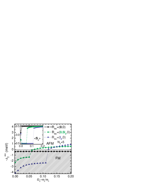
Figure 7: (Color online) Exchange interaction of a five-electron quantum dot with the magnetic ion located at several positions and the Coulomb strength $\lambda_{C}=0.2$. The horizontal line separates the plane into ferromagnetic (FM) and antiferromagnetic (AFM) regions. The inset shows $S_{z}$ alone vs. magnetic field.

We also found that the ground-state energy is sensitive to the presence of the magnetic field. In zero magnetic field, the ground state receives contributions from many different configurations having z-projection of the magnetic ion, $M_{z}$, from $-5/2$ to $5/2$. When a magnetic field is applied, the ground state favors states with projection of the spin of the magnetic ion down and the states with $M_{z}=-5/2$ give the main contribution to the ground state.

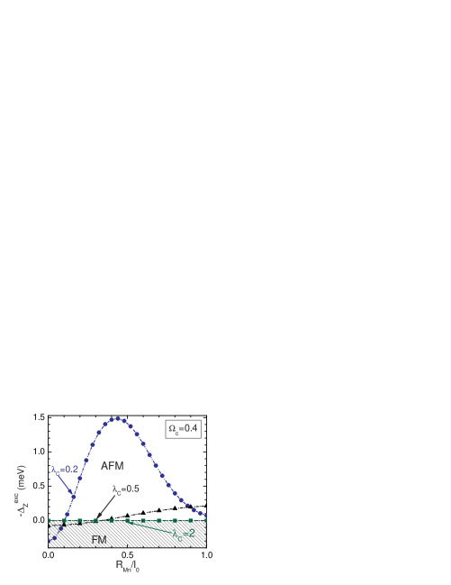
Figure 8: (Color online) The magnetic ion position dependence of the exchange interaction of a three-electron quantum dot for Coulomb strengths $\lambda_{C}=0.2$, $0.5$, and $2$ at $\Omega_{c}=0.4$. The horizontal dotted line at $\Delta_{Z}^{exc}=0$ separates the plane into ferromagnetic (FM) and antiferromagnetic (AFM) regions.

Fig. 2(b) shows the average of the three quantities $M_{z}$, $S_{z}$, and $L_{z}$ of the three-electron quantum dot as a function of the magnetic field for a Coulomb interaction strength $\lambda_{C}=0.5$. We realize that with increasing $\lambda_{C}$ the $<L_{z}>$ ($<S_{z}>$) exhibits jumps at smaller critical $\Omega_{c}$ (compare green dash-dot-dot curve in Fig. 1).

III.2 Antiferromagnetic coupling

Now we direct our attention to the very small magnetic field behavior. There exists a very small region of the magnetic field where the total spin of electrons and the total spin of the magnetic ion are oriented parallel, we found this earlier in Ref.NgaTTNguyen for the zero magnetic field case. These results are now extended to nonzero magnetic field. This is made more clear in the upper inset of Fig. 3 where the crossing point of the two terms: the Zeeman energy of the magnetic ion ($\Delta_{z}^{Mn}$) and the exchange interaction ($\Delta^{exc}_{z}$), occurs at $\Omega_{c}=0.01$ (converted to $B\approx 0.1T$ for the considered system). This ferromagnetic coupling extends further, up to $\Omega_{c}=0.04$ (see the lower inset of Fig. 3).

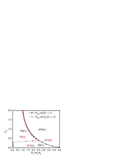
Figure 9: (Color online) Phase diagram for the ferromagnetic-antiferromagnetic transition of a three-electron quantum dot with the magnetic ion located at $(0,0)$ (black squares referred to (1)) and ($2l_{0}=5.29{\AA},0$) (red circles referred to (2)).

It is worth noticing that this ferromagnetic coupling is extended to a much larger magnetic field range (up to $\Omega_{c}=2.3$) if we move the magnetic ion to the center of the quantum dot (see Fig. 4). This can be understood as follows. When the magnetic ion is located at the center of the dot and the magnetic field is very small the absolute value of $\Delta_{z}^{Mn}$ always dominates over $\Delta^{exc}_{z}$. This is opposite to the case when the magnetic ion is located at $(0.5l_{0},0)$. Recall that in Ref.NgaTTNguyen we found for zero field that the exchange Zeeman energy is minimum when the magnetic ion is at the center of the quantum dot and approximately zero at positions very far from the center of the quantum dot.

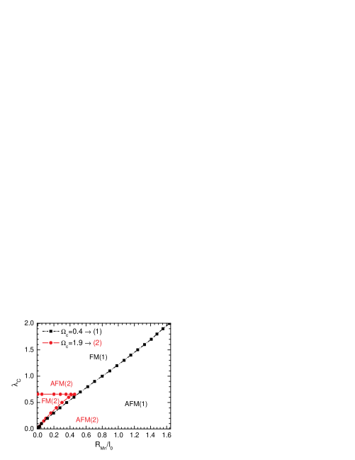
Figure 10: (Color online) Phase diagram for ferro-antiferromagnetic transition of a three-electron quantum dot in an applied field of $\Omega_{c}=0.4$ (black squares referred to (1)) and $\Omega_{c}=1.9$ (red circles referred to (2)).

Fig. 4 tells us that the magnetic field where the antiferromagnetic coupling between electron and the magnetic ion starts depends on the position of the magnetic ion in the quantum dot. The system with the magnetic impurity located at $(l_{0},0)$ exhibits an antiferromagnetic coupling for $\Omega_{c}\geq 0.1$, that is larger than $\Omega_{c}=0.05$ in case of $(0.5l_{0},0)$.

We have discussed the appearance of antiferromagnetism in a three-electron quantum dot. Now we go back to the two simpler cases with the number of electrons $N_{e}=1,2$ (see Fig. 5). Let us first discuss the results for $N_{e}=1$ as given in Fig. 5(a). The antiferromagnetic coupling between the electron and the magnetic ion starts at smaller magnetic field as the magnetic ion is moved. This is different from the previous results for $N_{e}=3$. The reason is as follows: for the quantum dot with a single electron, the electron tends to accommodate permanently the $s$-shell with $<L_{z}>=0$ (see the inset of Fig. 5(a)) in the ground state while the exchange parameter in the $s$ shell ($J_{ss}$) is found to be maximum right at the center of the quantum dot. Moving the magnetic ion away from the center of the dot, this $J_{ss}$ is found to be smaller and as a consequence the exchange electron-$Mn$ interaction becomes smaller than the electron Zeeman energy, leading to an antiferromagnetic coupling at smaller magnetic field.

The story for $N_{e}=2$ electrons (see Fig. 5(b)) is now interesting since the two electrons accommodate the $s$ shell with spins antiparallel making the total spin of the electron zero in the ground state with almost unit probability. This leads to zero contribution to the first term written in the last line in [II] for diagonal elements. Therefore, the main contribution (even very small) to the exchange energy is now expected to come from coupling with configurations where one of the electrons (spin down) stays in the $s$ level and the other occupies higher level (see the schematic diagram in Fig. 5(b)). In this diagram, the magnetic ion is assumed to be located at the center of the dot with spin down ($-5/2$). The coupling of the electron (spin up) in the $s$ orbital with an electron from either of the $p$ shell is zero. The only non-zero coupling is with an electron with the quantum numbers (1,0) of the $d$ shell (as shown in the diagram and this quantum state would change if the ion is located away from the center of the dot) with the amount of about $-10^{-2}$. This picture remains valid until the magnetic field is high enough to excite one electron from the $s$ shell to a higher quantum state forming the ground state with two up spins antiferromagnetically coupling with the magnetic ion. For smaller Coulomb interaction strength, the antiferromagnetic behavior occurs at larger magnetic field since the two electrons repel each other less and consequently they stay longer antiparallel in the $s$ shell.

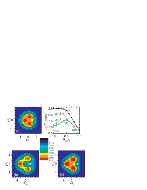
Figure 11: (Color online) Radial density scaled by $l_{0}^{2}$ calculated for a three-electron quantum dot with the magnetic ion (white cross) located at $(0.5l_{0},0)$ in (a), (b) and $(0.8l_{0},0)$ in (c) when the Coulomb strength $\lambda_{C}=0.5$ in a magnetic field $\Omega_{c}=6.4$ (see (a)) and $\Omega_{c}=7$ (see (b) and (c)). (d) is the magnetic ion position dependence of $-\Delta_{Z}^{exc}$ with the magenta circles indicating the respective calculated positions of the magnetic ion in (a), (b), and (c). Red color region is for highest value of radial density.

From the $N_{e}=2$ result we may ask a question: whether a four-electron quantum dot has similar properties since the number of electrons in both cases are even and one may have a situation where the total spin of the electrons is zero. Indeed, if the magnetic ion is located at the center of the quantum dot even though for $N_{e}=4$ the outer shell is half-filled, this is possible as illustrated in Fig. 6 where the antiferromagnetic coupling occurs at $\Omega_{c}=3.87$ at which the total spin of the electrons reaches the maximum value $<S_{z}>=2$. In this case, the first two electrons will occupy the $s$ shell and the remaining two will occupy two of the five orbitals of the $p$ and $d$ shells. This picture holds at small magnetic field. However, there is a big difference in the exchange energy as compared to the previous case of $N_{e}=2$ when the ion is shifted away from the center of the dot, e.g. in this plot at $(0.5l_{0},0)$. The exchange energy is much larger than the result obtained for $R_{Mn}=(0,0)$ because when the ion is out of the center of the quantum dot, the two remaining electrons at higher orbitals have a non-zero contribution in the diagonal exchange elements dominating the exchange energy of the ground state. This is the reason why the antiferromagnetic transition occurs at smaller magnetic field ($\Omega_{c}=2.5$) as compared to the case when the ion is at the center of the dot ($\Omega_{c}=3.87$) although the pictures of the $M_{z}$ and $L_{z}$ transition in these cases are similar.

To complete the picture for few-electron quantum dot system, we will discuss the AFM behavior for the system with the highest number of electrons, $N_{e}=5$, where we were able to obtain accurate numerical results. We focus on the small magnetic field region (see Fig. 7). For the magnetic ion in the center of the dot, the FM coupling is dominant in the shown magnetic field region because the diagonal exchange matrix elements dominate over the Zeeman energies of the electrons and of the magnetic ion. This is different for the cases with the magnetic ion displaced a bit from the center of the quantum dot. The FM-AFM occurs at $\Omega_{c}=0.07$ and $\Omega_{c}=0.12$ for $R_{Mn}=(0.5l_{0},0)$ and $R_{Mn}=(l_{0},0)$, respectively. It is similar to the cases for the system with $N_{e}=1,3$ due to the zero coupling between the orbitals from the $p,d$ shell with the $s$ orbital. To observe the AFM behavior for the system with the magnetic ion located at the center of the dot where the diagonal exchange elements are almost zero, it is crucial to include enough quantum orbitals (that rapidly increases the size of the Hamiltonian matrix resulting in very time consuming calculations) so that one allows the electrons to jump to higher energy levels and having parallel spins as previously shown for the case $N_{e}=4$ (see Fig. 6). In that case, the four-electron system exhibits an anti-ferromagnetic coupling with the magnetic ion at the magnetic field where the total $z$-projection of the spin is maximum $S_{z}=2$. The system is strongly polarized. For the case $N_{e}=5$, up to $\Omega_{c}=0.2$, the total $S_{z}=0.5$ and the total $L_{z}=1$. The inset in Fig. 7 supports the AFM behavior for the out of center $Mn$ as obtained in the main plot.

III.3 Phase diagram for the ferromagnetic-antiferromagnetic transition

Now we change the Coulomb interaction strength and explore the magnetic behavior as function of the position of the magnetic ion. From Fig. 8, it is clear that when reducing the Coulomb interaction the system undergoes a ferromagnetic to antiferromagnetic transition at gradually larger magnetic fields for $Mn^{2+}$ positions that are closer to the center of the dot. We see that $-\Delta_{Z}^{exc}$ has a peak structure with a maximum at some specific position of the magnetic ion, e.g. see the peak for the case $\lambda_{C}=0.2$ (the blue full circles). However, it is certain that at high magnetic field, the system is always antiferromagnetic.

The FM-AFM phase diagram for a three-electron quantum dot in ($\lambda_{C},\Omega_{c}$) space is shown in Fig. 9 for two different positions of the magnetic ion. When the magnetic ion is in the center of the quantum dot (black curve with squares in Fig. 9) the critical magnetic field increases as the Coulomb interaction strength decreases. The reason is that increasing the Coulomb interaction helps the electrons to approach closer the magnetic ion and therefore the critical magnetic field for the system to transit to the antiferromagnetic phase decreases.

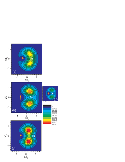
Figure 12: (Color online) Spin up-up pair correlation functions scaled by $l_{0}^{4}$ calculated for the quantum dot of Fig. 11 where one electron (orange arrow) is pinned at one of the three most-probable positions of the electrons as obtained in Fig. 11. It is at $(-0.44l_{0},0)$ in (a) for Fig. 11(a), $(-0.63l_{0},0)$ in (b) for Fig. 11(b), and $(-0.52l_{0},0)$ in (c) for Fig. 11(c), respectively. (b’) The same correlation function for the case the position of the fixed electron is closer to the ion (at $(-0.3l_{0},0)$) as compared to (b). The position of the magnetic ion is indicated by the white cross.

Now we move the magnetic ion away from the center of the quantum dot and we obtain the phase diagram as shown by the red curve (with solid circles) in Fig. 9. For $\lambda_{C}<0.4$, the stability of the FM phase with respect to an applied magnetic field is strongly reduced and a small magnetic field turns the three-electron system into the AFM phase. Notice that for sufficient strong electron-electron interaction (i.e. $\lambda_{C}\geq 0.4$) we obtain practically the same FM-AFM phase diagram as for the case the $Mn$-ion is located in the center of the quantum dot. A remarkable re-entrant behavior is found in the region $0.3<\lambda_{C}<2$ and $0.9<\Omega_{c}<2.5$ where with increasing $\lambda_{C}$ we go from an antiferromagnetic to ferromagnetic and back to antiferromagnetic phase. This unusual behavior is understood as follows. As the impurity is moved away from the center of the quantum dot the exchange matrix will have many nonzero off-diagonal terms that leads to a smaller FM-AFM critical transition magnetic field. Now let us turn our attention to the region $\lambda_{C}<0.4$. For very small Coulomb interaction strength the electrons will repel each other only weakly and are therefore pulled towards the magnetic ion (the nonzero exchange matrix elements increase strongly) resulting in a very small FM-AFM magnetic field. For $\lambda_{C}\geq 0.4$, the electrons become more strongly correlated and the critical field stays about $\Delta\Omega_{c}\approx 0.02\div 0.07$ from the result for $R_{Mn}=0$. If one moves the ion further and further away from the center, the $\lambda_{C}\sim 0.4$ transition line moves to larger $\lambda_{C}$ values. For example, for $\lambda_{C}=0.5$ and the magnetic ion located at $(0.5l_{0},0)$ the FM-AFM critical transition occurs at $\Omega_{c}=0.08$, which is much smaller than $2.21$ found for $R_{Mn}=(0.2l_{0},0)$.

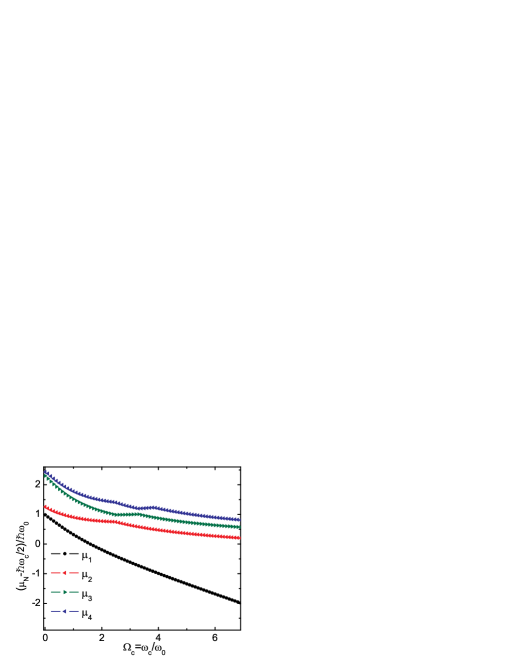
Figure 13: (Color online) Addition energy for different number of electrons. The magnetic ion is located at $(0.41l_{0},0)$ and the Coulomb interaction strength is $\lambda_{C}=0.2$.

The dependence of the ferromagnetic-antiferromagnetic transition of a three-electron quantum dot system on the position of the magnetic ion is summarized in the phase diagram shown in Fig. 10 for two different magnetic fields $\Omega_{c}=0.4,1.9$. We can predict that with slightly larger (smaller) magnetic field the slope of the curve will be larger (smaller). From Fig. 9, we already learned that the FM-AFM transition magnetic field is largest for the ion in the center of the quantum dot as is also seen in Fig. 10. The re-entrant behavior of the AFM phase as function of $\lambda_{C}$ is found for small $R_{Mn}/l_{0}$ values, i.e. when the $Mn$-ion is not too far from the center of the quantum dot, in case the magnetic field is not too small. The critical point ($R_{Mn}/l_{0},\lambda_{C}$)=($0.457,0.656$) for $\Omega_{c}=1.9$ moves down (up) with increasing (decreasing) magnetic field.

III.4 Density and correlation

In high magnetic field, the magnetic ion tends to attract electrons because they are oppositely polarized. Because the exchange interaction is small as compared to the Coulomb interaction, the electrons and magnetic ion are arranged in such a way that the electrons repel each other and also try to be as close to the magnetic ion as possible. This picture holds above the FM-AFM critical magnetic field.

To show this behavior explicitly, we studied the radial density and the radial pair correlation functions. Their respective operators are defined as:

$$\rho(\overrightarrow{r})=\sum_{i=1}^{N_{e}}\delta\left(\overrightarrow{r}-\overrightarrow{r_{i}}\right),$$ (10)

and

$$C_{\sigma\sigma^{{}^{\prime}}}(\overrightarrow{r},\overrightarrow{r}^{{}^{\prime}})=\sum_{i\neq j}^{N_{e}}\delta_{\sigma\sigma_{i}}\delta\left(\overrightarrow{r}-\overrightarrow{r_{i}}\right)\delta_{\sigma^{{}^{\prime}}\sigma_{j}}\delta\left(\overrightarrow{r}^{{}^{\prime}}-\overrightarrow{r_{j}}\right).$$ (11)

We plot in Fig. 11 the radial density of a three electron quantum dot that is polarized in high magnetic field for the case that the Coulomb strength is $\lambda_{C}=0.5$ and the magnetic ion is located at two different positions for two magnetic fields. The electrons and the magnetic ion are antiferromagnetically coupled. The strength of that coupling can be seen from Fig. 11(d) in which we plot the magnetic ion’s position dependence of the exchange energy at two magnetic fields $\Omega_{c}=6.4,$ and $7$. Those magnetic fields are typical in the sense that the exchange term is found to be very large ($\Omega_{c}=6.4$) or the correlation between the electrons very high ($\Omega_{c}=7$). Density plots are shown for $R_{Mn}$ at $(0.5l_{0},0)$ and ($0.8l_{0},0$). We observe three distinct peaks of maximum probability. They are found at: $(-0.44l_{0},0)$, $(0.22,0.44)l_{0}$, and $(0.22,-0.44)l_{0}$ in Fig. 11(a); $(-0.63l_{0},0)$, $(0.26,0.63)l_{0}$, and $(0.26,-0.63)l_{0}$ in Fig. 11(b); $(-0.52l_{0},0)$, $(0.26,0.52)l_{0}$, and $(0.26,-0.52)l_{0}$ in Fig. 11(c). These figures show clearly the interplay effect where the three electrons on the one hand try to be close to the magnetic ion and on the other hand repel each other via the Coulomb potential energy. It results in the merging of the radial density such that the higher the exchange energy the larger the merging of the local maxima in the electron density and the smaller the correlations. Fig. 11(d) gives an idea about the variation of $-\Delta_{Z}^{exc}$ with the position of the magnetic ion and reaches a maximum at $(0.5l_{0},0)$ for $\Omega_{c}=7$. In Fig. 11(c), the three electrons are less attracted to the magnetic ion via the antiferromagnetic coupling as compared to that in Fig. 11(b). This is due to the fact that the $-\Delta_{Z}^{exc}$ for the case shown in Fig. 11(b) is larger than that in Fig. 11(c). The electrons are therefore found more correlated in the latter case presented by the extended red region in Fig. 11(c). Thereby, correlation between electrons in Fig. 11(c) is expected to be the highest and in Fig. 11(a) the smallest.

The position of the magnetic ion affects the ground-state property as is made clear in Fig. 12. We fix the spin state and the position of one electron (indicated by the orange arrow) and the position of the magnetic ion (the white cross). The magnetic field is such that $\Omega_{c}=6.4$ in Fig. 12(a) and $\Omega_{c}=7$ in the others. It also reflects the fact that the system in Fig. 11(a) exhibits the smallest correlation as compared to the other two. This illustrates the point raised above about the density. At the magnetic field $\Omega_{c}=7$, the electrons are strongly polarized resulting in the red regions of the up-up spin pair correlation function that tends to surround the magnetic ion. We see that the three electrons are most likely to localize around some specific positions defining a triangle with the three electrons at the three vertices, while they are attracted to the magnetic ion. When we locate one electron at a position closer to the magnetic ion, see Fig. 12(b’), the two peaks decrease in amplitude as compared to those in Fig. 12(b).

III.5 Addition energy

The addition energy (often called the chemical potential) is defined as the increase of the energy of the quantum dot system when an electron is added: $\mu_{N_{e}}=E_{GS}(N_{e})-E_{GS}(N_{e}-1)$. This quantity can be measured experimentally and is plotted in Fig. 13 as function of the magnetic field.

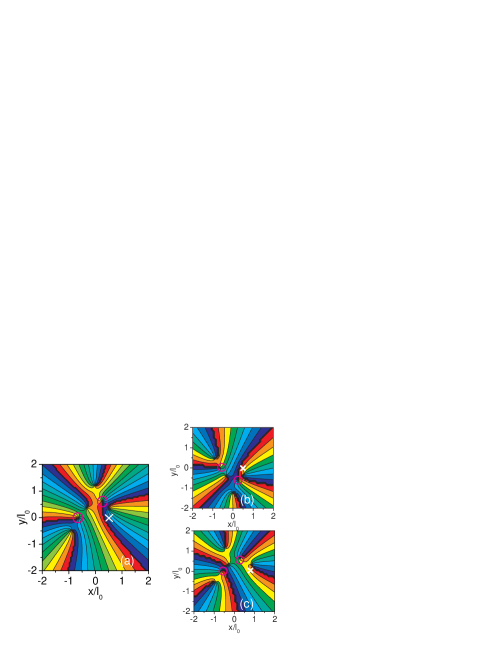
Figure 14: (Color online) Contour plot for the phase of the reduced wave function of a three-electron quantum dot in magnetic field $\Omega_{c}=11$ with the magnetic ion (the white cross) located at $(0.5l_{0},0)$ in (a),(b) and at $(0.8l_{0},0)$ in (c) for Coulomb strength $\lambda_{C}=0.5$. Two fixed electrons (indicated by the two magenta circles) are located at the two peaks appearing in the radial density: $(-0.63l_{0},0)$ and $(0.26,0.63)l_{0}$ in (a), (c); and $(-0.63l_{0},0)$ and $(0.26,-0.63)l_{0}$ in (b).

There are several cusps appearing in the addition energy curves as a consequence of changes in the ground state. These changes are due to variations in the z-projection of the total spin of the electrons and/or the z-projection of the total angular momentum of the system when the magnetic field increases beyond some specific values. The presence of the magnetic ion leads to more cusps and the position of these cusps is also influenced by the number of electrons and the position of the magnetic ion. The cusps are from either of the two systems in the study. For instance, the green triangles in Fig. 13 are for $\mu_{3}=E_{GS}(N_{e}=3)-E_{GS}(N_{e}=2)$ has two cusps at $\Omega_{c}=2.6$ and $\Omega_{c}=3.4$. The cusp at the point $\Omega_{c}=2.6$ comes from the change in the configuration of the average of the total z-projection spin and the total z-projection of angular momentum $(S_{z},L_{z})$ of the two-electrons in the quantum dot from (0,0) to (1,1). While the other cusp $\Omega_{c}=3.4$ comes from the change of the phase of the three-electron quantum dot from $(0.5,1)$ to $(1.5,3)$. It is similar to the case for $\mu_{4}$ (the blue left pointing triangles) where the cusp appears at $\Omega_{c}=3.4$. At this point, we observed a change from configuration ($0,2$) to ($1,3$). The remaining one, $\Omega_{c}=3.9$, is from the four-electron case when its configuration changes from ($1,3$) to ($2,6$).

III.6 Vortex structure: many-body correlations

Another way to obtain information on the correlations that are present in the many-particle wave function is to investigate the vortex structure. At a vortex the many-body wave function is zero and is characterized by a change of phase of $2\pi$ when we go around this point.

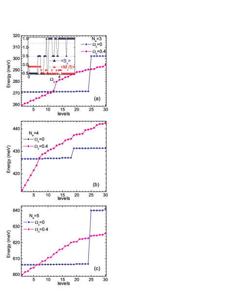
Figure 15: (Color online) The energy spectrum of the first $30$ levels of the three (the top), four (the middle), and five (the bottom) electron quantum dot with the magnetic impurity located at $(0.5l_{0},0)$. The Coulomb strength is $\lambda_{C}=0.5$ with magnetic fields $\Omega_{c}=0.0$ (the blue squares) and $\Omega_{c}=0.4$ (the magenta circles). The inset in the top figure shows the average of $M_{z}$ (the dark-blue triangles) and $S_{z}$ (the red triangles) as a function of $\Omega_{c}$ of the sixth energy level.

The zeros of the wave function are similar to flux quanta when e.g. the wave function corresponds to the order parameter in a superconductor. The fixed electrons and the zero of the wave function follows closely the displaced electron and one may say that the electron plus its zero form a composite-fermion object. The composite-fermionJKJain ; Saarikoski ; Marteen (and references therein) is a collective quasi-particle that consists of one electron bound to an even number of vortices (flux quanta). The composite-fermion concept introduces a new type of quasi-particle that is used to understand the fractional quantum Hall effect in terms of the integer quantum Hall effect of these composite fermions.

To obtain the zeros of the wave function of the system with $N_{e}$ electrons, we fix $N_{e}-1$ electrons at some positions inside the quantum dot and leave the remaining one free. The resulting reduced wave function gives the probability to find the remaining electrons at different positions in the quantum dot and the zeros’ of this function are those points where the phase of the wave function changes by $2\pi$. As an example, we investigate the situation of a three-electron quantum dot.

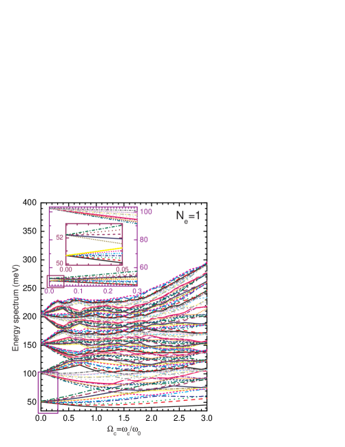
Figure 16: (Color online) The magnetic field dependence of the energy spectrum (the first $120$ levels are shown) of the one-electron quantum dot with the magnetic impurity located at $(0.5l_{0},0)$ and $\lambda_{C}=0.5$ (the inset is a zoom of the first $24$ levels at low magnetic fields and the inset in the inset shows the first $12$ levels, it is a zoom of the rectangular region.

Figs. 14 shows the vortex pictures of a three-electron quantum dot containing a magnetic ion located at positions (see the white cross) that are identical to its positions in Fig. 11(a). Two, among three, electrons are fixed at the respective peaks in the electron density. Red and black regions are referring to the highest (2$\pi$) and lowest phase $0$, respectively. Those plots show that there are always two vortices near the pinned electrons’ positions. For example, the number of vortices pinned to each electron in the case $N_{e}=3$ at $\Omega_{c}=11$ is $2$ describing the system at filling factor $\nu=\frac{N_{e}(N_{e}-1)}{2<L_{z}>}\approx 1/3$. Notice also that one of the vortices appears to be pinned at a position very close to the $Mn$ ion.

We realize that moving the magnetic impurity to a different position changes the relative positions of the vortices that are pinned to the electrons with respect to one another, as shown in Figs. 14(a) and (c). As the electrons are antiferromagnetically coupling to the magnetic ion this kind of movement consequently depends on the position of the magnetic ion.

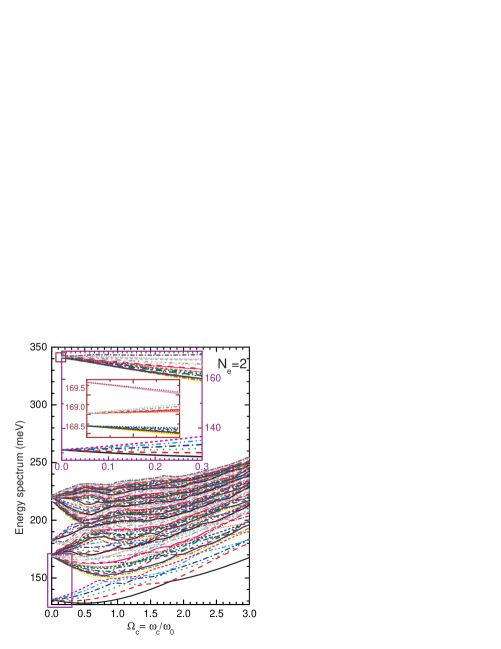
Figure 17: (Color online) The same as Fig. 16 but now for the two-electron quantum dot. The inset in the inset is a zoom of levels $7$th to $24$th for magnetic field close to zero.

In the case $\lambda_{C}=0.5$, we found that the average of the maximum z-projection of the total angular momentum is $<L_{z}>=9$ and the two vortices appear at the external field $\Omega_{c}=3.0$. Apparently, the larger $\lambda_{C}$ the smaller $\Omega_{c}$ for which the first two vortices appear at the pinned electrons.

IV Energy spectrum

In the presence of an external magnetic field, the many-fold degeneracy of the energy spectrum of the system is lifted. Fig. 15(a) illustrates that point for the case of three electrons. In the absence of the interaction between the electrons and the magnetic ion and in the absence of a magnetic field (blue squares), the energy spectrum is $7$-fold degenerate for the first $7$ lowest energy levels, the next level is then $5$-fold degenerate, and the next $7$-fold degenerate, and so on. The origin of this was explained in Ref.NgaTTNguyen and is due to the coupling of the electrons and the magnetic ion. When the magnetic field is different from zero, see red circles in Fig. 15, the degeneracy is lifted. In the inset of Fig. 15 we plot $<M_{z}>$ (the magenta triangles) and $<S_{z}>$ (the dark-blue ones) as a function of magnetic field for the sixth level. The average of $<M_{z}>$ and $<S_{z}>$ change abruptly as compared to those found for the ground-state energy, e.g. see Fig. 2. $M_{z}$ and $<S_{z}>$ of the sixth state jump between two different values, e.g. $-1.5$ and $-2.5$ for $<M_{z}>$ and $0.5$ and $1.5$ for $<S_{z}>$ as function of the field. This is a consequence of anti-crossings of energy levels as will be apparent later. The result for four- and five-electron quantum dots are also shown in Fig. 15. We see the degeneracy of $8$, $6$, $4$, and $12$ for the first $30$ levels in the case $N_{e}=4$ and of $7$, $5$, $7$, $5$, $5$, and level $30$ has the same degeneracy with the next energy level beyond the first $30$ for the case $N_{e}=5$ in $B=0$ Tesla.

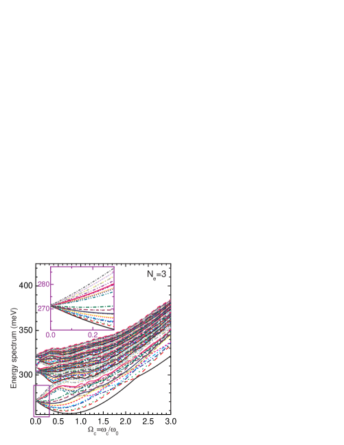
Figure 18: (Color online) The same as Fig. 16 but now for the three-electron quantum dot.

To have a clearer picture of the energy spectrum of the quantum dot system we plot in Figs. 16, 17, and  18 the magnetic field dependence of the first $120$ energy levels for $N_{e}=1,2,3$, respectively. The spectra at small magnetic fields is enlarged (see insets) to see the Zeeman splitting and the nearly-linear behavior of the energy levels. Remember that this is due to the coupling of the electron spins with the magnetic ion spin. For $N_{e}=1$ the first two levels for $B=0$ are $7$- and $5$-fold degenerate ($7$-fold degenerate is due to the ferromagnetic coupling of the $s$-shell electron spin $1/2$ with the magnetic ion spin $5/2$ and $5$-fold degenerate of that electron now with spin $-1/2$ to the magnetic ion with spin $5/2$), respectively. A closer inspection (see Fig. 16) tells us that these $12$-levels are exchange split into two bundles of $7$- and $5$-levels (the inset in the inset in Fig. 16). Notice that there is a first large energy gap at very small fields between the first $12$ levels and the next $24$ ones as seen in Fig. 16 while that kind of gap appears between the first $6$ and the next $36$ for $N_{e}=2$ (Fig. 17). For $N_{e}=3$ (Fig. 18), this kind of gap appears after the first $24$ energy levels. The origin is the coupling of the third electron, which can reside at either two states of the $p$ shell while the $s$ shell is already fully filled, with the magnetic ion with $6$ $z$-components of the spin at very small fields, i.e. the intra-shell ($p$) exchange interaction. For $N_{e}=2$ the electron ground state corresponds with a filled $s$-shell, i.e. $<S_{z}>=0$, and therefor for $B=0$ only a $6$-fold degeneracy, as shown in Fig. 17, is found due to the $z$-component of the $Mn$-spin. The next level is $8$-fold degenerate at $B=0$ ($8$ come from the ferromagnetic coupling of the two-electron system with total spin $1$ to the magnetic ion with spin $5/2$) (see the inset in the inset in Fig. 17), etc.

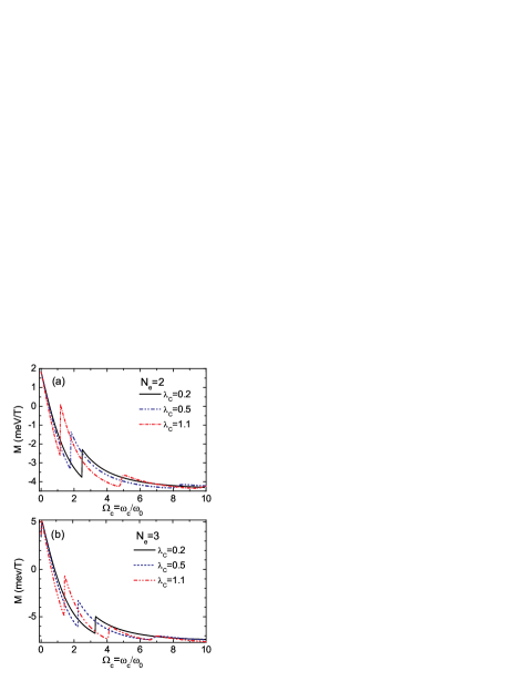
Figure 19: (Color online) Magnetization of the ground state of the two- and three-electron quantum dot with the magnetic ion located at $(0.5l_{0},0)$ for three values of the Coulomb strength $\lambda_{C}=0.2$, $0.5$, and $1.1$.

With increasing magnetic field, we see that for $N_{e}=1$ there is periodically an opening of energy gaps in the spectrum. Similar energy gaps have been found earlier (as an example see e.g Ref.Tarucha ) for a quantum dot without a magnetic impurity and are a consequence of the electron with two-fold spin degeneracy filling the equally-gaped-energy single-particle quantum states with different sets of the radial and angular quantum numbers. Notice that for $N_{e}=2,3$, these gaps have disappeared.

Figure 20: (Color online) Temperature dependence of the magnetization and susceptibility for a three-electron quantum dot with the magnetic ion located at $(0.5l_{0},0)$ and $\lambda_{C}=0.2$.

The spectra exhibit a lot of crossings and anti-crossings, the number of them has increased as compared to the quantum dot case without a magnetic ion because of the Zeeman splitting of the $Mn$-spin. When the applied field increases the gaps in the spectrum of $N_{e}=1$ are still open and appear more often than in the cases of $N_{e}=2,3$. Once again, we see a lot of cusps in the energy levels and that reminds us to abrupt changes in the configuration of the system with magnetic field as discussed before for the ground state.

V Thermodynamic properties

V.1 Magnetization and susceptibility

We first calculate the magnetization and susceptibility of the system: $M=-\partial E_{GS}/\partial B$ and $\chi=\partial{M}/\partial{B}$ at zero temperature.

The magnetization of a quantum dot with the magnetic ion located at $(0.5l_{0},0)$ with $N_{e}=2,3$ electrons is plotted in Fig. 19. We see several jumps that are a consequence of changes in the ground state, e.g. changes in $<L_{z}>$ (see previous section). For example, the magnetization of the three-electron quantum dot as plotted in Fig. 19(b) for the case $\lambda_{C}=0.2$ and the magnetic ion at $(0.5l_{0},0)$ has a step at $\Omega_{c}=3.3$. Consequently, the susceptibility also has a peak at $\Omega_{c}=3.3$. The same thing happens at $\Omega_{c}=1.4,4.1,$ and $6.8$ for $\lambda_{C}=1.1$ in the magnetization and the susceptibility.

For non-zero temperature, the temperature dependence of the magnetization and susceptibility is defined by: $M(T)=-\partial\langle E(T)\rangle/\partial B$, $\chi(T)=\partial M(T)/\partial B$, respectively. The statistical average $<E(T)>$ is calculated as:

$$\langle{E\left(\lambda,T,R_{Mn}\right)\rangle}=\frac{\sum_{{\alpha}=1}^{N_{\alpha}}{E_{\alpha}e^{-E_{\alpha}/k_{B}T}}}{\sum_{{\alpha=1}}^{N_{\alpha}}{e^{-E_{\alpha}/k_{B}T}}},$$ (12)

where the sum is over the energy levels as displayed in e.g. Fig. 15.

These quantities are explored in Figs. 20 for $N_{e}=3$ and a few different temperatures (including the zero temperature case). With increasing temperature the jumps become smoother. A very low magnetic field peak shows up because for $T\neq 0$ we have $M\approx 0$ at $\Omega_{c}=0$.

V.2 Heat capacity

An important quantity that is related to the storage of energy is the heat capacity:

$$C_{V}\left(\lambda,T,R_{Mn}\right)=\frac{\partial{\langle{E\left(\lambda,T,R_{Mn}\right)\rangle}}}{\partial{T}}$$ (13)

The heat capacity is investigated as a function of the Coulomb strength $\lambda$, temperature $T$, magnetic field, and the position of the impurity $R_{Mn}$.

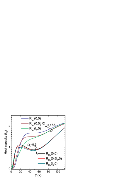
Figure 21: (Color online) The heat capacity vs temperature of a three-electron quantum dot with the magnetic ion located at three different positions, the Coulomb interaction strength is $1.0$ and the magnetic field $\Omega_{c}=0.5$ (the three lower curves) and $7.5$ (the three upper curves).

We plot in Fig. 21 the specific heat for two values of the magnetic field, i.e. $\Omega_{c}=0.5$ and $\Omega_{c}=7.5$, and three typical positions of the magnetic ion. For weak fields, the three electrons start to polarize and we see that the position of the main peak moves towards higher temperature as the magnetic ion is moved away but not too far from the center of the dot. For the high magnetic field case the three electrons are strongly polarized and we see a different behavior in the shift of the main peak. This results from the change of the statistical average of the energy levels at different fields.

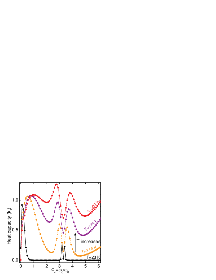
Figure 22: (Color online) The heat capacity vs magnetic field of a three-electron quantum dot with the magnetic ion located at $(0.41l_{0},0)$, $\lambda_{C}=0.2$, at several temperatures: $23$, $116$, $174$ and $209$ K.

Now we examine the behavior of the heat capacity at a specific temperature as function of magnetic field. Figs. 22, 23, and 24 are the plots of the magnetic field dependence of the heat capacity of three (at two Coulomb interaction regimes) and four-electron quantum dots at some specific temperatures and two different $\lambda_{C}=0.2,0.5$. The peak at small magnetic fields broadens and moves to higher fields with increasing temperature. The heat capacity exhibits a number of peaks and a clear minimum around e.g. $\omega_{c}=3.4$ as shown in Figs. 22. Remember that this field corresponds to a cusp in the energy versus magnetic field behavior as discussed previously in subsection III.A. At very low temperatures, this cusp still affects the heat capacity through the sharpness of the minimum as shown in the figure and this gradually becomes small at high temperatures. In Fig. 23, we see a very interesting behavior of the heat capacity at $\Omega_{c}\approx 2.3$: the single peak becomes a double peak as temperature increases from $T=5.8$ to $T=11.6K$. This is due to the cusps now occurring around this field in the low-energy levels of the spectrum of the three-electron quantum dot system as observed in Fig. 18. Besides, the structure of the heat capacity is more complex (more peaks) with increasing $\lambda_{C}$. This is made clear if one looks back to the previous discussion related to Figs. 1 and  2(a).

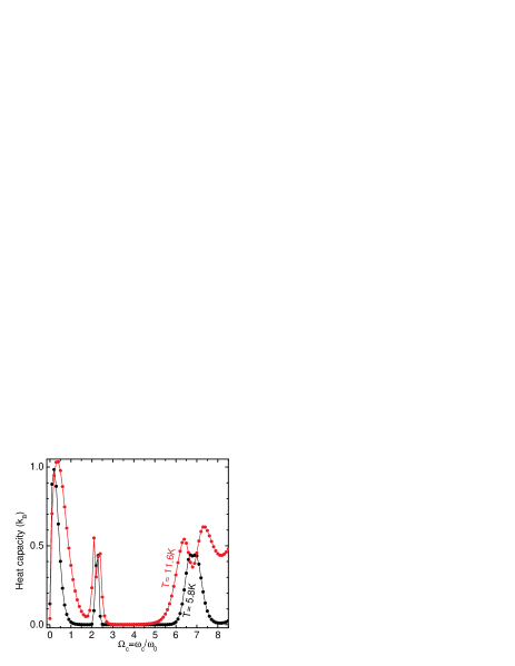
Figure 23: (Color online) The heat capacity vs magnetic field of a three-electron quantum dot with the magnetic ion located at $(0.5l_{0},0)$, $\lambda_{C}=0.5$, and the temperatures are $5.8K$ and $11.6K$.

For the case $N_{e}=4$, the heat capacity exhibits more peaks as compared to the case $N_{e}=3$ and the behavior of the peaks with increasing temperature is also very different. Temperature affects the heat capacity of the system in the sense that it increases the peak values and separates them in magnetic field.

The Coulomb interaction strength changes the structure of the magnetic field dependence of the heat capacity and is illusive through Figs. 22 and 23. The peak of the heat capacity for the case with smaller Coulomb interaction strength appears at higher magnetic field as compared to the case with larger one.

VI Discussions.

Due to the presence of the magnetic ion (and electron-electron interaction), electrons in the ground state do not always completely polarize in the presence of an external magnetic field. The configurations are mixed consisting of electrons having spins up and down. But for very large magnetic field, the magnetic ion tends to pull the electrons closer to the ion forming a ring-like electron density profile. These are the consequences of the interplay of several effects such as the Zeeman effect (on the electrons’ and the magnetic ion’s spins), the Coulomb repulsion, the spin exchange interaction, etc. This competition results in a crossover from ferromagnetic- to antiferromagnetic coupling between the electrons and the magnetic ion at some specific magnetic field. Interestingly, this effect is observed to appear at higher magnetic field when we move the magnetic ion further from the origin of the quantum dot. A re-entrant behavior of the FM-AFM transition is found as function of the Coulomb interaction strength when the magnetic ion is moved out (but not too far) from the center of the quantum dot.

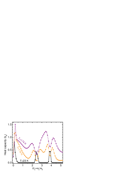
Figure 24: (Color online) The heat capacity vs magnetic field of a four-electron quantum dot with the magnetic ion located at $(0.41l_{0},0)$, $\lambda_{C}=0.2$ plotted for several temperatures.

The energy levels exhibit cusps as function of the magnetic field which correspond to changes of the configuration of the system as expressed by the values of ($<S_{z}>,<L_{z}>$). These cusps move to lower magnetic field with increasing Coulomb interaction strength. The number of cusps increases with increasing number of electrons. These cusps show up in the addition energy.

The transformation of the electron system to those of composite fermions is studied. In high magnetic fields, the electrons attach an even number of quantized vortices which we made clear by examining the many-body ground-state wave function in the presence of a magnetic ion. Unlike the case without a magnetic ion where all the vortices are tightly bound to the electrons, when we fix the electrons at different positions the system of vortices stays pinned to the electrons and moves with the electrons but the relative positions of the vortices are modified.

The contribution of the local Zeeman splitting energy to the total energy of the system in large external fields is very small as compared to the contributions from the other parts. However, a slight movement of the position of the magnetic ion inside the quantum dot affects the result, slightly.

With increasing applied magnetic field, each time the system jumps to a different $(<L_{z}>,<S_{z}>)$ configuration leads to the appearance of a peak in the thermodynamic quantities as e.g. the susceptibility and the heat capacity. In the presence of the magnetic ion, the structure of peaks in the heat capacity changes with the position of the magnetic ion. As temperature increases, these peaks split into two peaks and become smoother.

VII Acknowledgments

This work was supported by FWO-Vl (Flemish Science Foundation), the EU Network of Excellence: SANDiE, and the Belgian Science Policy (IAP).

References

- (1) J. K. Furdyna, J. Appl. Phys. 64, R29 (1988).
- (2) D. L. Klein, R. Roth, A. K. L. Lim, A. P. Alivisatos, and P. L. McEuen, Nature (London) 389, 699 (1997).
- (3) Y. F. Chen, J. H. Huang, W. N. Lee, T. S. Chin, R. T. Huang, F. R. Chen, J. J. Kai, and H. C. Ku, Appl. Phys. Lett. 90, 022505 (2007).
- (4) K. Chang, J. B. Xia, and F. M. Peeters, Appl. Phys. Lett. 82, 2661 (2003).
- (5) A. O. Govorov, Phys. Rev. B 72, 075358 (2005).
- (6) Paul I. Archer, Steven A. Santangelo, and Daniel R. Gamelin, Nano Lett. 7, 1037 (2007).
- (7) J. Fernández-Rossier and L. Brey, Phys. Rev. Lett. 93, 117201 (2004); L. Besombes, Y. Léger, L. Maingault, D. Ferrand, H. Mariette, and J. Cibert, Phys. Rev. Lett. 93, 207403 (2004); Y. Léger, L. Besombes, L. Maingault, D. Ferrand, and H. Mariette, Phys. Rev. Lett. 95, 047403 (2005); Phys. Rev. B 72, 241309(R) (2005); L. Maingault, L. Besombes, Y. Léger, C. Bougerol, and H. Mariette, Appl. Phys. Lett. 89, 193109 (2006).
- (8) T. Schmidt, M. Scheibner, L. Worschech, A. Forchel, T. Slobodskyy, and L. W. Molenkamp, J. Appl. Phys. 100, 123109 (2006).
- (9) P. Wojnar, J. Suffczyński, K. Kowalik, A. Golnik, G. Karczewski, and J. Kossut, Phys. Rev. B 75, 155301 (2007).
- (10) J. Fernández-Rossier and Ramón Aguado, Phys. Rev. Lett. 98, 106805 (2007).
- (11) Y. Léger, L. Besombes, J. Fernández-Rossier, L. Maingault, and H. Mariette, Phys. Rev. Lett. 97, 107401 (2006); L. Maingault, L. Besombes, Y. Léger, H. Mariette, and C. Bougerol, Phys. Stat. Sol. (c) 3, 3992 (2006); M. M. Glazov, E. L. Ivchenko, L. Besombes, Y. Léger, L. Maingault, and H. Mariette, Phys. Rev. B 75 205313 (2007).
- (12) M. B. Tavernier, E. Anisimovas, F. M. Peeters, B. Szafran, J. Adamowski, and S. Bednarek, Phys. Rev. B 68, 205305 (2003); M. B. Tavernier, E. Anisimovas, and F. M. Peeters, Phys. Rev. B 70, 155321 (2004); Phys. Rev. B 74, 125305 (2006); T. Stopa, B. Szafran, M. B. Tavernier, and F. M. Peeters, Phys. Rev. B 73, 075315 (2006).
- (13) Shun-Jen Cheng, Phys. Rev. B 72, 235332 (2005).
- (14) Fanyao Qu and Pawel Hawrylak, Phys. Rev. Lett. 95, 217206 (2005); ibid. 96, 157201 (2006).
- (15) Nga T. T. Nguyen and F. M. Peeters, Phys. Rev. B 76, 045315 (2007).
- (16) Ramin M. Abolfath, Pawel Hawrylak, and Igor Z̆utić, Phys. Rev. Lett. 98, 207203 (2007).
- (17) J. K. Jain, Phys. Rev. Lett. 63, 199 (1989); Phys. Rev. B 41, 7653 (1990); 42, 9193(E)(1990).
- (18) H. Saarikoski, A. Harju, M. J. Puska, and R. M. Nieminen, Phys. Rev. Lett. 93, 116802 (2004).
- (19) S. Tarucha, D. G. Austing, T. Honda, R. J. van der Hage, and L. P. Kouwenhoven, Phys. Rev. Lett. 77, 3613 (1996).