Exploration of Order in Chaos with Replica Exchange Monte Carlo

Abstract

A method for exploring unstable structures generated by nonlinear dynamical systems is introduced. It is based on the sampling of initial conditions and parameters by Replica Exchange Monte Carlo (REM), and efficient both for the search of rare initial conditions and for the combined search of rare initial conditions and parameters. Examples discussed here include the sampling of unstable periodic orbits in chaos and search for the stable manifold of unstable fixed points, as well as construction of the global bifurcation diagram of a map.

1 Introduction

Nonlinear dynamical systems exhibit very complex structures in the phase space [1, 2]. There can be a number of stable or unstable fixed points, periodic orbits, chaotic saddles, and more intricate invariant manifolds. Basin structures corresponding to these invariant manifolds can also be very complicated. Quest for these structures is an important subject in the study of dynamical systems.

It is, however, not easy to capture these global structures by time evolution from randomly chosen initial conditions, because they are often unstable and correspond to very rare initial conditions. Analysis of these structures requires an efficient algorithm for sampling rare trajectories from rare initial conditions, which acts as an anatomical tool of nonlinear dynamical systems. Moreover, properties of chaotic or multi-basin dynamical systems are often sensitive to the choice of values of the parameters. Then, additional complexity arises when we do not have precise knowledge on the values of parameters with which interesting structures appear. Algorithm with which we can perform combined search of the space of initial conditions and of the parameter space is required for analyzing dynamical systems.

In this paper, we introduce a method based on Markov Chain Monte Carlo (MCMC) [3, 4, 5], which is efficient both for the search of rare initial conditions and for the combined search of rare initial conditions and parameters. In the proposed algorithm, we identify initial conditions of trajectories as microscopic states to be sampled, and assign each of them an artificial “energy” that represents a measure of “atypicality” of the trajectory starting from the initial condition. These initial conditions are sampled by MCMC and a set of atypical trajectories is obtained. This approach is easily extended to the combined search of the space of initial conditions and of the parameter space. An essential idea is the use of direct product of initial conditions and parameter as a state space explored by MCMC.

In both cases, however, naive applications of MCMC will be impaired by sensitive dependence on initial conditions and parameters in nonlinear dynamical systems, which lead to a highly multimodal energy function. Here we use Replica Exchange Monte Carlo (REM), which is also known as Parallel Tempering (PT), to circumvent the difficulty. REM is useful for the sampling on a rugged energy surface and intensively used for the finite-temperature simulation of spin glass [6, 7] and biomolecules [8, 7]. When we generate multiple samples with conventional optimization methods, such as simulated annealing, it is difficult to control the probability of repeated appearance of the same (or similar) items in an obtained set of samples. The advantage of REM is that it realizes unbiased sampling from the given ensemble even in the region corresponding to low “temperatures”.

The idea of using MCMC or related algorithm for sampling rare trajectories in nonlinear dynamical systems is already seen in literature [9, 10, 11, 12, 13, 14, 15], while combined search of initial conditions and parameters is rarely studied.

These studies are classified into two categories. Some of them [9, 10, 11, 12, 13], including an earlier work [9] and recent studies [13, 12], developed frameworks where the states to be sampled by the algorithm are entire trajectories or orbits, instead of initial conditions of the trajectories. The “transition path sampling” [16, 10, 11, 17], which mostly used for sampling trajectories between two metastable states, is also based on a similar choice of state space, that is, a state consists of the array of positions (and momentums) of particles at all time-steps in a trajectory. The algorithm proposed in this paper is much simplified with the choice of initial condition as state variable. It is also a natural choice for a deterministic but not necessary reversible dynamical system. In the following sections, we will show that the proposed algorithm can deal with impressively various kinds of problems.

Another type of algorithm proposed in [14, 15] approximates “pseudo trajectories” with desired property by a set of particles each of which obeys original equation of motion. Using a genetic algorithm like split/delete procedure, efficient sampling of rare trajectories is realized. It is a kind of sequential Monte Carlo [18, 19] or diffusion Monte Carlo [20, 19] and not genuine MCMC. It can also be interpreted as a multi-particle version of ingenious “staggered-step” algorithm [21] developed earlier. The idea seems effective for trajectories with positive Lyapunov numbers, but its advantage might be reduced in a search for trajectories with negative Lyapunov numbers where split trajectories does not diverge fast without strong external noise. Anyway, it seems to capture different aspects of chaotic systems and will be complementary to the method proposed in this paper.

The organization of the paper is as follows: In Section.2, we explain the basics of the proposed method. In Section.3, two examples of initial condition sampling are discussed. The first one is a toy example of the sampling of the unstable periodic orbits of the Lorenz model. The second one is sampling of stable manifold of the unstable fixed points of a double pendulum with dissipation, which is a much difficult and interesting example. In Section.4, search of parameter space and combined search of parameter space and initial condition space with a modified algorithm are studied. Section.5 devoted to the discussion on the results and possibility of further extensions.

2 Method

2.1 State Vector

In the basic algorithm for the discrete time dynamics with a given set of parameters, the initial condition $X=(x_{1},...,x_{n})\in\mathbb{R}^{n}$ of a trajectory is used as a state variable that characterizes the trajectory evolving from the initial condition. In a continuous time case, it is often better to include the time $T$ when desired phenomena occur. Then a state will be $X=(x_{1},\ldots,x_{n},T)\in\mathbb{R}^{n+1}$. Finally, when the parameters are also unknown, the state vector will be $X=(x_{1},\ldots,x_{n},T,\alpha_{1},\ldots,\alpha_{m})\in\mathbb{R}^{n+1+m}$, where $\alpha=(\alpha_{1},\ldots,\alpha_{m})$ is a vector of unknown parameters.

2.2 Energy Function and Gibbs Distribution

In order to explore rare structures in phase space, we should construct a fictitious “energy” function $E(X)$ defined on the state space. The function depends on the kind of rare orbit we want to explore. For the detection of periodic orbits of a map $x_{n+1}=f(x_{n})$, a simply possibility of the energy function is $E(x_{0})=\log(|f^{n}(x_{0})-f(x_{0})|)$, where the state $X$ coincides with the initial condition $x_{0}$ of the iteration. The other choices of the energy function to explore atypical structure in phase space are shown in Sec. 4, where $E$ may depend also on $T$ and $\alpha$.

Once we define the energy function, it is straightforward to define the Gibbs distribution with the energy

$$p(X)=\frac{\exp(-\beta E(X))}{Z(\beta)}{},\qquad Z=\int\exp(-\beta E(X))dX{}_{.}$$ (1)

While $p(X)$ coincides with the uniform density in a prescribed region when $\beta$ takes a small value, it concentrate to regions with small values of $E$ when $\beta$ becomes large, where we can collect samples of trajectories (and parameters) of desired properties.

2.3 Metropolis Algorithm

Now, the problem of sampling atypical trajectories is reduced to the sampling from the density $p(X)$. Here we use the Metropolis algorithm [22], a simplest implementation of the idea of MCMC. The Metropolis algorithm used here is essentially the same as the standard one commonly used in statistical physics. There is, however, an important difference in actual implementation, that is, we should simulate the trajectories of the length $T$ from the initial condition $x$ with the parameter $\alpha$ at each trial of changing $x$, $T$, and $\alpha$. If we explicitly represent this difference, the iteration of algorithm is described as follows.

1. Draw a perturbation to current states $(\triangle x,\triangle T,\triangle\alpha)$ from a prescribed “trial” density $q$, which defines a move set. Hereafter, the mirror symmetry

   $$q(-\triangle x,-\triangle T,-\triangle\alpha)=q(\triangle x,\triangle T,\triangle\alpha)$$

   of the density $q$ is assumed. Then, when the current values of $(x,T,\alpha)$ is $(x^{(n)},T^{(n)},\alpha^{(n)})$, the candidate of the next states is defined as $(x^{\prime},T^{\prime},\alpha^{\prime})=(x^{(n)}+\triangle x,T^{(n)}+\triangle T,\alpha^{(n)}+\triangle\alpha)$.

2. Run the simulation of length $T^{\prime}$ of the dynamical system with parameter $\alpha^{\prime}$ from the initial condition $x^{\prime}$. From the result, $E(\alpha^{\prime},T^{\prime},x^{\prime})$ is computed.

3. Draw a uniform random number $R\in[0,1]$. If and only if

   $$R<\frac{\exp(-\beta E(x^{\prime},T^{\prime},\alpha^{\prime}))}{\exp(-\beta E(x^{(n)},T^{(n)},\alpha^{(n)}))}{}\ ,$$

   the new proposal is accepted: $x^{(n+1)}=x^{\prime},\,T^{(n+1)}=T^{\prime},\,\alpha^{(n+1)}=\alpha^{\prime}{}_{.}$ Else nothing is changed: $x^{(n+1)}=x^{(n)},\,T^{(n+1)}=T^{(n)},\,\alpha^{(n+1)}=\alpha^{(n)}$

4. Return to Step (i).

An important point for treating unstable structures in potentially chaotic systems is the choice of the density $q$, or, equivalently, the set of moves. The point is that the moves should be hierarchical for the efficient sampling, that is, the coexistence of tiny and large changes in phase space is essential [21]. Here we adopt the method introduced in [21], that is, the elements $\triangle x_{i}$ of the perturbation $\triangle x$ is given by $\delta x_{i}=s\times d\times 10^{-e}$ where $d$ and $e$ are random integers uniformly distributed in $d\in[1,9]$ and $e\in[N_{e}^{\min},N_{e}^{\max}]$, and $s$ is a binary random number that takes the value $\pm 1$ with probability 0.5, respectively. The parameters $N_{e}^{\min}$ and $N_{e}^{\max}$ of the algorithm define the logarithmic scales of the largest and smallest perturbations. The corresponding trial density $q(x_{i})$ becomes a mixture of uniform distributions with the different scales. It has a sharp peak near zero as well as a very long tail. The components of $\triangle\alpha$ and $\triangle T$ are also generated by a similar way.

This version of Metropolis algorithm appears to provide a simple and universal way of treating the Gibbs distribution (1). The efficiency of the algorithm, however, can be reduced when $\beta$ become large in the case of a highly multimodal energy function. This difficulty will be treated by replica exchange Monte Carlo algorithm described in the next subsection.

2.4 Replica Exchange Monte Carlo

Replica exchange Monte Carlo (REM) provides an efficient way to investigate systems with rugged free-energy landscapes [23, 24, 7], particularly at low temperatures. In the present context, it is used in references [12, 13] for the sampling of unstable orbits. It is also used in the framework of “transition path sampling” in references [11, 17].

In a replica exchange Monte Carlo simulation, a number of systems $\{X_{(m)}\}$ with different inverse temperatures $\beta_{m}$ (replicas) are simulated in parallel. At regular intervals, an attempt is made to exchange the configurations of selected, usually adjacent, pair of replicas. It is accepted with the probability

$$P(X_{(m+1)}\leftrightarrow X_{(m)})=\min[1,\exp(\Delta\beta\Delta E)],$$

where $\Delta\beta=\beta_{m+1}-\beta_{m}$ is the difference between the inverse temperature of the two replicas and $\Delta E=E(X_{(m+1)})-E(X_{(m)})$ is the energy difference of them.

The exchange of replicas with different temperatures effectively reproduces repeated heating and annealing, which avoids trapping in local minima of the energy. Note that it is especially useful with hierarchical moves defined in the previous subsection, because large moves are accepted at high temperatures and tiny moves are dominated at low temperatures.

On the other hand, the above rule of stochastic exchange preserves the joint probability distribution

$$\prod_{m}P_{\beta_{m}}(X_{(m)})$$

as shown in the literature, e.g., [24]. Thus, even with the annealing effect, the probability distribution of each replica $X_{(m)}$ coincides with $P_{\beta_{m}}(X_{(m)})$, which means that an unbiased set of samples is obtained at all inverse temperatures $\{\beta_{m}\}$.

3 Initial Condition Sampling

In this section, we give examples of the initial state sampling by the proposed method. An example is the search for unstable periodic orbits (UPOs) of the Lorenz model. Another interesting example is sampling of rare orbits in a double pendulum system, i.e., initial conditions that locate on the stable manifold of unstable fixed points are sampled by the proposed method.

3.1 Unstable Periodic Orbits of the Lorenz model

In this subsection, we show that unstable periodic orbits (UPOs) in a continuous-time dynamical system can be detected by the proposed method. UPOs are considered as important objects that govern the properties of chaos [2] and there are considerably many works that deal with the computation of UPO [25, 26, 27, 28, 12, 13]. Our purpose here is to show that how the proposed method works with a familiar example, but not to prove that the proposed method is superior to all of these existing methods. It will be, however, useful to note that the proposed method with REM can generate UPOs uniformly under the assumption of uniform measure in the space of initial conditions. This suggests that it can be useful for the global search for UPOs in combination with other methods.

Here, we consider the Lorenz equations [29, 30]

$$\left\{\begin{array}[]{ll}\dot{x}=\sigma(y-z)\\ \dot{y}=rx-y-xz\\ \dot{z}=xy-bz,\end{array}\right.$$ (2)

as a typical continuous-time chaotic system, where $\sigma,r$ and $b$ are parameters of the system. The state of the system is denoted in a vector format as $\vec{x}=(x,y,z)$ and the initial condition is written as $\vec{x}_{0}=(x_{0},y_{0},z_{0})$. The flow generated by the dynamical system (2) is expressed as $\varphi^{t}$, and the orbit determined by the initial condition $\vec{x}_{0}$ is written as $\vec{x}_{t}=\varphi^{t}(\vec{x}_{0})$.

The state sampled by REM is defined by $X\equiv(\vec{x}_{0},T)=(x_{0},y_{0},z_{0},T)$. Then, a candidate of the energy function is given as

$$E(\vec{x}_{0},T)=\log(|\varphi^{T}(\vec{x}_{0})-\vec{x}_{0}|+\epsilon).$$ (3)

The parameter $\epsilon\ll 1$ is a constant for avoiding the divergence of the energy. When the orbit $\{\varphi^{t}(\vec{x}_{0}):t\in\mathbb{R}\}$ is periodic, there exists a time $T$ such that $\varphi^{T}(\vec{x}_{0})=\vec{x}_{0}$, and the energy of the initial condition $\vec{x}_{0}$ takes the minimum value $\log(\epsilon)$.

There are, however, problems with the naive choice (3) of the energy function. First, the energy $E(\vec{x}_{0},0)$ always takes the minimum value, because $\varphi^{0}(\vec{x})=\vec{x}$. Also, when an initial state $\vec{x}_{0}$ locates on a fixed point, the energy of the initial state takes the minimum value for all $T$. This implies that the almost all initial conditions sampled by the above energy function will be in the vicinity of fixed points. To avoid these unfavorable situations, we will add a penalty term $P(\vec{x}_{0},T)$ to the naive energy function (3). An improved energy function is

$$E(\vec{x}_{0},T) = \log(|\varphi^{T}(\vec{x}_{0})-\vec{x}_{0}|+P(\vec{x}_{0},T)+\epsilon)$$ (4)

$$P(\vec{x}_{0},T) = g\left(\frac{1}{T}\int_{0}^{T}{\varphi^{\tau}(\vec{x}_{0})}^{2}d\tau,v_{c}\right)+g(T,T_{c}),$$ (5)

where we use an auxiliary function $g(s,s_{c})=\Theta(s_{c}-s)(\frac{1}{s}-\frac{1}{s_{c}})$. $\Theta(s)$ is the Heviside function defined by $\Theta(s)=1$ if $s\geq 0$ else $\Theta(s)=0$. The first term in the equation (5) represents a penalty for slower “average speed” of the trajectory, where $v_{c}$ is a threshold parameter. When an initial condition is in the vicinity of a stable or unstable fixed point, the orbit stays near the point within a certain time. Then, the averaged speed becomes slower and the value of integral in the penalty term becomes smaller, which causes a large value of the energy. The second term is a penalty to the states that have small $T$, where $T_{c}$ is a threshold parameter.

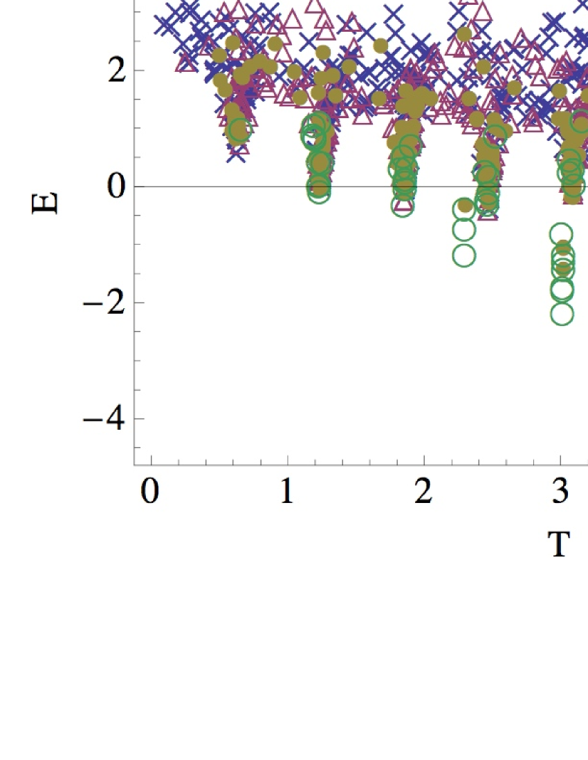
Figure 1: (a) Samples generated by the proposed method are plotted on the $(E,T)$ plane. The crosses, triangles, filled circles, and circles correspond to $\beta=2,3,4,5$, respectively. (b) Samples with the energy lower than $-1.5$ are plotted on the Poincaré section $(x,y,r-1)$. The clusters, each of which corresponds to different minima, are identified by a cluster analysis method and they are plotted by a different symbols. 25 clusters are shown. The inset is a magnification. $\epsilon=10^{-3},N_{e}^{min}=1$, and $N_{e}^{max}=5$.

For sampling of initial condition $\vec{x}_{0}$ of the Lorenz model, we take account of the symmetry $(x,y)\leftrightarrow(-x,-y)$ of the equations. We sample initial conditions from the Poincaré section $\vec{x}_{0}=(x_{0},y_{0},r-1)$, where $x_{0}\in[0,20]$ and $y_{0}\in[0,20]$. The period $T$ of orbits is assumed to be in the interval $[0,6]$. Using the energy function (5), the states $X=(\vec{x}_{0},T)$ are sampled by the proposed method. 31 replicas with $\beta=2.0+0.1i,\ i=0,1,\dots,30$ are used.

The samples obtained by the proposed method are plotted on the $(E,T)$ plane in Fig. 1(a) for different temperatures, which are obtained in parallel in a replica exchange Monte Carlo calculation. For lower temperatures, the energy takes smaller values for specific values of the period $T$, which correspond to UPOs.

In Figure 1(b), the samples of initial conditions with $E(\vec{x}_{0},T)\leq-1.5$ are plotted on the Poincaré section. The initial conditions form clusters and each cluster corresponds to initial condition in the vicinity of a different UPO. In each cluster, we pick up the initial condition that has the minimum energy and calculate orbit $\varphi^{T}(\vec{x}_{0})$ starting from the initial condition. Typical orbits are shown in Fig. 2. These orbits are closed in high precision, i.e., the difference between $\vec{x}_{0}$ and $\varphi^{T}(\vec{x}_{0})$ is in order of $10^{-3}$, indicating that they are UPOs.

By using AUTO software[31], we tested these orbits. An orbit detected by the proposed algorithm is used as an initial guess of a Newton’s method implemented in AUTO. We see that the convergence is remarkably quick, which indicates that the iteration begins “sufficiently near” UPOs. The difference between the output of the Newton’s method and the initial guess is also very small.

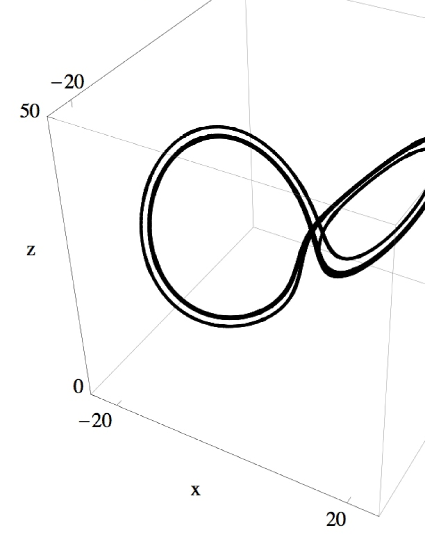
Figure 2: Typical unstable periodic orbits of the Lorenz model sampled by REM are shown. Each orbit is produced from time evolution starting from the initial condition that has the minimum energy in a cluster shown in Fig. 1(b).

3.2 Stable Manifold of Unstable Fixed Points of a Double Pendulum

Let us consider the following dynamics of the double pendulum with dissipation

$$\ddot{\theta_{1}}=\frac{\sin\left(2\left(\theta_{1}-\theta_{2}\right)\right)\dot{\theta_{1}}^{2}+2\sin\left(\theta_{1}-\theta_{2}\right)\dot{\theta_{2}}^{2}+3\sin\left(\theta_{1}\right)+\sin\left(\theta_{1}-2\theta_{2}\right)}{\cos\left(2\left(\theta_{1}-\theta_{2}\right)\right)-3}-k\dot{\theta_{1}},$$

$$\ddot{\theta_{2}}=-\frac{2\sin\left(\theta_{1}-\theta_{2}\right)\left(2\dot{\theta_{1}}^{2}+\cos\left(\theta_{1}-\theta_{2}\right)\dot{\theta_{2}}^{2}+2\cos\left(\theta_{1}\right)\right)}{\cos\left(2\left(\theta_{1}-\theta_{2}\right)\right)-3}-k\dot{\theta_{2}},$$ (6)

where $k$ is a dumping coefficient.

The double pendulum system (3.2) has three unstable fixed points: $(\theta_{1},\dot{\theta_{1}},\theta_{2},\dot{\theta_{2}})=(\pi,0,\pi,0)$, $(\pi,0,0,0)$ and $(0,0,\pi,0)$. Each unstable fixed point corresponds to an “inverted” state of pendulums. Starting from any initial condition $\vec{x}_{0}=(\theta_{1},\dot{\theta_{1}},\theta_{2},\dot{\theta_{2}})=(0,\omega_{1},0,\omega_{2})$, however, almost all trajectories are converged to the stable fixed point $(\theta_{1},\dot{\theta_{1}},\theta_{2},\dot{\theta_{2}})=(0,0,0,0)$ by dissipation originate from the friction at the hinge.

In this system, we try to detect atypical trajectories that converge to unstable fixed points. When an initial condition locates on the stable manifold of an unstable fixed point, the orbit starting from such an initial condition converges to the unstable fixed point after a long time evolution. We search such an atypical initial state on the Poincaré section $(\theta_{1},\dot{\theta_{1}},\theta_{2},\dot{\theta_{2}})=(0,\omega_{1},0,\omega_{2})$.

The state sampled by the proposed method is set as $X=(\omega_{1},\omega_{2},T)$. There are many possibility of the energy function. Here we try to find trajectories converging one of the three fixed points and choose the energy as

$$E(\omega_{1},\omega_{2},T) = \log(E_{k}(\omega_{1},\omega_{2},T)+E_{p}(\omega_{1},\omega_{2},T)),$$

$$E_{k}(\omega_{1},\omega_{2},T) = |\dot{\theta}_{1}(T)|+|\dot{\theta}_{2}^{2}(T)|,$$

$$E_{p}(\omega_{1},\omega_{2},T) = \min[\,\,\cos(\theta_{1}(T))\cos(\theta_{2}(T)),\,\,\cos(\theta_{1}(T))+\cos(\theta_{2}(T))\,\,]+1,$$ (7)

where $E_{k}$ represents “kinetic energy” of the pendulum at time $T$ stating from an initial condition defined by $(\omega_{1},\omega_{2})$. The term $E_{p}$ represents an artificial “potential energy”, which has minimum at each of the three unstable fixed points. Note that if we want to find trajectories converging to a given unstable fixed point, we can use other artificial potential energies such as $E_{p}(\omega_{0},\omega_{1},T)=|\theta_{1}(T)-\pi|+|\theta_{2}(T)-\pi|$. The energy landscape defined by (7) is shown in Fig. 3(a), where the energy $E(\omega_{1},\omega_{2},T)$ vs. $\omega_{1}$ and $\omega_{2}$ is plotted for a fixed time, $T=5$. Rugged structure is clearly seen and increase of the sampling efficiency by REM is expected.

We discuss the result of a simulation with 31 replicas with $\beta_{i}=2.0+0.2i$ for $i=0,1,\dots,30$. In Fig. 3(b), initial states sampled by the proposed method is plotted on the $(\omega_{1},E)$ plane for replicas with inverse temperatures $\beta=0.1,1.1,2.1,3.1,4.1,5.1$. The points are scattered at higher temperatures, but they are concentrated in separated regions when the temperature becomes lower.

Because states with lower energies correspond to desired atypical trajectories, we select a set of the states whose energies $E$ are lower than a threshold $E_{cr}=-5$. We show these states in Fig. 4(a). By using cluster analysis, we divide these initial states into clusters. Since these clusters are well separated in the plane, we identify each cluster as a representation of a qualitatively different set of trajectories.

In each cluster, we identify an initial state that has minimum energy. Figure 4(b) demonstrates atypical trajectories starting from these initial conditions on $(\dot{\theta}_{1},\dot{\theta}_{2})$ plane. It is seen that each cluster corresponds to qualitatively different pattern of motion. Examples of sequences of snapshots for pattern of the double pendulum are shown in Fig. 4(c), each of which corresponds to a trajectory obtained by the above procedure.

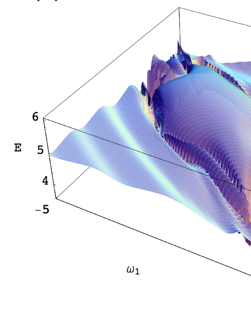
Figure 3: (a) Rugged energy landscape $E(\vec{x}_{0},T)$ with fixed $T=5.0$ as a function of $\omega_{1}$ and $\omega_{2}$. (b) Samples are plotted on $(E,\omega_{1})$ for different temperatures; $\beta=0.1,1.1,2.1,3.1,4.1,5.1$. The sampling is performed by 51 replicas with $\beta=0.1i$ for $i=1,2,\dots,51$. $\epsilon=10^{-5},N_{e}^{min}=1$, and $N_{e}^{max}=9$.

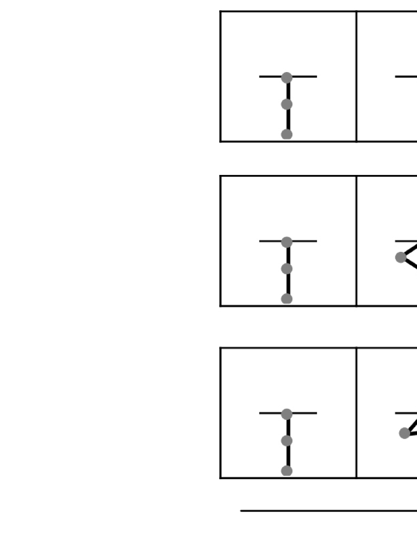
Figure 4: (a) States with $E<-5$ is plotted on the $(\omega_{1},\omega_{2})$ plane. The states form clusters, which are regarded as sets of qualitatively different trajectories. The different cluster is plotted with different symbols in the figure. (b) Typical trajectories starting from the state that has minimum energy within a cluster are plotted on the $(\dot{\theta}_{1},\dot{\theta}_{2})$ plane. Six trajectories are shown. (c) Sequences of snapshots of pattern of the double pendulum that correspond to trajectories. Three trajectories, each of which converges to a different fixed point are shown in the upper, middle, and lower panel. The other parameters are the same as those in Fig. 3

4 Parameter Search and Combined Search

In this section, search in a parameter space and combined search in parameter and initial condition spaces are discussed as an extension of our method. Examples are sampling of the boundary of the Mandelbrot set and exploration of the global bifurcation structure of the logistic map.

4.1 The Boundary of the Mandelbrot Set

For a map $f_{c}(z)=z^{2}+c$ parameterized by a parameter $c\in\mathbb{C}$, consider the sequence $(0,f_{c}(0),f_{c}(f_{c}(0)),\dots)$. The Mandelbrot set [32] is defined as the set of points $c\in\mathbb{C}$ such that the above sequence does not escape to the infinity. Hereafter, we denote $f_{c}(f_{c}(0))=f^{2}_{c}(0))$ and $f_{c}(f_{c}(f_{c}(0)))=f^{3}_{c}(0)$, and so on.

The Mandelbrot set is seen to have an elaborate boundary in the complex plane, which does not simplify at any magnification. This qualifies the boundary as a fractal. In order to compute the boundary of the set, we use the parameter $c$ as a state of the proposed method and employ the following energy function

$$E(c)=-\log(n(c)),$$

where the function $n(c)$ is defined as the smallest $n$ that $|f_{c}^{n}(0)|>2$. If $n>N$ for a prescribed large number $N=200$, we set $n(c)=1$ and $E(c)=0$. In that case, the point $c$ is considered as inside the Mandelbrot set and not on the boundary.

Using this energy function, the boundary of the Mandelbrot set is calculated by the proposed method and the results are shown in Fig. 5. While the points are almost randomly distributed in the complex plane for the replicas with a high temperature $1/\beta$, the distribution of points corresponding to replicas with lower temperature is concentrated on the boundary of Mandelbrot set.

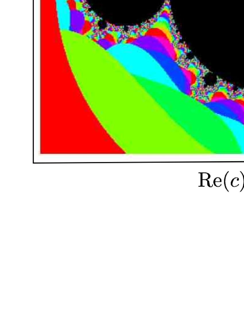
Figure 5: (a) The Mandelbrot set. The black region shows the Mandelbrot set and the outside of the set is colored according to the escape time. (b) The boundary of the Mandelbrot set. Six replicas with $\beta=1.0,2.0,3.0,4.0,5.0,$ and $6.0$ are used for sampling. $N_{e}^{min}=1$ and $N_{e}^{max}=9$.

4.2 Periodic Orbits and Bifurcation Diagram of the Logistic Map

The logistic map [33, 1] is defined by

$$f_{a}(x)=ax(1-x),$$ (8)

where $a\in[0,4]$ is a parameter. Let us consider the energy function

$$E(a,x_{0})=\log(|f_{a}^{k}(x_{0})-x_{0}|+\epsilon),$$ (9)

where $k$ is a given period and $\epsilon$ is a constant that determines the minimum energy. Indeed, we can find initial conditions $x_{0}$ corresponding to period $k$ orbits for a given parameter $a$ using the energy function (9) by the proposed method (the results are not shown here). On the other hand, the extension of sampling state space from $x_{0}$ to $(a,x_{0})$ enables us the study of global bifurcation structure of the periodic solutions. The extension is straightforward, i.e., we sample the vector $(a,x_{0})$ from the Gibbs distribution determined by the same energy function (9) using REM.

In Fig. 6, the result for the period $k=3$ is shown, where sampled points are plotted on the $(a,x_{0})$ plane. We sample orbits from $a\in[3.8,4]$ and $x\in[0,1]$. The points are scattered broadly in the vicinity of the true bifurcation branch of the period $k=3$ orbits at higher temperatures. The dispersion of the points becomes smaller at lower temperatures and periodic orbits with $k=3$ are detected.

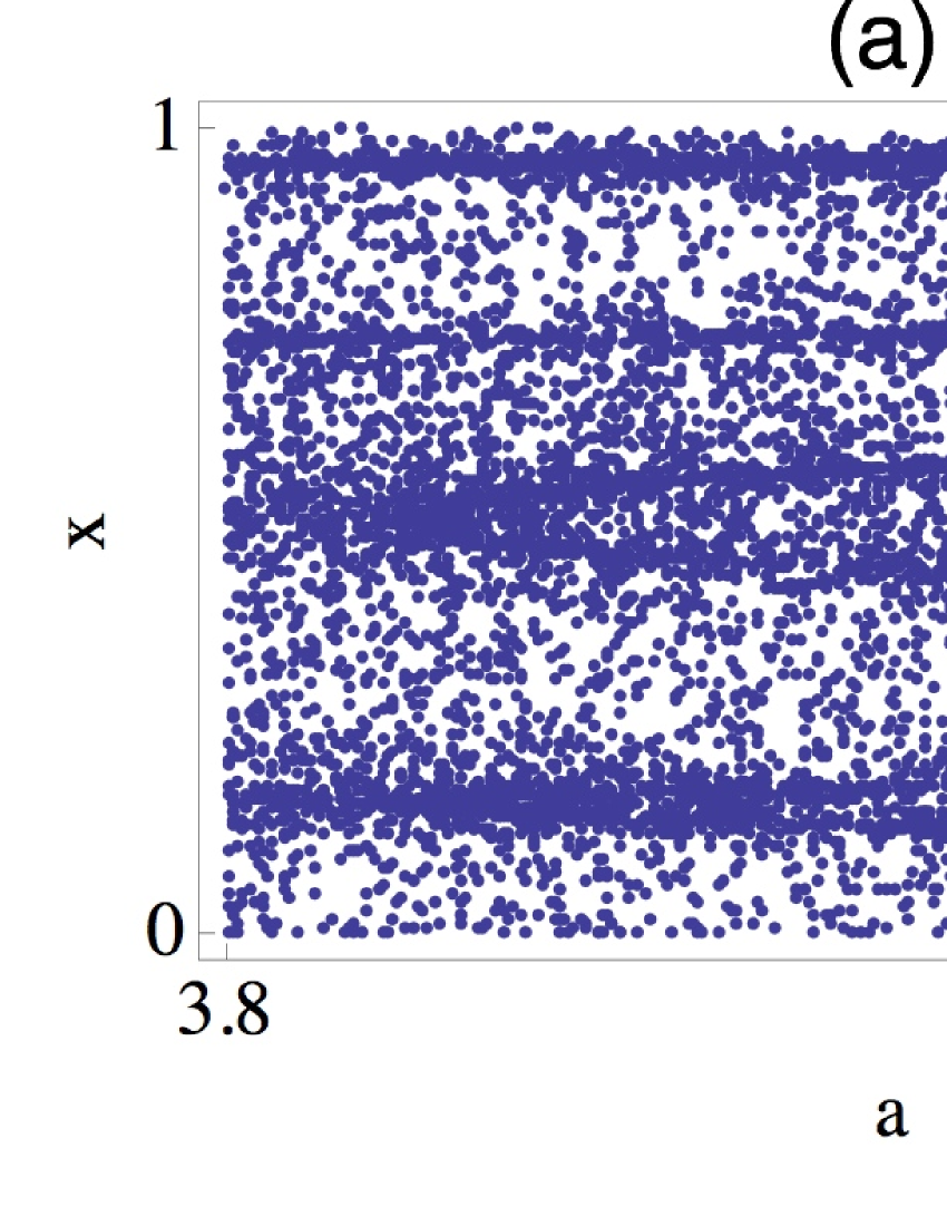
Figure 6: The bifurcation structure of the period three solutions of the logistic map is obtained by the proposed method. Ten replicas are used with $\beta=0.5i$ for $i=1,2,\dots,10$. $\epsilon=10^{-4},N_{e}^{min}=1$, and $N_{e}^{max}=11$. (a) $\beta=0.5$. (b) $\beta=1.0$.

5 Summary and Discussion

In this paper, we presented a general strategy for exploring unstable structures generated by nonlinear dynamical systems. An artificial “energy” is defined as a function of the initial condition of the trajectory and the Gibbs distribution induced by the energy is sampled by the Metropolis method. When an “energy” suitable for the purpose is chosen, sampling from the Gibbs distribution at low temperatures realizes efficient sampling of rare initial conditions that leads to interesting trajectories. Replica exchange Monte Carlo (REM) is used so as to avoid capturing in local minima of the energy landscape.

While implementation of the proposed method is simpler than the methods in which artificial energy is defined in the space of entire trajectories, the method can treat a variety of problem, including the search for unstable periodic orbits of the Lorenz model and stable manifold of unstable fixed points of a double pendulum.

It is also shown that search in the parameter space and combined search of initial conditions and parameters become possible by adding the parameters to the state vector. Two examples shown here are the Mandelbrot set of a complex dynamical system and the bifurcation diagram of the logistic map.

An important future problem is to calculate quantitative results by the proposed method. Examples are the relative densities of initial conditions that lead to different Lyapunov numbers and densities of escape time from a chaotic saddle. These calculations are possible because REM is not only an optimization method, but also realize correct sampling from the Gibbs distribution. It is also interesting to introduce other types of extended ensemble Monte Carlo, such as multicanonical algorithm, for this purpose. Research in this direction is now in progress and the results will be published elsewhere.

The combined search of initial conditions and parameters by the proposed method is also promising and should be tested in the study of more complicated systems. There is, however, an inherent interpretation problem, i.e., the joint density in the direct product of parameter space and initial condition space seems not to have a definite interpretation. The method is already useful to give a rough sketch of the bifurcation diagram, but it will be better if we can give a physical meaning to the joint density.

References

References

- [1] E. Ott. Chaos in Dynamical Systems. Cambridge University Press, 2002.
- [2] P. Cvitanović, R. Artuso, R. Mainieri, G. Tanner, G. Vattay, N. Whelan, and A. Wirzba. Chaos – Classical and Quantum. http://chaosbook.org/, unpublished (web book),.
- [3] D. Landau and K. Binder. A Guide to Monte Carlo Simulations in Statistical Physics. Cambridge University Press, 2005.
- [4] M. E. J. Newman and G. T. Barkema. Monte Carlo Methods in Statistical Physics. Oxford University Press, 1999.
- [5] J. Liu. Monte Carlo Strategies in Scientific Computing. Springer, 2001.
- [6] A. P. Young, editor. Spin Glasses and Random Fields. World Scientific, 1997.
- [7] W. Janke, editor. Rugged Free Energy Landscapes: Common Computational Approaches to Spin Glasses, Structural Glasses and Biological Macromolecules. Lect. Notes Phys. Vol. 736. Springer, Berlin, 2008.
- [8] A. Mitsutake, Y. Sugita, and Y. Okamoto. Generalized-ensemble algorithms for molecular simulations of biopolymers. Biopolymers (Peptide Science), 60:96–123, 2001.
- [9] D. L. Freeman A. E. Cho, J. D. Doll. The construction of double-ended classical trajectories. Chemical Physics Letters, 229:218–224, 1994.
- [10] Peter G. Bolhuis, Christoph Dellago, and David Chandler. Sampling ensembles of deterministic transition pathways. Faraday Discuss., 110:421–436, 1998.
- [11] T.J.H. Vlugt and B. Smit. On the efficient sampling of pathways in the transition path ensemble. Phys. Chem. Comm., 2:Art. No. 2, 2000.
- [12] M. Kawasaki and S.I. Sasa. Statistics of unstable periodic orbits of a chaotic dynamical system with a large number of degrees of freedom. Phys. Rev. E, 72:037202, 2005.
- [13] S.I. Sasa and K. Hayashi. Computation of the Kolmogorov-Sinai entropy using statistitical mechanics: Application of an exchange Monte Carlo method. Europhys. Lett., 76:156–162, 2006.
- [14] C. Giardiná, J. Kurchan, and L. Peliti. Direct evaluation of large-deviation functions. Phys. Rev. Lett., 96:120603, 2006.
- [15] Julien Tailleur and Jorge Kurchan. Probing rare physical trajectories with Lyapunov weighted dynamics. Nature Physics 3, 3:203–207, 2007.
- [16] P. G. Bolhuis, D. Chandler, C. Dellago, and P. Geissler. Transition path sampling: Throwing ropes over mountain passes, in the dark. Ann. Rev. of Phys. Chem., 59:291–318, 2002.
- [17] T. S. van Erp. Reaction rate calculation by parallel path swapping. Phys. Rev. Lett., 98:268301, 2007.
- [18] A. Doucet, N. De Freitas, and N. Gordon, editors. Sequential Monte Carlo Methods in Practice. Springer, 2001.
- [19] Y. Iba. Population Monte Carlo algorithms. Transactions of the Japanese Society for Artificial Intelligence, 16:279–286, 2001.
- [20] M. H. Kalos. Monte Carlo calculations of the ground state of three- and four-body nuclei. Phys. Rev., 128:1791 – 1795, 1962.
- [21] D. Sweet, H. E. Nusse, and J. A. Yorke. Stagger-and-step method: Detecting and computing chaotic saddles in higher dimensions. Phys. Rev. Lett., 86:2261–2264, 2001.
- [22] N. Metropolis, A.W. Rosenbluth, M.N. Rosenbluth, A.H. Teller, and E. Teller. Equations of state calculations by fast computing machines. J. Chem. Phys., 21:1087–1091, 1953.
- [23] K. Hukushima and K. Nemoto. Exchange Monte Carlo method and application to spin glass simulations. J. Phys. Soc. Jpn., 65:1604–1611, 1996.
- [24] Y. Iba. Extended ensemble Monte Carlo. Int. J. Mod. Phys. C, 12:623–656, 2001.
- [25] O. Biham and W. Wenzel. Characterization of unstable periodic orbits in chaotic attractors and repellers. Phys. Rev. Lett., 63:819 – 822, 1989.
- [26] F. K. Diakonos, P. Schmelcher, and O. Biham. Systematic computation of the least unstable periodic orbits in chaotic attractors. Phys. Rev. Lett., 81:4349 – 4352, 1998.
- [27] R. L. Davidchack and Y.-C. Lai. Efficient algorithm for detecting unstable periodic orbits in chaotic systems. Phys. Rev. E, 60:6172 – 6175, 1999.
- [28] Y. Lan and P. Cvitanović. Variational method for finding periodic orbits in a general flow. Phys. Rev. E, 69:016217, 2004.
- [29] E.N.Lorenz. Deterministic non-periodic flow. J. Atm. Sci., 20:130–140, 1963.
- [30] C. Sparrow. The Lorenz Equations: Bifurcations, Chaos, and Strange Attractors. Springer-Verlag, New York, 1982.
- [31] E. J. Doedel, R. C. Paffenroth, A. R. Champneys, T. F. Fairgrieve, Yu. A. Kuznetsov, B. Sandstede, and X. Wang. Auto 2000: Continuation and bifurcation software for ordinary differential equations (with homcont). Technical Report, Caltech, 2001.
- [32] B. B. Mandelbrot. Fractals and Chaos: The Mandelbrot Set and Beyond. Springer, 2004.
- [33] R.May. Biological populations with nonoverlapping generations: Stable points,stable cycles,and chaos. Science, 186:645, 1974.