Quantifying evolvability in small biological networks

Abstract

We introduce a quantitative measure of the capacity of a small biological network to evolve. We apply our measure to a stochastic description of the experimental setup of Guet et al. (Science 296:1466, 2002), treating chemical inducers as functional inputs to biochemical networks and the expression of a reporter gene as the functional output. We take an information-theoretic approach, allowing the system to set parameters that optimize signal processing ability, thus enumerating each network’s highest-fidelity functions. We find that all networks studied are highly evolvable by our measure, meaning that change in function has little dependence on change in parameters. Moreover, we find that each network’s functions are connected by paths in the parameter space along which information is not significantly lowered, meaning a network may continuously change its functionality without losing it along the way. This property further underscores the evolvability of the networks.

Many signals in cells are processed using a network of interacting genes: exogenous signals affect expression of genes coding for transcription factor proteins, which in turn regulate the expression of other genes. Although early works have suggested that the connectivity of such regulatory networks dictates their function Shen-Orr et al. (2002); Mangan and Alon (2003); Kollmann et al. (2005), recent studies offer evidence that a network with fixed connectivity can change its function simply by varying its biochemical parameters Wall et al. (2005); Ziv et al. (2007); Voigt et al. (2005); Guet et al. (2002). The diversity of a network’s achievable functions and the ease with which it can realize them are central to its capacity to evolve epigenetically, without slow and costly modifications to the genetic code, and thus central to the evolutionary capacity of the organism as a whole.

The evolvability of a regulatory network has been a topic of much discussion in recent literature Voigt et al. (2005); Ptashne and Gann (1998); Kitano (2004); Buchler et al. (2003); Braunewell and Bornholdt (2008); Kashtan and Alon (2005), but little has been done to quantify the concept in a principled way. Here we propose a quantitative measure of network evolvability, and we apply it to a set of small regulatory networks, such that a principled comparison can be made across networks. Networks are taken from the experimental setup of Guet et al. Guet et al. (2002) and modeled stochastically. We find biochemical parameters that optimize the information flow between a chemical “input” signal and a particular “output” gene, and we indeed find that a single network performs different functions at different sets of optimal parameters. We argue that a more evolvable network will be able to access a richer diversity of its functions with smaller changes in its parameters, and as such we quantify evolvability using a measure of anti-correlation between parametric and functional change.

We find that while there are small differences among networks’ evolvability scores, all are highly evolvable, meaning that the magnitude of a functional change has little dependence on the parametric change required to produce it. Moreover, we find that transitions among a network’s optimally informative functions can be made without significant loss of the input-output information along the way. By proposing and demonstrating a principled evolvability measure, we reveal these features quantitatively; both features suggest a high capacity of the studied regulatory networks to evolve.

I Methods

First we briefly outline the methods used to develop a quantitative measure of evolvability; each step is discussed in more detail in the sections that follow. The system of interest is a small (4-gene) transcriptional regulatory network. As in Guet et al. Guet et al. (2002), we treat the presence or absence of chemical inducers (small molecules that affect the efficacy of the transcription factors) as the inputs to the network, and the expression of a particular gene as the output. We use a stochastic model to find expression level distributions at a steady-state, and we search for the model parameters which maximize the mutual information between input and output. We characterize the function that the network performs by the order in which the output distributions corresponding to each input state are encoded Mugler et al. (2008); a single network can perform different functions at different parameter settings. We define the evolvability of the network as the ability to perform a diverse set of functions with only small changes in parameters, and we quantify evolvability accordingly using a measure of anti-correlation between pair-wise function distance and parameter distance.

I.1 Model

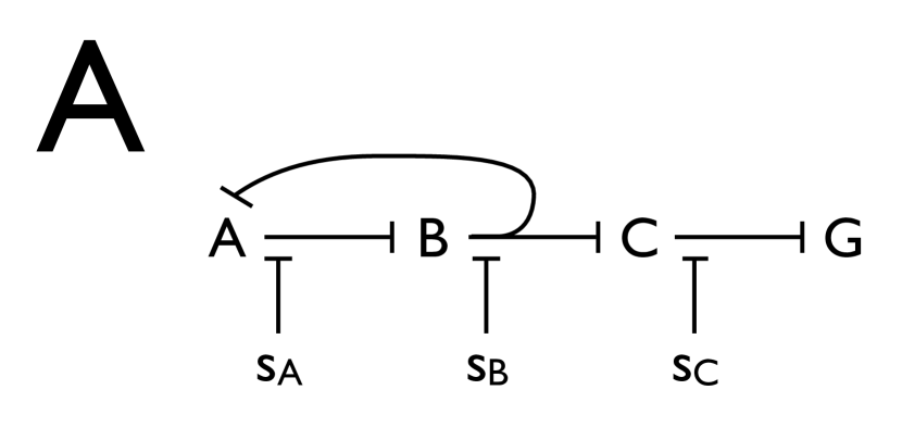
Following the experimental setup of Guet et al. Guet et al. (2002), we study all networks that can be built out of three genes $A$, $B$, and $C$, in which each gene is regulated by one other gene, and regulation edges can be up-regulating or down-regulating. Additionally, as in the experiment, gene $C$ down-regulates a “reporter” gene $G$ (e.g., GFP), whose expression we treat as the functional output of the network. This yields a total of 24 networks, as shown on the horizontal axis of Figure 2. Also in analogy to the experiment, the efficacy of each transcription factor can be inhibited by the presence of a chemical inducer $s$, a small molecule that binds to the transcription factor and lowers its affinity for its binding site. The presence or absence of the chemical inducers $s_{A}$, $s_{B}$, and $s_{C}$ corresponding to each transcription factor $A$, $B$, and $C$ define the functional input state of the network. The inhibitory effect of each inducer is illustrated for an example network in the top panel of Figure 1A, and the eight possible input states $i$, determined by the presence or absence of the inducers, are listed in the bottom panel.

For a typical regulatory network inside a cell, intrinsic noise arising from fluctuations in the small numbers of species Elowitz et al. (2002); Thattai and van Oudenaarden (2001) is the primary factor limiting transmission of information from a chemical input to a genetic output Ziv et al. (2007); Acar et al. (2005); Pedraza and Oudenaarden (2005); Mugler et al. (2008). This observation has two important consequences for modeling: (a) a realistic model should capture not just mean protein concentrations, but probability distributions over numbers of proteins Shahrezaei and Swain (2008); Hornos et al. (2005), and (b) the most biologically relevant model parameters will retain an optimal flow of information in the presence of this noise Ziv et al. (2007); Tkacik et al. (2008); Doan et al. (2006).

The first consequence is most fully addressed by solving the chemical master equation van Kampen (1992), which describes the time-evolution of the joint probability distribution for the numbers of all molecules in the system given the elementary reactions (which are ultimately a function of the network topology). For our systems, the master equation is not analytically solvable. Progress can be made either by Monte-Carlo simulation of the master equation Gillespie (1977), or by approximating the master equation, e.g. with the linear-noise approximation (LNA) Paulsson (2004); Elf and Ehrenberg (2003); van Kampen (1992); Ziv et al. (2007); Mugler et al. (2008). Since it does not rely on sampling, the LNA is much more computationally efficient (and thus more amenable to a search for high-fidelity model parameters), and in previous work Ziv et al. (2007) we found the distributions obtained via the LNA were practically indistinguishable from those obtained via stochastic simulation for copy numbers above $10-20$.

In the LNA, the reaction rates in the master equation are linearized, and the steady-state solution is a multidimensional Gaussian distribution van Kampen (1992); Ziv et al. (2007); Mugler et al. (2008). The individual species’ marginal distributions are thus described at the level of Gaussian fluctuations, with means given by the steady-state solution to the deterministic dynamical system describing mean protein numbers. Mean expression has been modeled with remarkable success by combining transcription and translation into one step Elowitz and Leibler (2000); Gardner et al. (2000); Hasty et al. (2001), and accordingly, for each of our networks, we use the following dynamical system in which species are directly coupled to one another,

$$\frac{dX_{j}}{dt}=\alpha_{j}(X_{\pi_{j}}/s_{\pi_{j}})-R_{j}X_{j},$$ (1)

where the $X_{j}\in\{A,B,C,G\}$ are the expression levels (in units of proteins per cell) of the four genes, the $R_{j}$ are degradation rates, and the $\alpha_{j}$ are production rates which depend on the expression level $X_{\pi_{j}}$ and a scale factor $s_{\pi_{j}}$ of the parent $\pi_{j}$ of gene $j$ (where the parent-children connectivity is determined by the network topology). The scale factors, $s_{\pi_{j}}\in\{s_{A},s_{B},s_{C}\}\geq 1$, incorporate the inhibitory effect of each chemical inducer (when present) by reducing the effective transcription factor concentration; when an inducer is absent, its scale factor is set to 1. Regulation is modeled using Hill functions,

$$\alpha_{j}(x)=\begin{cases}a_{0}+a_{j}\frac{x^{n}}{x^{n}+(K_{j})^{n}}&{\rm up-regulating},\\ a_{0}+a_{j}\frac{(K_{j})^{n}}{x^{n}+(K_{j})^{n}}&{\rm down-regulating},\end{cases}$$ (2)

where $a_{0}$ (kept the same for all genes) is the basal production rate, $a_{0}+a_{j}$ is the maximal production rate, $K_{j}$ is the binding constant or the protein number at which production is half-maximal, and $n$ is the cooperativity, which we set to 2. Note from Eqns. (1-2) that increasing the scale factor can be equivalently interpreted as increasing the effective binding constant or lowering the binding affinity. Steady states of Eqn. (1) are found by solving (using MATLAB’s roots) the polynomial equations that result from setting the left-hand side to zero, and keeping only those solutions for which the Jacobian matrix $J$ of Eqn. (1) has eigenvalues whose real parts are all negative.

The variances of the marginal distributions are the diagonal entries in the covariance matrix $\Xi$, which under the LNA satisfies a Lyapunov equation,

$$J\Xi+\Xi J^{T}+D=0,$$ (3)

where $D$ is a diagonal matrix with, for the system in Eqn. (1), the $j$th entry equal to $\alpha_{j}(X_{\pi_{j}}/s_{\pi_{j}})+R_{j}X_{j}$. Eqn. (3) is solved using a standard Lyapunov solver (MATLAB’s lyap). Since the steady-state distributions are Gaussian under the LNA, the solution is fully specified by the means and the variances. The distributions of particular functional importance are $P(G|i)$, the probability of expressing $G$ reporter proteins per cell given that the chemical inducers are in state $i$.

To address the second consequence, that biologically relevant solutions often optimize information flow in the presence of intrinsic noise Tkacik et al. (2008); Doan et al. (2006), as in previous work Ziv et al. (2007) we allow the system to set parameters that maximize the mutual information $I$ Shannon (1949) between input state $i$ and output expression $G$, where

$$I = \sum_{i}\int dG\,P(i,G)\log_{2}\frac{P(i,G)}{P(i)P(G)}$$ (4)

$$= \frac{1}{|i|}\sum_{i=1}^{|i|}\int dG\,p(G|i)\log_{2}\frac{|i|P(G|i)}{\sum_{i^{\prime}=1}^{|i|}P(G|i^{\prime})}.$$ (5)

Here $I$ is measured in bits, and the second step uses $P(i,G)=P(G|i)P(i)$, $P(G)=\sum_{i^{\prime}}P(i^{\prime},G)$, and an assertion that each input state occurs with equal likelihood (i.e., $P(i)=1/|i|$, where $|i|=8$ is the number of input states) to write $I$ entirely in terms of the model solutions $P(G|i)$.

Two computationally trivial ways for the system to maximize $I$ are (a) to use an unbounded number of reporter proteins $G$ to encode the signal, and (b) to set degradation rates such that $G$ responds on a timescale much longer than that of the upstream genes (called a “stiff” system), which has the effect of averaging out the upstream noise. In contrast, in cells, protein production requires energy, which sets a limit on the number of proteins that a cell can produce, and most protein degradation rates are comparable. Therefore we seek model parameters $\vec{\theta}^{*}$ that optimize a constrained objective function,

$$\vec{\theta}^{*}={\rm argmax}_{\vec{\theta}}\left[I-\lambda\langle{X_{j}}\rangle-\gamma\langle{R_{\pi_{j}}}\rangle/R_{G}\right],$$ (6)

where the constants $\lambda$ and $\gamma$ are a metabolic cost and a constraint against stiffness, respectively, the average $\langle{X_{j}}\rangle$ is taken over all genes, and the average $\langle{R_{\pi_{j}}}\rangle$ is taken over upstream genes $A$, $B$, and $C$. Optimization is performed using a simplex algorithm (MATLAB’s fminsearch) in a $15$-dimensional parameter space, as

$$\vec{\theta} = \{a_{0},a_{A},a_{B},a_{C},a_{G},K_{A},K_{B},K_{C},K_{G},$$ (7)

$$R_{A},R_{B},R_{C},s_{A},s_{B},s_{C}\}$$

($R_{G}$ was fixed at $4\times 10^{-4}s^{-1}$ to set a biologically realistic degradation rate scale).

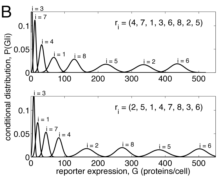
Varying initial parameters yields many local optima $\vec{\theta}^{*}$ at which the input signal may be encoded differently in the output distributions $P(G|i)$. For example, two optimally informative solutions are shown in Figure 1B for the network in Figure 1A. Intuitively, maximizing mutual information has resulted in sets of distributions that are well separated, such that knowledge of the output $G$ would leave little ambiguity about the original input state $i$. We point out, however, that the ordering of the output distributions is different between the two solutions, meaning that the network is performing two different functions at two different points in parameter space. The relationship between diversity of such functions and exploration of parameters is crucial to the discussion of evolvability; in the next section we develop a quantitative measure of evolvability in the context of this system.

I.2 Quantifying evolvability

As seen in several experimental and numerical studies Wall et al. (2005); Ziv et al. (2007); Voigt et al. (2005); Guet et al. (2002), and in data from the model described above, a single regulatory network can perform different functions simply by varying its biochemical parameters. Intuitively, a network should be deemed more evolvable if it is able to access a richer diversity of its functions with smaller changes in its parameters. Quantification of this concept requires definitions of both parametric and functional change.

As in Barkai et al. Barkai and Leibler (1997), we characterize the magnitude of the parametric change in going from one model solution to another by calculating fold-changes in the model parameters. Specifically, we define a parameter distance $\Delta\theta$ between two solutions as the Euclidean distance in the logs of the parameters,

$$\Delta\theta=|\log_{2}\vec{\theta}^{*}_{1}-\log_{2}\vec{\theta}^{*}_{2}|=\sqrt{\sum_{k=1}^{|k|}\left[\log_{2}(\theta^{*}_{1,k}/\theta^{*}_{2,k})\right]^{2}},$$ (8)

where $|k|=15$ is the number of parameters. Under this definition, equal fold-changes in each parameter constitute equal contributions to $\Delta\theta$ (for scale, the doubling of one parameter corresponds to $\Delta\theta=1$).

As in previous work Mugler et al. (2008) and in the original experiment of Guet et al. Guet et al. (2002), we define the function of a network analogously to logic in electrical circuits (AND, OR, XOR, etc.), in which the function is determined by the magnitude of the output’s response to each input state (for example, with two inputs, AND would be defined by a “high” output in response to the $[++]$ state, and a “low” output in response to the $[--]$, $[-+]$, and $[+-]$ states). Since, in our setup, optimizing information produces well-separated output distributions $P(G|i)$ (see Figure 1B), we extend this idea beyond a simple “high” or “low” output classification, and characterize function by the order of the $P(G|i)$. Specifically, we record a vector $\vec{r}$ of ranks of the $P(G|i)$; for example, in the top panel of Figure 1B, the first output distribution ($i=1$) is ranked $4$th, the second ($i=2$) is ranked $7$th, the third ($i=3$) is ranked $1$st, and so on, so the rank vector is $\vec{r}=(4,7,1,\dots)$. We then define the function distance $\Delta f$ between two solutions in terms of the vector distance between their rank vectors,

$$\Delta f=\frac{1}{2}|\vec{r}_{1}-\vec{r}_{2}|^{2}=\frac{1}{2}\sum_{i=1}^{|i|}(r_{1,i}-r_{2,i})^{2}$$ (9)

(for scale, the swapping of two adjacent output distributions corresponds to $\Delta f=1$) . Other function distances, including other permutation distances between the rank vectors, and a continuous distance measure defined by averaging the Jensen-Shannon divergence Lin (1991) between corresponding output distributions in the solution pair, produced similar results, as discussed in the Results section.

It is now clear that, if a network is better able to explore its function set with smaller changes in its parameters (i.e., is more evolvable by our definition), then it will exhibit less correlation between $\Delta f$ and $\Delta\theta$ than other networks. Therefore we define an evolvability score $E$ for a given network as a measure of anti-correlation between $\Delta f$ and $\Delta\theta$, calculated for every pair of its optimal model solutions . Specifically,

$$E=1-(\tau+1)/2,$$ (10)

where $\tau$ is Kendall’s tau Kendall (1938), a nonparametric measure of correlation between all pairwise $\Delta f$ and $\Delta\theta$; we rescale $\tau$ such that $0<E<1$ and take its complement to obtain an anti-correlation. Using a nonparametric correlation statistic has the advantage that our evolvability measure remains invariant upon any monotonic rescaling in the definitions of either $\Delta\theta$ or $\Delta f$. Additionally, we note that $E$ can be thought of as the probability that a pair of solutions drawn at random have a larger $\Delta f$ than another pair given that the first pair had a smaller $\Delta\theta$, or as the fraction of discordant pairs of $(\Delta\theta,\Delta f)$ data points .

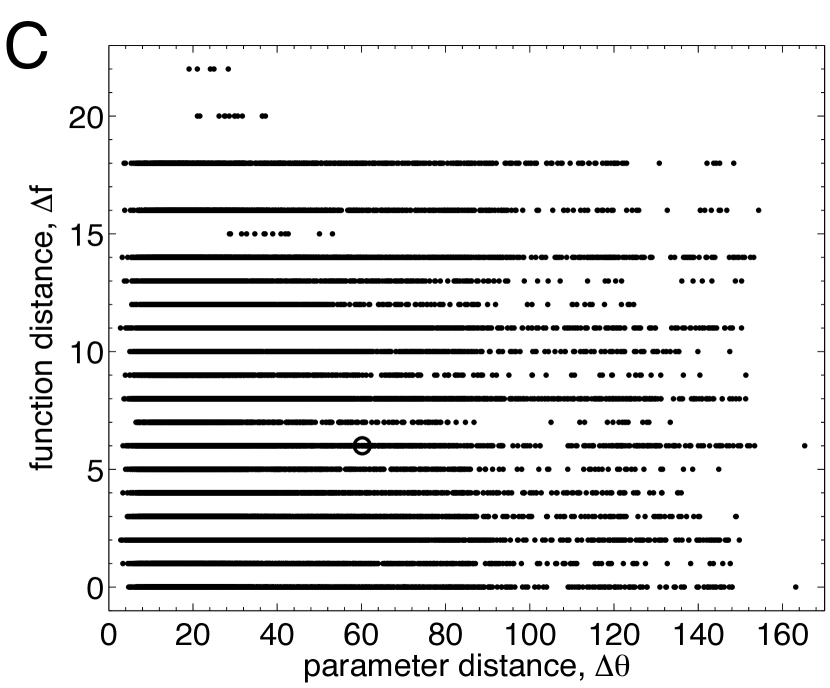
Function distance $\Delta f$ vs. parameter distance $\Delta\theta$ for all pairs of model solutions is plotted in Figure 1C for the example network in Figure 1A. The evolvability score calculated from these data is $E=0.482$ which, since there is little correlation (or anti-correlation) between $\Delta f$ and $\Delta\theta$ in this case, is near the middle value $E=0.5$.

We obtain a fairer estimate of $E$ and an estimate of its error by subsampling. Specifically, in the spirit of Strong et al. Strong et al. (1998), we compute the mean $\bar{E}$ and standard error $\delta E$ in $E$ values calculated on randomly drawn subsets of a given size $n$ (from the full data set of size $N$). We then repeat for various $n$, plot $\bar{E}\pm\delta E$ vs. $N/n$, and fit with a line (all plots generated were roughly linear). The value and uncertainty of the $N/n=0$ intercept give an estimate of $E$, extrapolated to infinite data, and a measure of sampling error, respectively. The sampling error estimated in this way for the data in Figure 1C is $0.001$.

             

Figure 1: Defining evolvability. A Top: a sample regulatory network (see Figure 2 for diagrams of all 24 networks studied). $A$, $B$, and $C$ are genes whose transcription factors regulate each other’s expression according to the given network topology, and $G$ is a “reporter” gene, such as GFP. Sharp arrows indicate up-regulation, while blunt arrows indicate down-regulation (all arrows are blunt in this network). $s_{A}$, $s_{B}$, and $s_{C}$ are chemical inducers that reduce the efficacy of the corresponding transcription factors. Bottom: Table showing the 8 input states $i$ that are defined by the presence or absence of each chemical inducer in the cell ($+$ indicates presence, $-$ indicates absence). In the model, the $s_{A}$, $s_{B}$, and $s_{C}$ are scale factors that are free parameters (greater than 1, to effect an interference with transcriptional regulation) if the inducer is present, and are set to 1 if the inducer is absent. B: Two maximally informative functions performed by the sample network at two different parameter settings. Function is characterized by the order of the output distributions $P(G|i)$, the probability of expressing $G$ proteins per cell given that the system is in input state $i$. Specifically, the function is quantified by the vector $\vec{r}$ of ranks of the $P(G|i)$, as shown for each function in the upper right corner. For example, in the top function, the first output distribution ($i=1$) is ranked $4$th, the second ($i=2$) is ranked $7$th, the third ($i=3$) is ranked $1$st, and so on, so the rank vector is $\vec{r}=(4,7,1,\dots)$. C: Plot of function distance $\Delta f$ [Eqn. (9)] vs. parameter distance $\Delta\theta$ [Eqn. (8)] for all pairs of maximally informative model solutions ($340$ solutions were used for this network). Function distance is scaled such that the swapping of two adjacent output states from solution one to solution two gives $\Delta f=1$, and parameter distance is scaled such that the doubling of one parameter from solution one to solution two gives $\Delta\theta=1$. The point corresponding to the pair of functions in B is circled. The evolvability score for this network, calculated from these data via Eqn. (10), is $E=0.482\pm 0.001$.

II Results

II.1 All networks studied are evolvable

Using the methods described above, between $200$ and $500$ optimally informative model solutions were obtained, and an evolvability score $E$ was calculated for each of the 24 networks shown on the horizontal axis of Fig. 2. The constraints were set to $\lambda=0.01$ or $0.005$, for an average protein count of $\sim$$100-200$, and $\gamma=0.001$, allowing a maximum of about 3 orders of magnitude between upstream and reporter degradation rates. Solutions with mutual information values below $I=2$ bits were discarded as not transmitting high enough information (for scale, a solution with perfectly overlapping output distributions would have $I=0$ bits, and a solution with 8 perfectly non-overlapping output states would have $I=3$ bits).

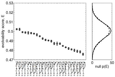
Networks’ evolvability scores are shown in Fig. 2. All 24 networks had $E$ values within $5\%$ of 0.5 (recall that $E$ is bounded by $0\leq E\leq 1$), which means that, in all cases, there is little correlation between change in function and change in parameters, suggesting that all networks studied are evolvable. Using other function distances, including other permutation distances between the rank vectors, and a continuous distance measure defined by averaging the Jensen-Shannon divergence Lin (1991) between corresponding output distributions in the solution pair, produced similar results: $E$ scores were very near $0.5$, indicating little correlation between functional and parametric distances.

The claim that function has little dependence on parameters can be tested more rigorously by comparison with a null hypothesis. The null hypothesis that function is independent of parameters was implemented in two ways. First, given each network’s solution set, locations of solutions in parameter space were kept the same, but the functions associated with each solution were randomly permuted. Second, locations of solutions in parameter space were again kept the same, but functions were drawn randomly from the set of possible functions for each network . In each case, the function reassignment was performed many times, and the $E$ value was computed each time to produce a distribution of null $E$ scores. There was no correlation between the means or variances of the networks’ null distributions and their actual $E$ scores, so the individual null distributions were averaged across networks. Averaged null distributions from each of the two implementations are qualitatively similar, and both are shown in Figure 2. All networks’ actual $E$ values lie well within both null distributions (the smallest $p$-value is $0.023$, and, with 24 networks, we expect at least one to attain a $p$-value lower than $1/24=0.04$ simply by chance). This means that none of the networks’ solution sets significantly differ from a set in which the function performed is independent of the setting of the parameters.

Even though all $E$ values lie within the null distribution, only two lie above the null mean of $0.5$; the probability of this happening by chance is $2\times 10^{-5}$. For a network with $E$ much larger than $0.5$, the parameter and the functional distances would be anti-correlated, and the network function would evolve dramatically with very small parameter changes. Thus the vast majority of the networks studied show a statistically significant, yet unintuitively small, positive correlation among the functional and the parametric distance.

Despite the fact that the $E$ values lie in a narrow range, sampling errors are small (see Fig. 2), meaning that the networks can be ranked with some confidence according to their evolvability. We asked statistically whether this ranking was correlated with any topological features of the network, including the sign of the regulation of each gene, the length and net sign of the feedback cycle, and the total number of activators and repressors in the network, both in and out of the cycle. Correlation was tested for features with categorical values using a Wilcoxon rank-sum test Wilcoxon (1945); Mann and Whitney (1947) (for two categories) or a Kruskal-Wallis $H$-test Kruskal and Wallis (1952) (for more than two categories), and for features with real values using Kendall’s $\tau$ Kendall (1938). No topological feature significantly correlated with $E$. The lowest $p$-value was $0.04$, and, since many correlations were tested for at once, a Bonferoni correction Salkind (2007) showed that the likelihood of obtaining a $p$-value this low simply by chance was $0.33$. Thus we identified no topological aspect that significantly imparted higher or lower evolvability to the networks.

Figure 2: Left: Evolvability scores $E$ for all 24 regulatory networks studied. Networks are shown along the horizontal axis, ranked by $E$ (sharp arrows denote up-regulation, and blunt arrows denote down-regulation). $E$ values are calculated via Eqn. (10), with error bars showing the sampling error, calculated as described in the text. Right: Two null distributions generated according to the null hypothesis that the function distance is independent of the parameter distance. The solid line is the distribution of $E$ scores calculated from solution sets in which the locations in parameter space were held fixed, and the function assignments were randomly permuted. The dotted line is the distribution of $E$ scores calculated from solution sets in which the locations in parameter space were held fixed, and the function assignments were drawn randomly from the set of possible functions for the given network. Both distributions are averages over the individual distributions for each network, as there was no correlation between the means or variances of the individual distributions and the networks’ $E$ scores.

II.2 Changing functions without losing functionality

As described in the previous section, we have found that the networks studied organize their optimally informative solutions in parameter space in such a way that change in function is largely independent of change in parameters. We further demonstrate here that the networks can change from one function to another in parameter space without significant loss of the input-output information along the way. This further underscores the evolvability of these networks, since it shows that random steps in parameter space not only explore the full variety of a network’s functions, but do so without significant loss of fidelity. In the context of electric logical circuits, such evolvability would correspond to an ability to continuously change a logic gate from performing one logical function to another while remaining a functional gate in the interim.

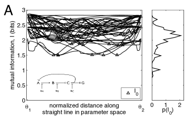
For each network, mutual information $I$ [Eqn. (5)] was calculated along straight-line paths in parameter space between all solutions pairs within a randomly chosen subset of its optimally informative solutions. Examples of these paths are shown in Figure 3A, for $10$ solutions from the inset network. The solutions at either end are local maxima in $I$, and the paths show the loss in information capacity the network would suffer if it were to move from one solution to the other along a straight line in parameter space. Some information loss is unavoidable: changing function requires reordering the output distributions (see Figure 1B), which means overlapping at least two of them at a time, and with $8$ distributions the shift of two distributions from fully separated to fully overlapped incurs a minimum loss of at $0.25$ bits. Seven of the $10$ functions corresponding to the $10$ solutions in Figure 3A are unique; at least $91\%$ of the plotted paths involve a change in function.

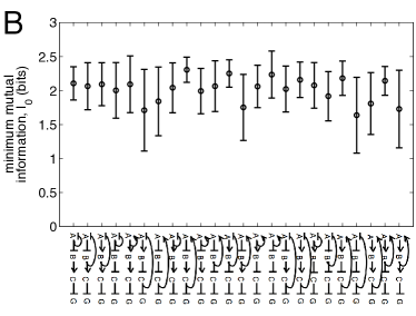
Nonetheless, we find that the loss in information suffered in going between optimal solutions is surprisingly minimal. The right panel of Figure 3A shows the distribution of minimal mutual information values $I_{0}$ along the paths for the inset network, and Figure 3B shows the means and the standard deviations of $I_{0}$ distributions for all networks. For only a few networks do a significant portion of the paths drop below $1.5$ bits, and almost no paths drop below $1$ bit. We note in passing that the networks in Figure 3B are shown as in Figure 2, i.e. ranked by evolvability score $E$, and so Figure 3B also demonstrates that there is no significant correlation between $I_{0}$ and $E$.

We emphasize that Figure 3B represents a lower bound on minimum mutual information encountered in transitioning between solutions. It is by no means necessary (and is most likely biologically unrealistic) for a functional change to proceed via such uniform changes in biochemical parameters. It is more likely that there exist transition paths that are more optimal than the straight-line paths, and that the most optimal $I_{0}$ distributions are actually shifted higher in information than those generated here. Thus it is quite nontrivial (and it is further testament to their evolvability) that even along direct paths between optimal solutions these networks in most cases do not drop below $1.5$ bits of processing ability, considering that the solutions themselves operate in the range of $\sim$$2-2.8$ bits. A network can be evolving and functional at the same time.

      

Figure 3: Changing function without losing information. A Left: Mutual information $I$ along straight-line paths in parameter space between pairs of $10$ randomly chosen optimally informative model solutions for a particular network (inset). For each path, the starting and ending solution’s locations in parameter space are denoted $\vec{\theta}_{1}$ and $\vec{\theta}_{2}$ respectively on the horizontal axis. The minimum mutual information $I_{0}$ along each path is marked with a triangle. A specific function is performed at each of the $10$ solutions (as characterized in Methods); $7$ of the $10$ functions are unique. Right: Distribution of $I_{0}$ values built from paths between $37$ randomly chosen solutions for the inset network, of which the $10$ solutions used for the left plot are a subset. B: Means (circles) and standard deviations (error bars) of $I_{0}$ distributions like that in A (right), for all networks studied; 37 randomly chosen solutions were used to build each network’s distribution. Networks are shown on the horizontal axis, in the same order as in Figure 2, i.e. ranked by evolvability score $E$.

III Discussion

We have quantified the concept of evolvability in the context of regulatory networks by introducing an interpretable measure, and by probing the space of the networks’ most informative functions. Our measure is an anti-correlation between the amount of functional change experienced by a network and the parametric change required to effect it, such that more evolvable networks explore more diverse functions with smaller variation in their biochemical parameters. We have fully defined functional and parametric distances (as well as the characterization of ‘function’ itself) in the context of a stochastic description of the experimental setup of Guet et al. Guet et al. (2002), and we have chosen a correlation measure that is invariant to monotonic transformations in either definition.

We have found that all networks studied share the property that functional change is largely independent of parametric change, meaning that they are highly evolvable by our measure. This property holds for several different definitions of function distance. This means that high-information functions are not organized in parameter space in such a way that similar functions are near each other; instead nearby solutions are approximately as likely to be similar in function as they are to be different in function.

Furthermore, we have found that all networks studied can transition among their maximally informative functions without significant loss of information in the process. Along straight-line paths in parameter space between functions (with mutual information values in the range $\sim$$2-2.8$ bits), mutual information remains above $\sim$$2$ bits on average and very rarely drops below $1$ bit. Moreover, these values represents a lower bound, since transition paths need not be straight. This suggests that the networks can evolve without losing functionality in the process, which resonates with the idea from evolutionary biology that evolution happens not by crossing high fitness barriers (low-information solutions in our case), but by finding neutral paths van Nimwegen and Crutchfield (2000).

Ultimately we have uncovered two important properties of the regulatory networks described by our model: (a) high-information solutions do not cluster by function, and (b) transitions among solutions are possible without significant loss of fidelity. Both of these properties underscore the high evolvability of the networks studied. It is possible that these properties are general characteristics of a class of systems extending beyond small transcriptional regulatory networks, particularly systems governed by a large number of tunable parameters. However, we argue that these properties are especially relevant here, as they are critical to a quantitative description of the capacity of biological networks to evolve.