Scaling properties in deep inelastic scattering

Abstract

Using the “Quality Factor” (QF) method, we analyse the scaling properties of deep-inelastic processes at HERA and fixed target experiments for $x\!\leq\!10^{-2}.$

Geometric scaling [2] is a remarkable empirical property verified by data on high energy deep inelastic scattering (DIS). One can represent with reasonable accuracy the cross section $\sigma^{\gamma^{*}p}$ by the formula $\sigma^{\gamma^{*}p}(Y,Q)=\sigma^{\gamma^{*}}(\tau)\ ,$ where $Q$ is the virtuality of the photon, $Y$ the total rapidity in the ${\gamma^{*}}$-proton system and $\tau=\log Q^{2}-\log Q_{s}(Y)=\log Q^{2}-\lambda Y\$ is the scaling variable. In this paper, we will study different forms of scalings predicted by theory and compare them to the data [3].

scaling	$\partial_{L}T$	$L\partial T/\partial Y$
$T(L-\lambda\sqrt{Y})$	$\frac{\partial T}{\partial L}(L-\lambda\sqrt{Y})=\frac{\partial T}{\partial L}$	$L\frac{\partial T}{\partial Y}=\frac{\lambda L}{2\sqrt{Y}}T$
	SCALING	APPR. SCALING
$T(L-\lambda Y/L$)	$\frac{\partial T}{\partial L}(L-\lambda Y/L)=\left(1+\frac{\lambda Y}{L^{2}}\right)\frac{\partial T}{\partial L}$	$L\frac{\partial T}{\partial Y}(L-\lambda Y/L)=-\lambda\frac{\partial T}{\partial Y}$
	APPR. SCALING	SCALING

Table 1: Approximate scalings in the case of the BK equation (RCI and RCII).

1 Scaling variables

The stochastic extension of the Balitsky-Kovchegov equation [4] for dipole amplitude $T$ reads

$$\frac{\partial T}{\partial Y}=\alpha_{S}\left[\chi(-\partial_{L})T-T^{2}+\sqrt{\alpha_{S}^{2}\kappa T}~{}\nu(L,Y)\right]$$ (1)

where $\chi$ is the BFKL [5] kernel, $L=\log Q^{2}$ and $\nu$ a gaussian “noise” corresponding to the fluctuation of the number of gluons in the proton. The second term of Eq. 1 corresponds to the gluon recombination and the last term to pomeron loops. We notice that we obtain the BFKL LL equation when $\alpha_{S}$ is taken to be constant, the term in $T^{2}$ is neglected and $\kappa=0$ and the Balitsky-Kovchegov equation [4] when $\alpha_{S}$ is constant and $\kappa=0$. Let us consider different cases.

When $\alpha_{S}$ is constant and $\kappa=0$, it is possible to show that the solution of the Balitsky-Kovchegov equation does not depend independently on $Y$ and $\log Q^{2}$ but on a combination of both, $\tau=L-\lambda Y$. This is called “fixed coupling” (FC) in the following.

When $\alpha_{S}$ is running ($\alpha_{S}\sim 1/\log Q^{2}$), it is impossible that both $L\partial T/\partial Y$ and $\chi(-\partial_{L})T$ follow the same scaling at the same time. Two approximate solutions are found either in $T(L-\lambda\sqrt{Y})$ or in $T(L-\lambda Y/L)$. In Table 1, we see that both scalings cannot be satisfied at the same time and scaling is only exact when $L\sim\sqrt{Y}$. In the following, we call the two scalings $\tau=L-\lambda\sqrt{Y}$ and $\tau=L-\lambda Y/L$, “Running coupling I” (RCI) and “Running coupling II” (RCII) respectively. An extension of “Running coupling II” (called RCIIbis) was also considered by adding the additional parameters $\Lambda$ and $Y_{0}$ in $Q/\Lambda$ and $Y-Y_{0}$ instead of $Q$ and $Y$ respectively. The third case is when $\alpha_{S}$ is constant, and we introduce the term in $\sqrt{T}$. In that case, it can be shown that the scaling is

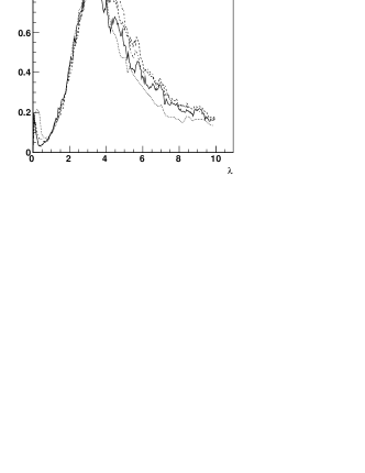
Figure 1: Normalised QF to 1. as a function of $\lambda$ and scaling curve with $\lambda$ fixed to the value corresponding to the best QF for RCII ($\lambda=3.44$). A $Q^{2}>3$ GeV² cut was applied to the data.

$(L-\lambda Y)/\sqrt{Y}$, called diffusive scaling (DS) in the following.

2 Scaling in DIS data

2.1 Quality factor

The question rises how to quantify the quality of the different scalings and compare them using the DIS data. The difficulty comes from the fact that the $\tau$ dependence is not known and an estimator is needed to know whether data points depend only on $\tau$ or not. This is why the concept of quality factor (QF) was introduced [6].

The first step is the normalise the data sets ($F_{2}$ measurements for instance) $v_{i}=\log(\sigma_{i})$ and the scalings $u_{i}=\tau_{i}(\lambda)$ between 0 and 1 . The $u_{i}$ are ordered. We define the QF as

$$QF(\lambda)=\left[\sum_{i}\frac{(v_{i}-v_{i-1})^{2}}{(u_{i}-u_{i-1})^{2}+\epsilon^{2}}\right]^{-1}$$ (2)

where $\epsilon$ is a small term (taken as 0.0001) needed in the case when two data points have the same scaling (same $x$ and $Q^{2}$). The method is then simple: we fit $\lambda$ to maximise QF to obtain the best scaling.

2.2 Scaling tests in DIS using $F_{2}$

To test the different scalings, we first consider the proton structure function measurements $F_{2}$ from H1, ZEUS, NMC and E665 [7]. We apply some cuts on data $1\leq Q^{2}\leq 150$ GeV², $x\leq 10^{-2}$ to stay in the perturbative domain and also avoid the region where valence quark dominates, which leads to 217 data points. As an example, the results for RCII are given in Fig. 1. The different scalings show quite good values of QF, while RCII is favoured and DS disfavoured as it is indicated in Table 2.

scaling	Parameter	QF
FC	$\lambda=-0.33$	1.63
RCI	$\lambda=1.81$	1.62
RCII	$\lambda=3.44$	1.69
RCII bis	$\lambda=3.90$, $\Lambda=0.30$, $Y_{0}=-1.2$	1.82
DS	$\lambda=0.36$	1.44

Table 2: QF for $F_{2}$ data ($Q^{2}>3$ GeV²) and the different scalings. The results are similar when taking all data with $Q^{2}>1$ GeV².

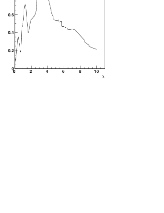
Figure 2: $\lambda$ dependence of the normalised QF to 1. for DVCS data and for RCII. The star indicated the values of $\lambda$ obtained with a fit to $F_{2}$, $Q^{2}>3$ GeV².

To study the $Q^{2}$ dependence of the fitted parameters the data points are divided into four separate $Q^{2}$ samples: $[1;3]$, $[3;10]$, $[10;35]$, and $[35;150]$ GeV². There is a slight increase of the $\lambda$ parameter in the case of FC (from 0.28 to 0.40) while RCI is quite flat at $\lambda\sim 1.8$. This can be easily understood since RCI shows a natural $Q^{2}$ evolution. We notice a stronger increase in the case of RCII ($\lambda$=1.6; 3.2; 3.5; 4.1 in the different $Q^{2}$ regions) , showing the breaking of this scaling as a function of $Q^{2}$. Since this scaling gives already the best QF, it would be worth to study the breaking of scaling and introduce it in the model to further improve the description of the data. The $\lambda$ parameter decreases strongly (especially in the last $Q^{2}$ bin) for the DS from 0.46 to 0.11 which confirms the fact that this scaling leads to the worst description of the data.

We also tested that the $F_{2}^{c}$ from charm data shows the same scalings as for $F_{2}$. However the $F_{2}^{c}$ MRST and CTEQ parametrisations corresponding to NLO QCD DGLAP fits do not show the same scaling, which shows a different behavour between data and parametrisation [3].

2.3 Fits to DVCS data from H1 and ZEUS

After fitting all H1 and ZEUS $F_{2}$ data, it is worth studying whether the DVCS data measured by the same experiments [8] lead to the same results. The amount of data is smaller (34 points for H1 and ZEUS requiring $x\leq 0.01$ as for $F_{2}$ data) and the precision on the $\lambda$ parameter will be weaker. The results of the fits can be found in Fig. 2. To facilitate the comparison between the results of the fits to $F_{2}$ and DVCS data, a star is put at the position of the $\lambda$ value fitted to the H1+ZEUS $F_{2}$ data with $Q^{2}$ in the range $[3;150]$ GeV². We note that the DVCS data lead to similar $\lambda$ values to the $F_{2}$ data, showing the consistency of the scalings.

2.4 Implications for Diffraction and Vector Mesons

In this section, we check if the scalings found in the previous section can also describe diffractive and vector meson data. Since these data are much less precise than the $F_{2}$ or DVCS data and depend more on non-perturbative inputs (meson wave function, diffractive parton distribution inputs…), we choose to impose the same values of parameters found in the previous section and check if the scaling is also observed using this value. Concerning the diffractive $F_{2}^{D}$ data [9], we use $\beta d\sigma_{diff}^{\gamma^{*}\rightarrow Xp}$, and the same definition of $\tau$, replacing $x$ by $x_{I\!\!P}$, $Q^{2}$ remaining the same. For vector meson data [10], we use the same scaling formulae as before replacing $Q^{2}$ by $Q^{2}+M_{V}^{2}$ where $M_{V}$ is the mass of the vector meson. Both data sets show the same scalings as for $F_{2}$, and the quality factors are similar [3]. As an example, we give the scaling curves for $\rho$ data and the fixed coupling scaling in Fig. 3.

As a phenomenological outlook, it seems useful to work out models dipole amplitude which could incorporate the successful scaling laws. On the theoretical ground, our phenomenological analysis can help to improve the theoretical analysis of scaling.

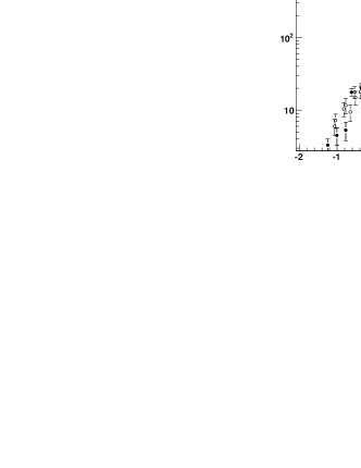
Figure 3: Scaling curves for FC and $\rho$ data using the same $\lambda$ parameter as for the $F_{2}$ fit.

References

-
[1]
Slides:
http://indico.cern.ch/contributionDisplay.py?contribId=184&sessionId=17&confId=24657 - [2] A. M. Staśto, K. Golec-Biernat, and J. Kwiecinski, Phys. Rev. Lett. 86, 596 (2001); K. Golec-Biernat and M. Wusthoff, Phys. Rev. D 59, 014017 (1999).
- [3] G. Beuf, R. Peschanski, C. Royon, D. Salek, arXiv:0803.2186 and references therein; G. Beuf, arXiv:0803.2167.
- [4] I. Balitsky, Nucl. Phys. B 463, 99 (1996); Y. V. Kovchegov, Phys. Rev. D 61, 074018 (2000).
- [5] L. N. Lipatov, Sov. J. Nucl. Phys. 23 (1976) 338; E. A. Kuraev, L. N. Lipatov and V. S. Fadin, Sov. Phys. JETP 45 (1977) 199; I. I. Balitsky and L. N. Lipatov, Sov. J. Nucl. Phys. 28 (1978) 822.
- [6] F. Gelis, R. Peschanski, G. Soyez, L. Schoeffel, Phys. Lett. B 647, 376 (2007); C. Marquet, L. Schoeffel, Phys. Lett. B 639, 471 (2006).
- [7] C. Adloff et al., Eur. Phys. J. C 30 (2003) 1; J. Breitweg et al., Phys. Lett. B 487 (2000) 273; S. Chekanov et al., Phys. Rev. D 70 (2004) 052001; M. Arneodo et al., Nucl. Phys. B 483 (1997) 3; M. R. Adams et al., Phys. Rev. D 54 (1996) 3006.
- [8] A. Aktas et al., Phys. Lett. B659 (2008) 796-806;
- [9] A. Aktas et al., Eur. Phys. J. C 48 (2006) 715-748; S. Chekanov et al., Nucl. Phys. B 713 (2005) 3-80.
- [10] S. Chekanov et al., Nucl. Phys. B 718 (2005) 3-31; A. Aktas et al., Eur. Phys. J. C 46 (2006) 585-603.