Variational Approach to the Chiral Phase Transition
in the Linear Sigma Model

Abstract

The chiral phase transition at finite temperature is investigated in the linear sigma model, which is regarded as a low energy effective theory of QCD with three momentum cutoff, in the variational method with the Gaussian approximation in the functional Schrödinger picture. It is shown that the Goldstone theorem is retained and the meson pair excitations are automatically included by taking into account the linear response to the external fields. It is pointed out that the behavior of chiral phase transition depends on the three-momentum cutoff, which leads to the careful treatment of the problem.

1 Introduction

It is well known that the chiral symmetry plays an essential role in the quark and hadronic world governed by the quantum chromodynamics (QCD). Especially, the spontaneous chiral symmetry breaking leads to the existence of the pion,[1] which plays an important role in the nuclear and hadron physics. One of the recent interests in the hadron physics is the chiral symmetry restoration in the context of the BNL Relativistic Heavy Ion Collider (RHIC) and/or the CERN Large Hadron Collider (LHC).[2] It is believed that the chiral symmetry is restored in the high temperature and/or high baryon density, which might or may be created in the above mentioned experiments.

The finite temperature phase transition in the field theoretical treatment was investigated in the context of the phase transition in the early universe.[3] Systematically, the field theoretical treatment for the systems at finite temperature was developed in the early stage.[4, 5] Further, another approach[6] to the finite temperature systems was devised with the variational technique in terms of the functional Schrödinger picture with Gaussian approximation[7, 8] for the bosonic field theory. In this paper, we intend to adopt a slight different variational approach to the bosonic field theory at finite temperature.

As for the low energy region of the strong interaction, the low energy effective theories of QCD give very useful tool until now to understand the physics of hadrons, especially, based on the chiral symmetry, while the lattice QCD simulation is developed for the problems related to the chiral symmetry. In the low energy region of QCD, the pion and its chiral partner, namely sigma meson, are important ingredients. As an effective theory of QCD, the linear sigma model[9] gives a powerful tool to understand the many properties of low energy hadron physics, which contains pions and sigma meson paying an attention to the chiral symmetry.

In the linear sigma model, the chiral phase transition at finite temperature was firstly investigated in Ref.BG, in which approximations developed in the many-body theory were used widely. However, according to the approximations, the order of the chiral phase transition was not settled definitely. Recently, in the context of the relativistic high energy heavy ion collision experiments, the renewed interests are pointed to the chiral phase transition in the O(N) linear sigma model from the theoretical sides.[11, 12] In the variational approach to the O(N) linear sigma model, it has been pointed out that the Goldstone theorem[13] is not retained in naive treatments. For solving this problem, some works have been carried out.[14, 15, 16, 17] Also, one of the present authors (Y.T.) with Vautherin and Matsui gives another method to recover the Goldstone theorem in the variational approach to the O(N) linear sigma model, in which to take into account the linear response for the external fields is essential.[18]

As for the subject of the chiral phase transition at finite temperature, in Ref.CH, so-called optimized perturbation theory is constructed for the O(N) linear sigma model, in which a certain resummation of the higher order terms is carried out. In the case $N=4$ for the realistic world, the Goldstone theorem is satisfied in this approach and it has been shown that this approach has revealed the second order chiral phase transition at finite temperature with realistic pion mass. On the other hand, the first order phase transition occurs with low pion mass including the case of the chiral limit. Another approach to the same subject was given in Ref.RM which gave a self-consistent Hartree approximation for meson mass equations for one-loop effective potential. Both approaches are carried out the renormalization procedure because the O(N) linear sigma model is renormalizable.

As another approach, the large $N$ limit gives interesting features for O(N) linear sigma model. At zero temperature, the vacuum stability was first investigated.[19] For large $N$ limit in the O(N) linear sigma model, the Goldstone theorem is not broken. In the context of the chiral restoration, the large $N$ approach was investigated and the order of phase transition is discussed[20] by using of the Cornwall-Jackiw-Tomboulis (CJT) effective potential.[21]

In this paper, we investigate the chiral phase transition at finite temperature based on the time-dependent variational approach with Gaussian wave functional and with the imaginary time formalism of Green’s functions,[22] in which the linear responses for the external fields are taken into account. At zero temperature, it has already been shown that the Goldstone theorem is retained in our approach for the O(N) linear sigma model with $N=4$ mentioned above.[18] In this paper, we extend this approach to the finite temperature case and show the behavior of the chiral phase transition. We regard the O(4) linear sigma model as a low energy effective model of QCD, so we introduce the three momentum cutoff parameter $\Lambda$ which cuts the ultraviolet divergences of the meson loop appearing in our approach. It is shown that the pion-pion, pion-sigma meson and sigma-sigma mesons pair excitations are automatically included in our approach, which results to the Goldstone theorem and leads to the second order chiral phase transition with a reasonable parameterization in the O(4) linear sigma model.

This paper is organized as follows: In the next section, we recapitulate the basic ingredients of the variational approach with the linear response for the external fields to the O(N) linear sigma model. The pion and the sigma meson masses are given and it is shown that the meson pair excitations are automatically taken into account. In §3, we extend this approach to the finite temperature system in the Matsubara formalism.[22] In §4, some numerical results and discussion are given. The last section is devoted to a summary and concluding remarks.

2 Variational approach to the $O(4)$ linear sigma model satisfying the Goldstone theorem

In this section, we recapitulate the basic ingredients of the variational method to the O(N) linear sigma model with the Gaussian wave functional and with the polarization tensors appearing in the linear response theory for the external fields.

2.1 Variational approach and the breaking of the Goldstone theorem

We summarize the time-dependent variational method following the Refs.TVM99 and TVM00.

Let us start with the following Hamiltonian of the O(4) linear sigma model with the explicit symmetry breaking term:

$${\cal H}({\mib x})={\cal H}_{0}({\mib x})-c\varphi_{a}({\mib x})\delta_{a0}\ ,$$

$${\cal H}_{0}({\mib x})=\frac{1}{2}\pi_{a}({\mib x})\pi_{a}({\mib x})+\frac{1}{2}\nabla\varphi_{a}({\mib x})\!\cdot\!\nabla\varphi_{a}({\mib x})+\frac{1}{2}m_{0}^{2}\varphi_{a}({\mib x})\varphi_{a}({\mib x})+\frac{\lambda}{24}(\varphi_{a}({\mib x})\varphi_{a}({\mib x}))^{2}\ .$$

Here, $a$ runs from 0 to 3, where $\varphi_{0}$ means the sigma field operator and $\varphi_{i}$ with $i=1\sim 3$ mean the pion field operators. In this paper, we adopt the time-dependent variational approach in the functional Schrödinger picture. In this picture, the conjugate operators $\pi_{a}({\mib x})$ are replaced by the functional derivative $\pi_{a}({\mib x})=-i\delta/\delta\varphi_{a}({\mib x})$. A possible trial wave functional including the quantum fluctuations is a Gaussian wave functional which is written as

$$\Psi[\varphi]=\langle{\varphi}|\Psi\rangle={\cal N}e^{i\langle{\bar{\pi}}|\varphi-{\bar{\varphi}}\rangle}e^{-\langle{\varphi-{\bar{\varphi}}}|\frac{1}{4G}+i\Sigma|{\varphi-{\bar{\varphi}}}\rangle}\ ,$$ (2)

where we used abbreviated notation as $\langle{\bar{\pi}}|\varphi\rangle=\int d^{3}{\mib x}\sum_{a=0}^{3}{\bar{\pi}}_{a}({\mib x},t)\varphi_{a}({\mib x})$ and$\langle{\varphi}|G|{\varphi}\rangle=\int d^{3}{\mib x}d^{3}{\mib y}\sum_{a,b=0}^{3}\varphi_{a}({\mib x})G_{ab}({\mib x},{\mib y},t)\varphi_{b}({\mib y})$. Also, ${\cal N}$ is a normalization factor. Here, the variational functions are ${\bar{\varphi}}_{a}({\mib x},t)$, ${\bar{\pi}}_{a}({\mib x},t)$, $G_{ab}({\mib x},{\mib y},t)$ and $\Sigma_{ab}({\mib x},{\mib y},t)$. In this approach, ${\bar{\varphi}}_{a}$ represent the mean fields and $G_{aa}$ represent the quantum fluctuations around the mean fields ${\bar{\varphi}}_{a}$. The reason why we adopt the above form (2) for the trial state with variational functions ${\bar{\varphi}}_{a}({\mib x},t)$, ${\bar{\pi}}_{a}({\mib x},t)$, $G_{ab}({\mib x},{\mib y},t)$ and $\Sigma_{ab}({\mib x},{\mib y},t)$ is that the $({\bar{\varphi}}_{a}({\mib x},t),{\bar{\pi}}_{a}({\mib x},t))$ and $(G_{ab}({\mib x},{\mib y},t),\Sigma_{ab}({\mib x},{\mib y},t))$ automatically satisfy the canonical variables condition[25] and/or canonicity conditions[26] in terms of the time-dependent Hartree-Fock theory developed in the nuclear many-body theory.

The time-dependence of the variational functions is governed by the following time-dependent variational principle:

$$\delta\int dt\langle{\Psi}|i\frac{\partial}{\partial t}-H|{\Psi}\rangle=0\ ,$$ (3)

where $H=\int d^{3}{\mib x}{\cal H}({\mib x})$. As a result, we derive a basic equation of motion for ${\bar{\varphi}}_{a}({\mib x},t)$:[24]

$$\left(\delta_{ab}\partial_{\mu}\partial^{\mu}+m_{ab}^{2}(x)-\frac{\lambda}{3}{\bar{\varphi}}_{a}{\bar{\varphi}}_{b}\right){\bar{\varphi}}_{b}=c\delta_{a0}\ ,$$ (4)

where we can eliminate ${\bar{\pi}}$ due to the honor of the canonicity condition for ${\bar{\varphi}}$ and ${\bar{\pi}}$. Here, the “mass” function $m_{ab}^{2}(x)$ are defined by

$$m_{ab}^{2}(x)=\left(m_{0}^{2}+\frac{\lambda}{6}{\bar{\varphi}}^{2}+\frac{\lambda}{6}{\rm tr}\ S^{(0)}(x,x)\right)\delta_{ab}+\frac{\lambda}{3}{\bar{\varphi}}_{a}(x){\bar{\varphi}}_{b}(x)+\frac{\lambda}{3}S_{ab}^{(0)}(x,x)\ .\qquad$$ (5)

The function $S^{(0)}_{ab}(x,y)$ corresponds to the propagator and is formally obtained as

$$S^{(0)}(x,y)=\int\frac{d^{4}p}{(2\pi)^{4}}S^{(0)}(p)e^{ip(x-y)}\ ,$$

$$S^{(0)}(p)=\frac{i}{-p^{2}+m^{2}(x)-i\epsilon}$$ (6)

The solution of the variational equation for $G_{aa}({\mib x},{\mib x},t)$ is given in terms of the diagonal element of the above propagator as

$$G_{aa}({\mib x},{\mib x},t)\equiv G(m_{aa}^{2}) = S_{aa}^{(0)}(x,x)\ .$$ (7)

In the Hamiltonian, the direction of the spontaneous chiral symmetry breaking is taken in the sigma direction. Thus, the solution of the mean filed ${\bar{\varphi}}$ is assumedas

$${\bar{\varphi}}={\bar{\varphi}}^{(0)}=\left(\begin{array}[]{@{\,}c@{\,}}\varphi_{0}\\ 0\\ 0\\ 0\end{array}\right)\ .$$ (8)

Then, we define the sigma meson mass $M$ and the pion mass $\mu$, which correspond to the masses derived in the Hartree approximation, as

$$M^{2}=m_{00}^{2}=m_{0}^{2}+\frac{\lambda}{2}\varphi_{0}^{2}+\frac{\lambda}{2}G(M^{2})+\frac{\lambda}{2}G(\mu^{2})\ ,$$

$$\mu^{2}=m_{11}^{2}=m_{22}^{2}=m_{33}^{2}=m_{0}^{2}+\frac{\lambda}{6}\varphi_{0}^{2}+\frac{\lambda}{6}G(M^{2})+\frac{5}{6}\lambda G(\mu^{2})\ .$$ (9)

From (4) in the static case, we can determine the chiral condensate $\varphi_{0}$ by means of the mean filed approximation:

$$\left(M^{2}-\frac{\lambda}{3}\varphi_{0}^{2}\right)\varphi_{0}=c\ .$$ (10)

The solution of the above equation is given in the two phases up to the order of $c$:

$$\frac{\lambda}{3}\varphi_{0}^{2}\approx M^{2}-\sqrt{\frac{\lambda}{3}}\frac{c}{M}\ ,\qquad(\hbox{\rm chiral\ broken\ phase})$$ (11)

$$\varphi_{0}\approx\frac{c}{M^{2}}\ .\qquad(\hbox{\rm chiral\ symmetric\ phase})$$ (12)

It should be noted here that the mass $\mu$ which corresponds to the pion mass does not satisfy the Goldstone theorem in the chiral limit, namely, even if $c=0$, then $\mu\neq 0$.

2.2 Pion mass and recovery of the Goldstone theorem

To see that the Goldstone theorem is satisfied in the variational approach, we introduce the external source field $J_{a}$ coupled with the $\varphi_{a}$:

$${\cal H}^{\prime}={\cal H}-\sum_{a}J_{a}\varphi_{a}\ .$$ (13)

By this source term $J_{a}\varphi_{a}$, the various quantities obtained in the previous subsection are modified as follows:

$${\bar{\varphi}}\longrightarrow{\bar{\varphi}}+\delta\varphi\ ,$$

$$m^{2}(x)\longrightarrow m^{2}(x)+\delta m^{2}\ ,$$

$$S(x,x)\longrightarrow S^{(0)}(x,x)+\delta S(x,x)\ .$$ (14)

As a result, the equation of motion for ${\bar{\varphi}}$ is recast into the equation of motion for $\delta\varphi$ as

$$\left[-q^{2}\delta_{ab}+m_{ab}^{2}(x)-\frac{\lambda}{3}{\bar{\varphi}}_{a}^{(0)}\times{\bar{\varphi}}_{b}^{(0)}\right]\delta\varphi_{b}+\delta m_{ab}^{2}(x){\bar{\varphi}}_{b}^{(0)}$$

$$\qquad\qquad\qquad\qquad-\frac{\lambda}{3}\left(\delta\varphi_{a}\times{\bar{\varphi}}_{b}^{(0)}+{\bar{\varphi}}_{a}^{(0)}\times\delta\varphi_{b}\right){\bar{\varphi}}_{b}^{(0)}=J_{a}\ ,$$ (15)

where ${\bar{\varphi}}_{a}^{(0)}$ is a solution of Eq.(4) and

$$\delta m_{ab}^{2}(x)=\left(\frac{\lambda}{3}\varphi_{0}\delta\varphi_{0}+\frac{\lambda}{6}{\rm tr}\ \delta S\right)\delta_{ab}+\frac{\lambda}{3}\left({\bar{\varphi}}_{a}\times\delta\varphi_{b}+\delta\varphi_{a}\times{\bar{\varphi}}_{b}\right)+\frac{\lambda}{3}\delta S_{ab}\ .$$ (16)

Hereafter, we consider the case that the source field $J_{a}$ has the following form:

$$J_{a}(x)=\varepsilon\delta_{ai}e^{i(\omega t-{\bf q}\cdot{\bf x})}\ .$$ (17)

Then, the shifted quantities $\delta m^{2}$ and $\delta S$ as well as $\delta\varphi$ have the same time- and coordinate-dependence as $J_{a}$:

$$\delta m_{ab}^{2}(x)=\delta{\hat{m}}_{ab}^{2}e^{i(\omega t-{\bf q}\cdot{\bf x})}\ ,$$ (18)

$$\delta S_{ab}(x,x)=\delta{\hat{m}}_{ab}^{2}\Pi_{ab}^{({\rm pol})}(q^{2})e^{i(\omega t-{\bf q}\cdot{\bf x})}\ .$$ (19)

Here, we have defined the polarization tensor $\Pi_{ab}^{({\rm pol})}(q^{2})$ as

$$\Pi_{ab}^{({\rm pol})}(q^{2})=-\int\frac{d^{4}p}{i(2\pi)^{4}}S_{aa}^{(0)}(p+q)S_{bb}^{(0)}(p)\ .$$ (20)

Here, let us consider the pion mass which should satisfy the Goldstone theorem in the chiral limit. In order to derive the pion mass in the variational approach with external fields, we investigate the response of the following external source field:

$$J_{a}(x)=\varepsilon\delta_{a1}e^{i(\omega t-{\bf q}\cdot{\bf x})}\ .$$ (21)

For this source field, only $\delta\varphi_{1}$ responds, namely,

$$\delta\varphi_{1}\neq 0\ ,\qquad\delta\varphi_{a}=0\quad(a=0,2,3)\ .$$ (22)

We take an ansatz for the structure of matrices $\delta m_{ab}$ and $\delta S_{ab}$:

$$\delta m_{ab}^{2}(x)=\left(\begin{array}[]{@{\,}cccc@{\,}}0&\eta&0&0\\ \eta&0&0&0\\ 0&0&0&0\\ 0&0&0&0\end{array}\right)\ ,\qquad\delta S_{ab}(x)=\left(\begin{array}[]{@{\,}cccc@{\,}}0&\delta S&0&0\\ \delta S&0&0&0\\ 0&0&0&0\\ 0&0&0&0\end{array}\right)\ .$$ (23)

It will be understood later that this ansatz is correct.

For $a=1$, we derive the equation of motion from (2.2) as

$$(-q^{2}+\mu^{2})\delta\varphi_{1}+\delta m_{10}^{2}\varphi_{0}-\frac{\lambda}{3}\varphi_{0}^{2}\delta\varphi_{1}=J_{1}\ ,$$ (24)

where

$$\delta m_{10}^{2}=\frac{\lambda}{3}\varphi_{0}\delta\varphi_{1}+\frac{\lambda}{3}\delta S_{10}\ .$$ (25)

From (19) and (25), we obtain

$$\delta m_{10}^{2}\varphi_{0}=\frac{\lambda}{3}\varphi_{0}^{2}\cdot\frac{1}{1-\frac{\lambda}{3}\Pi_{01}^{({\rm pol})}(q^{2})}\cdot\delta\varphi_{1}\ .$$ (26)

Thus, from (24) and the above relation, we can derive the equation of motion for $\delta\varphi_{1}$ under the source field $J_{1}$:

$$\left(-q^{2}+\mu^{2}+\frac{\lambda}{3}\varphi_{0}^{2}\cdot\frac{\frac{\lambda}{3}\Pi_{01}^{({\rm pol})}(q^{2})}{1-\frac{\lambda}{3}\Pi_{01}^{({\rm pol})}(q^{2})}\right)\delta\varphi_{1}=J_{1}\ .$$ (27)

The full propagator $S_{ab}(x,y)$ is thus defined as

$$\delta\varphi_{a}(x)/\delta J_{b}(y)=S_{ab}(x,y)\ .$$ (28)

Then, the mass is defined as the pole of the full propagator:

$$M_{\pi}^{2}=\mu^{2}+\frac{\lambda}{3}\varphi_{0}^{2}\cdot\frac{\frac{\lambda}{3}\Pi_{01}^{({\rm pol})}(0)}{1-\frac{\lambda}{3}\Pi_{01}^{({\rm pol})}(0)}$$ (29)

This mass corresponds to the pion mass. From Eq.(20), the polarization tensor $\Pi_{01}^{({\rm pol})}(q^{2})$ appearing in Eq.(27) or (29) reveals the pion and the sigma meson pair excitation, which is shown in Fig.1 diagrammatically.

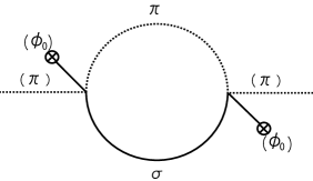
Figure 1: The polarization tensor $\Pi_{01}^{({\rm pol})}$ is depicted diagrammatically. Here, $\Pi_{01}^{({\rm pol})}$ means a part which is gotten rid of the external line $(\pi)$ and the chiral condensate ${\varphi}_{0}$ $(\phi_{0})$ in the above diagram.

Let us try to derive more explicit form for the pion mass $M_{\pi}$. From (7) and (2.1), the following relation is satisfied:

$$G(M^{2})-G(\mu^{2})=\int\frac{d^{4}p}{(2\pi)^{4}}\left(\frac{i}{-p^{2}+M^{2}-i\epsilon}-\frac{i}{-p^{2}+\mu^{2}-i\epsilon}\right)$$ (30)

Thus, the polarization tensor $\Pi_{01}^{({\rm pol})}$ can be expressed as

$$\Pi_{01}^{({\rm pol})}(0)=\frac{G(M^{2})-G(\mu^{2})}{M^{2}-\mu^{2}}\ .$$ (31)

From Eqs.(2.1) and (11) or (12), the following relations are derived easily:

$$\mu^{2}=\sqrt{\frac{\lambda}{3}}\frac{c}{M}-\frac{\lambda}{3}(G(M^{2})-G(\mu^{2}))\ ,\qquad(\hbox{\rm chiral\ broken\ phase})$$ (32)

$$\mu^{2}=M^{2}-\frac{\lambda c^{2}}{3M^{4}}-\frac{\lambda}{3}(G(M^{2})-G(\mu^{2}))\ .\qquad(\hbox{\rm chiral\ symmetric\ phase})$$ (33)

Thus, we obtain

$$\left(1-\frac{\lambda}{3}\Pi_{01}^{({\rm pol})}(0)\right)\mu^{2}=-\frac{\lambda}{3}M^{2}\Pi_{01}^{({\rm pol})}(0)+\sqrt{\frac{\lambda}{3}}\frac{c}{M}\ ,$$

$$\qquad\qquad\qquad\qquad\qquad\qquad\qquad\qquad\qquad\qquad(\hbox{\rm chiral\ broken\ phase})$$ (34)

$$\left(1-\frac{\lambda}{3}\Pi_{01}^{({\rm pol})}(0)\right)\mu^{2}=\left(1-\frac{\lambda}{3}\Pi_{01}^{({\rm pol})}(0)\right)M^{2}-{\frac{\lambda}{3}}\frac{c^{2}}{M^{4}}\ .$$

$$\qquad\qquad\qquad\qquad\qquad\qquad\qquad\qquad\qquad\qquad(\hbox{\rm chiral\ symmetric\ phase})$$ (35)

Substituting the above relation into (29) and using (2$\cdot$11) or (2$\cdot$12) again, we finally obtain the pion mass in the chiral symmetry broken and chiral symmetric phases as

$$M_{\pi}^{2}=\sqrt{\frac{\lambda}{3}}\frac{c}{M}\ ,\qquad(\hbox{\rm chiral\ broken\ phase})$$ (36)

$$M_{\pi}^{2}=M^{2}-\frac{\lambda c^{2}}{3M^{4}}\ ,\qquad(\hbox{\rm chiral\ symmetric\ phase})\ .$$ (37)

As is expected, in the chiral broken phase, if we take the chiral limit $c=0$, the pion mass is reduced to zero which realizes the Goldstone theorem.[18] As is seen in the polarization tensor $\Pi_{01}^{({\rm pol})}$ in Eq.(20) or in Fig.1, the real pion mass contains the effects of the pion and the sigma meson pair excitations. Also, as is seen from the second term of the right-hand side in Eq.(29), the polarization tensor appears in the denominator, so this meson pair excitation is continuously connected as $1/(1-\lambda\Pi_{01}^{({\rm pol})}/3)=1+\lambda\Pi_{01}^{({\rm pol})}/3+\lambda\Pi_{01}^{({\rm pol})}/3\cdot\lambda\Pi_{01}^{({\rm pol})}/3+\cdots$. Thus, the meson pair excitation is automatically included in our approach and leads to the consistency for the Goldstone theorem.

2.3 Sigma meson mass

In this subsection, we derive the sigma meson mass as is similar to deriving the pion mass in the previous subsection. In order to derive the sigma meson mass, we need to introduce the external source field for the sigma direction

$$J_{a}(x)=\varepsilon\delta_{a0}e^{i(\omega t-{\bf q}\cdot{\bf x})}\ ,$$ (38)

and to see the response of this external field. In this case, only $\delta{\varphi}_{0}$ responds:

$$\delta\varphi_{0}\neq 0\ ,\qquad\delta\varphi_{a}=0\quad(a=1,2,3)\ .$$ (39)

We assume the structure of matrices as

$$\delta m_{ab}^{2}(x)=\left(\begin{array}[]{@{\,}cccc@{\,}}\zeta&0&0&0\\ 0&\eta^{\prime}&0&0\\ 0&0&\eta^{\prime}&0\\ 0&0&0&\eta^{\prime}\end{array}\right)\ ,\qquad\delta S_{ab}(x)=\left(\begin{array}[]{@{\,}cccc@{\,}}\delta S_{\sigma}&0&0&0\\ 0&\delta S_{\pi}&0&0\\ 0&0&\delta S_{\pi}&0\\ 0&0&0&\delta S_{\pi}\end{array}\right)\ .$$ (40)

For $a=0$, we obtain the equation of motion for $\delta\varphi_{0}$ as

$$(-q^{2}+M^{2}-\lambda\varphi_{0}^{2})\delta\varphi_{0}+\delta m_{00}^{2}\varphi_{0}=J_{0}\ ,$$ (41)

where

$$\delta m_{00}^{2}={\lambda}\varphi_{0}\delta\varphi_{0}+\frac{\lambda}{2}\delta S_{\sigma}+\frac{\lambda}{2}\delta S_{\pi}\ ,$$ (42)

$$\delta m_{11}^{2}=\delta m_{22}^{2}=\delta m_{33}^{2}=\frac{\lambda}{3}\varphi_{0}\delta\varphi_{0}+\frac{\lambda}{6}\delta S_{\sigma}+\frac{5}{6}\lambda\delta S_{\pi}\ .$$ (43)

From (41) and (19), we obtain

$$\delta m_{00}^{2}\varphi_{0}=\frac{1+\frac{\lambda}{6}{\overline{\Pi}_{11}(q^{2})}}{1-\frac{\lambda}{2}\Pi_{00}^{({\rm pol})}(q^{2})\left(1+\frac{\lambda}{6}{\overline{\Pi}}_{11}(q^{2})\right)}\cdot\lambda\varphi_{0}^{2}\delta\varphi_{0}\ ,$$ (44)

where we define the reduced polarization tensor as

$${\overline{\Pi}}_{11}(q^{2})=\frac{\Pi_{11}^{({\rm pol})}(q^{2})}{1-\frac{5}{6}\lambda\Pi_{11}^{({\rm pol})}(q^{2})}\ .$$ (45)

As a result, we can obtain the following relation from (41):

$$\left(-q^{2}+M^{2}+{\lambda}\varphi_{0}^{2}\cdot\frac{\frac{\lambda}{2}\Pi_{00}^{({\rm pol})}(q^{2})\left(1+\frac{\lambda}{6}{\overline{\Pi}}_{11}(q^{2})\right)+\frac{\lambda}{6}{\overline{\Pi}}_{11}(q^{2})}{1-\frac{\lambda}{2}\Pi_{00}^{({\rm pol})}(q^{2})\left(1+\frac{\lambda}{6}{\overline{\Pi}}_{11}(q^{2})\right)}\right)\delta\varphi_{0}=J_{0}\ .$$ (46)

Thus, we can derive the sigma meson mass $M_{\sigma}$ as a pole of the full propagator $\delta\varphi_{0}/\delta J_{0}$:

$$M_{\sigma}^{2}=M^{2}+{\lambda}\varphi_{0}^{2}\cdot\frac{\frac{\lambda}{2}\Pi_{00}^{({\rm pol})}(0)\left(1+\frac{\lambda}{6}{\overline{\Pi}}_{11}(0)\right)+\frac{\lambda}{6}{\overline{\Pi}}_{11}(0)}{1-\frac{\lambda}{2}\Pi_{00}^{({\rm pol})}(0)\left(1+\frac{\lambda}{6}{\overline{\Pi}}_{11}(0)\right)}\ .$$ (47)

In this formula, the polarization tensors $\Pi_{11}^{({\rm pol})}$ and $\Pi_{00}^{({\rm pol})}$ are automatically included. Here, $\Pi_{11}^{({\rm pol})}$ and $\Pi_{00}^{({\rm pol})}$ represent the pion-pair and the sigma meson-pair excitation, respectively, as is depicted in Fig.2.

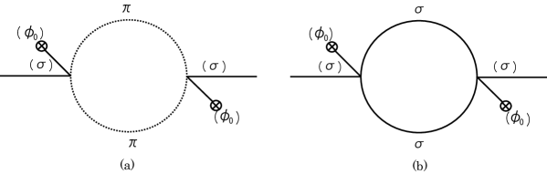
Figure 2: The polarization tensor $\Pi_{11}^{({\rm pol})}$ and $\Pi_{00}^{({\rm pol})}$ are depicted diagrammatically in (a) and (b), respectively. Here, $\Pi_{11}^{({\rm pol})}$ and $\Pi_{00}^{({\rm pol})}$ mean parts which are gotten rid of the external line $(\sigma)$ and the chiral condensate ${\varphi}_{0}$ $(\phi_{0})$ in the above diagrams.

3 Pion and sigma meson masses at finite temperature

In this section, we investigate the pion and sigma meson mass at finite temperature in this variational approach. To extend the method developed in the previous section to the finite temperature case, the $p_{0}$ integral is simply replaced to the Matsubara sum:

$$\int\frac{d^{4}p}{(2\pi)^{4}}f(p)\longrightarrow iT\sum_{n=-\infty}^{\infty}\int\frac{d^{3}{\mib p}}{(2\pi)^{3}}f(i\omega_{n},{\mib p})\ .$$ (48)

Here, $\omega_{n}$ is the Matsubara frequency of the bosons:

$$\omega_{n}=2n\pi T\ .\qquad(n:{\rm integer})$$ (49)

Under this extension, the diagonal element of the propagator is written as

$$S(x,x)=iT\sum_{n=-\infty}^{\infty}\int\frac{d^{3}{\mib p}}{(2\pi)^{3}}S(i\omega_{n},{\mib p})\ ,$$ (50)

where the Fourier transform $S(i\omega_{n},{\mib p})$ is given as

$$S(i\omega_{n},{\mib p})=\frac{i}{\omega_{n}^{2}+{\mib p}^{2}+m^{2}(x)-i\epsilon}\ .$$ (51)

Also, the polarization tensor (20) is rewritten as

$$\Pi_{ab}^{({\rm pol})}(i\omega_{n},{\mib q})=-T\sum_{m=-\infty}^{\infty}\int\frac{d^{3}{\mib p}}{(2\pi)^{3}}S_{aa}(i\omega_{m}+i\omega_{n},{\mib p}+{\mib q})S_{bb}(i\omega_{m},{\mib p})\ .$$ (52)

Using the well-known technique of the contour integral, the sum of the Matsubara frequency is easily taken and the resultant expression for $S(x,x)$ can simply expressed in terms of the bose distribution function $n^{(\pm)}$ as

$$S(x,x)=\frac{1}{4\pi^{2}}\int_{0}^{\infty}d|{\mib p}|\frac{{\mib p}^{2}}{\sqrt{{\mib p}^{2}+m^{2}(x)}}\left(n^{(+)}-n^{(-)}\right)\ ,$$ (53)

$$n^{(\pm)}=\frac{1}{\exp\left(\pm\frac{\sqrt{{\mib p}^{2}+m^{2}(x)}}{T}\right)-1}\ .$$ (54)

Similarly, the polarization tensors at finite temperature are calculated and the results are given as follows:

$$\Pi_{aa}^{({\rm pol})}(0,{\mib 0})=-\frac{1}{8\pi^{2}}\int_{0}^{\Lambda}d|{\mib p}|\frac{{\mib p}^{2}}{{\mib p}^{2}+m_{a}^{2}(x)}$$

$$\qquad\qquad\qquad\times\biggl{[}\frac{1}{T}\left((n_{a}^{(+)})^{2}e^{\sqrt{{\mib p}^{2}+m_{a}(x)^{2}}/T}+(n^{(-)}_{a})^{2}e^{-\sqrt{{\mib p}^{2}+m_{a}(x)^{2}}/T}\right)$$

$$\qquad\qquad\qquad\qquad+\frac{1}{\sqrt{{\mib p}^{2}+m_{a}^{2}(x)}}(n_{a}^{(+)}-(n^{(-)}_{a})\biggl{]}\ ,$$ (55)

$$\Pi_{ab}^{({\rm pol})}(0,{\mib 0})=\frac{1}{4\pi^{2}(m_{a}^{2}-m_{b}^{2})}\int_{0}^{\Lambda}d|{\mib p}|{\mib p}^{2}$$

$$\qquad\qquad\qquad\times\biggl{[}\frac{1}{\sqrt{{\mib p}^{2}+m_{a}^{2}(x)}}(n_{a}^{(+)}-n^{(-)}_{a})-\frac{1}{\sqrt{{\mib p}^{2}+m_{b}^{2}(x)}}(n_{b}^{(+)}-(n^{(-)}_{b})\biggl{]}\ ,$$

$$\qquad\qquad\qquad\qquad\qquad\qquad\qquad\qquad\qquad\qquad\qquad\qquad\qquad\qquad(a\neq b)$$ (56)

where we define $m_{a}=m_{aa}$ and $n_{a}=n_{aa}$ for simplicity.

4 Numerical results and discussion

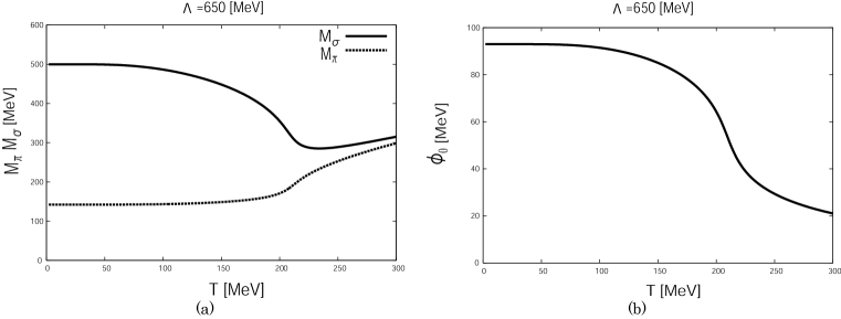
Figure 3: The sigma and pion masses are shown as functions of temperature $T$ in (a). The order parameter of the chiral phase transition $\varphi_{0}$ is depicted in (b). The cutoff parameter $\Lambda$ is taken as 650 MeV.

In this section, we demonstrate the numerical results for the meson masses, $M_{\pi}$ and $M_{\sigma}$, and the mean filed value for $\varphi_{0}$ at finite temperature. The meson masses are given in Eqs.(29) and (47) with the propagator and polarization tensors replaced by Eqs.(50)$\sim$(52) or (53)$\sim$(56) in the finite temperature system. We have model parameters $m_{0}$, $\lambda$, $c$ and the three momentum cutoff $\Lambda$. We take these value to reproduce the pion mass (140 MeV), the sigma meson mass (500 MeV) and the condensate $\varphi_{0}$ (93 MeV) at zero temperature values in each value of $\Lambda$. Here, the three momentum cutoff $\Lambda$ is not determined in this framework. Therefore, we take several values of $\Lambda$.

It is well known that, in the Nambu-Jona Lasinio (NJL) model, the three momentum cutoff is taken as a rather small value around 630 MeV.[23] Thus, we might have to adopt a rather small cutoff value. Under the above consideration, we first take the three momentum cutoff as 650 MeV. Thus, we neglect the polarization tensor $\Pi_{00}^{({\rm pol})}$ because this tensor represents the sigma meson pair excitation. We adopt the sigma meson mass at zero temperature as 500 MeV, so the pair has the energy 1000 MeV at least. This value is beyond the cutoff parameter $\Lambda$. This is the reason why we neglect the polarization tensor $\Pi_{00}^{({\rm pol})}$ in the following numerical calculation. Thus, we set $\Pi_{00}^{({\rm pol})}=0$ in the formula for the sigma meson mass, Eq.(47).

We show the pion and sigma meson masses and the mean field value $\varphi_{0}$ in Fig.3 (a) and (b), respectively. The horizontal axis represents the temperature. In this case, the order parameter, ${\varphi_{0}}$, of the chiral phase transition monotonically decreases and is a single-valued function of the temperature $T$, so the order of phase transition may be likely the second order or crossover. Correspondingly, the pion mass and the sigma meson mass are also monotonically changed and they are single-valued function of $T$.

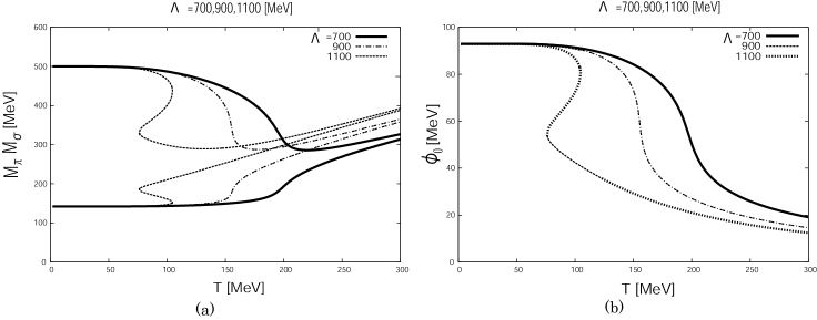
Figure 4: The sigma and pion masses are shown as functions of temperature $T$ in (a). The order parameter of the chiral phase transition $\varphi_{0}$ is depicted in (b). The cutoff parameters $\Lambda$ are taken as 700 MeV (solid curves), 900 MeV (dash-dotted curves) and 1100 MeV (dotted curves), respectively.

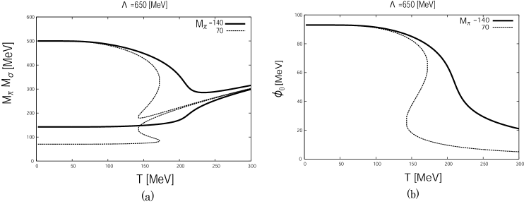
Figure 5: The sigma and pion masses are shown as functions of temperature $T$ in (a). The order parameter of the chiral phase transition $\varphi_{0}$ is depicted in (b). The pion masses at zero temperature are taken as 140 MeV (solid curves) and 70 MeV (dotted curves), respectively. The cutoff parameter $\Lambda$ is taken as 650 MeV.

In Fig.4, we show the results of the pion mass, sigma meson mass and the mean field value of the order parameter $\varphi_{0}$ for the various values of the three momentum cutoff parameter $\Lambda$. Solid curves, dash-dotted curves and the dotted curves show the numerical results for the cutoff parameters $\Lambda=700$ MeV, 900 MeV and 1100 MeV, respectively. If the cutoff parameter $\Lambda$ is taken as a rather larger value, the change of the order parameter is steep in the transition region. Beyond a certain value for $\Lambda$, the order parameter becomes a multi-valued function of $T$. Also, the meson masses become multi-valued functions of $T$. This behavior reveals the first order phase transition. Thus, it should be noted that the choice of the value of cutoff includes subtle problem such as the determination of the order of phase transition. It may be concluded that the rather small value for the cutoff $\Lambda$ should be adopted in this model, because the chiral phase transition at finite temperature may be crossover in the realistic parameterization for the pion mass.

In Fig.5, the dotted curves show the results for the pion mass and sigma meson mass in (a) and the order parameter in (b) with the tree momentum cutoff $\Lambda=650$ MeV, where the pion mass at zero temperature is taken as 70 MeV unrealistically. The solid curves represent the results under the realistic value for zero temperature pion mass for the comparison. For lower pion mass, the order parameter becomes a multi-valued function of the temperature $T$, so the chiral phase transition becomes to the first order one. Thus, in the case of the chiral limit, the chiral phase transition is the first order one within our approach in this O(4) linear sigma model. This behavior is the same as that derived in Ref.CH, where the optimized perturbation theory is used in the same model.

5 Summary and concluding remarks

In this paper, we investigated the chiral phase transition at finite temperature in the O(4) linear sigma model based on the time-dependent variational method devised by the linear response theory for the external fields. In this approach, the Goldstone theorem for the spontaneous chiral symmetry breaking is retained although the variational method is adopted. The reason why the above-mentioned situation is realized is that the meson-pair excitations are automatically included in this approach such as the particle-hole pair excitations for the collective motions of the nuclear many-body problem in the random phase approximation (RPA). It is well known that the pion as a Nambu-Goldstone boson has properties of the collective mode for the quark-antiquark pair in terms of the model based on the quarks.[27]

In the O(4) linear sigma model, the nature of the collective mode is revealed with the pion-sigma meson pair excitations like the RPA in our variational approach devised by the linear response theory. The same situation is realized for the sigma meson which is the chiral partner of the pion in terms of the chiral symmetry. It was shown that the sigma meson contains the effects of the pion-pion and sigma meson-sigma meson pair excitations.

We extended this variational method to the finite temperature case by means of the imaginary time formalism for the finite temperature field theory. This is a natural extension in order to investigate the chiral phase transition at finite temperature.

We have one free model parameter that is the three momentum cutoff parameter $\Lambda$ since we regarded the O(4) linear sigma model as a low energy effective model of QCD. As is similar to the NJL model, we adopted a rather small cutoff $\Lambda$ around 700 MeV. In this parameterization, the order parameter of the chiral phase transition is monotonically changed and is the single-valued function of the temperature $T$. However, the change of the order parameter in the transition region becomes rapid as the cutoff $\Lambda$ is larger. Beyond a certain value of $\Lambda$, the order parameter becomes a multi-valued function of $T$. Thus, it should be noted that the cutoff has to be determined carefully. The similar caution should be given for the pion mass. It was shown that, even if the cutoff parameter is taken as a small value, the order of the chiral phase transition changes according with the pion mass at zero temperature. Thus, the important problem may be to determine the value of cutoff through the physical process, for example, low energy pion-pion scattering, if the O(4) linear sigma model is used as a low energy effective model of QCD. Further, it is well known that a certain susceptibility presents an important information for the chiral phase transition. These investigations are future problems.

Recently, the chiral phase transition at finite temperature is investigated in the same model by using a slight different manner,[28] in which the meson excitations are treated by introducing the Wigner functions and the Vlasov equations are formulated for these Wigner functions.[29] Thus, as another future problem, it may be important to understand the dynamical chiral phase transition in the several situations, for example, in the quench scenario,[30] in the context of the high energy heavy ion collisions.

References

• [1] Y. Nambu and G. Jona-Lasinio, Phys. Rev. 122 (1961), 345: ibid 124 (1961), 246.
• [2] See, for example, Quark-Gluon Plasma 3, eds. by R. C. Hwa and X.-N. Wang (World Scientific, Singapore, 2004).
• [3] D. A. Kirzhnits and A. D. Linde, Phys. Lett. 42B (1972), 471.
• [4] L. Dolan and R. Jackiw, Phys. Rev. D 9 (1974), 3320.
• [5] S. Weinberg, Phys. Rev. D 9 (1974), 3357.
• [6] O. Γ‰boli, R. Jackiw and S.-Y. Pi, Phys. Rev. D 37 (1988), 3557.
R. Jackiw, Physica A 158 (1989), 269.
• [7] R. Jackiw and A. Kerman, Phys. Lett. 71A (1979), 158.
• [8] A. Kerman and D. Vautherin, Ann. Phys. 192 (1989), 408.
• [9] M. Gell-Mann and M. Levy, Nuovo Cim. 16 (1960), 705.
• [10] G. Baym and G. Grinstein, Phys. Rev. D 15 (1977), 2897.
• [11] S. Chiku and T. Hatsuda, Phys. Rev. D 58 (1998), 076001.
• [12] H.-S. Roh and T. Matsui, Eur. Phys. A 1 (1998), 205.
• [13] J. Goldstone, Nuovo Cim. 19 (1961), 154.
• [14] V. DmitraΕ‘inoviΔ‡, J. A. Mcneil and J. R. Shepard, Z. Phys. C 69 (1996), 359.
• [15] A. OkopiΕ„ska, Phys. Lett. B 375 (1996), 213.
• [16] H. Naus, T. Gasenzer and H.-J. Pirner, Ann. Phys. 6 (1997), 287.
• [17] A. Aouissat, G. Chnafray, P. Schuk and J. Wambach, Nucl. Phys. A 603 (1996), 458.
• [18] Y. Tsue, D. Vautherin and T. Matsui, Phys. Rev. D 61 (2000), 076006.
• [19] M. Kobayashi and T. Kugo, Prog. Theor. Phys. 54 (1975), 1537.
• [20] N. Petropoulos, J. Phys. G 25 (1999), 2225.
• [21] J. M. Cornwall, R. Jackiw and E. Tomboulis, Phys. Rev. D 10 (1974), 2428.
• [22] T. Matsubara, Prog. Theor. Phys. 14 (1955), 351.
• [23] T. Hatsuda and T. Kunihiro, Phys. Rep. 247 (1994), 221.
• [24] Y. Tsue, D. Vautherin and T. Matsui, Prog. Theor. Phys. 102 (1999), 313.
• [25] T. Marumori, T. Maskawa, F. Sakata and A. Kuriyama, Prog. Theor. Phys. 64 (1980), 1294.
• [26] M. Yamamura and A. Kuriyama, Prog. Theor. Phys. Suppl. No.93 (1987), 1.
• [27] V. Bernard, R. Brockmann, M. Schaden, W. Weise and E. Werner, Nucl. Phys. A 412 (1984), 349.
• [28] M. Matsuo, private communication.
• [29] T. Matsui and M. Matsuo, Nucl. Phys. A 809 (2008), 211.
• [30] N. Ikezi, M. Asakawa and Y. Tsue, Phys. Rev. C 69 (2004), 032202(R) ; ibid C 73 (2006), 045212.