Stability Bounds for Stationary $\varphi$-mixing and $\beta$-mixing Processes

Abstract

Most generalization bounds in learning theory are based on some measure of the complexity of the hypothesis class used, independently of any algorithm. In contrast, the notion of algorithmic stability can be used to derive tight generalization bounds that are tailored to specific learning algorithms by exploiting their particular properties. However, as in much of learning theory, existing stability analyses and bounds apply only in the scenario where the samples are independently and identically distributed. In many machine learning applications, however, this assumption does not hold. The observations received by the learning algorithm often have some inherent temporal dependence.

This paper studies the scenario where the observations are drawn from a stationary $\varphi$-mixing or $\beta$-mixing sequence, a widely adopted assumption in the study of non-i.i.d. processes that implies a dependence between observations weakening over time. We prove novel and distinct stability-based generalization bounds for stationary $\varphi$-mixing and $\beta$-mixing sequences. These bounds strictly generalize the bounds given in the i.i.d. case and apply to all stable learning algorithms, thereby extending the use of stability-bounds to non-i.i.d. scenarios.

We also illustrate the application of our $\varphi$-mixing generalization bounds to general classes of learning algorithms, including Support Vector Regression, Kernel Ridge Regression, and Support Vector Machines, and many other kernel regularization-based and relative entropy-based regularization algorithms. These novel bounds can thus be viewed as the first theoretical basis for the use of these algorithms in non-i.i.d. scenarios.

Keywords: Mixing Distributions, Algorithmic Stability, Generalization Bounds, Machine Learning Theory

1 Introduction

Most generalization bounds in learning theory are based on some measure of the complexity of the hypothesis class used, such as the VC-dimension, covering numbers, or Rademacher complexity. These measures characterize a class of hypotheses, independently of any algorithm. In contrast, the notion of algorithmic stability can be used to derive bounds that are tailored to specific learning algorithms and exploit their particular properties. A learning algorithm is stable if the hypothesis it outputs varies in a limited way in response to small changes made to the training set. Algorithmic stability has been used effectively in the past to derive tight generalization bounds (Bousquet and Elisseeff, 2001, 2002).

But, as in much of learning theory, existing stability analyses and bounds apply only in the scenario where the samples are independently and identically distributed (i.i.d.). In many machine learning applications, this assumption, however, does not hold; in fact, the i.i.d. assumption is not tested or derived from any data analysis. The observations received by the learning algorithm often have some inherent temporal dependence. This is clear in system diagnosis or time series prediction problems. Clearly, prices of different stocks on the same day, or of the same stock on different days, may be dependent. But, a less apparent time dependency may affect data sampled in many other tasks as well.

This paper studies the scenario where the observations are drawn from a stationary $\varphi$-mixing or $\beta$-mixing sequence, a widely adopted assumption in the study of non-i.i.d. processes that implies a dependence between observations weakening over time (Yu, 1994; Meir, 2000; Vidyasagar, 2003; Lozano et al., 2006). We prove novel and distinct stability-based generalization bounds for stationary $\varphi$-mixing and $\beta$-mixing sequences. These bounds strictly generalize the bounds given in the i.i.d. case and apply to all stable learning algorithms, thereby extending the usefulness of stability-bounds to non-i.i.d. scenarios. Our proofs are based on the independent block technique described by Yu (1994) and attributed to Bernstein (1927), which is commonly used in such contexts. However, our analysis differs from previous uses of this technique in that the blocks of points considered are not of equal size.

For our analysis of stationary $\varphi$-mixing sequences, we make use of a generalized version of McDiarmid’s inequality (Kontorovich and Ramanan, 2006) that holds for $\varphi$-mixing sequences. This leads to stability-based generalization bounds with the standard exponential form. Our generalization bounds for stationary $\beta$-mixing sequences cover a more general non-i.i.d. scenario and use the standard McDiarmid’s inequality, however, unlike the $\varphi$-mixing case, the $\beta$-mixing bound presented here is not a purely exponential bound and contains an additive term depending on the mixing coefficient.

We also illustrate the application of our $\varphi$-mixing generalization bounds to general classes of learning algorithms, including Support Vector Regression (SVR) (Vapnik, 1998), Kernel Ridge Regression (Saunders et al., 1998), and Support Vector Machines (SVMs) (Cortes and Vapnik, 1995). Algorithms such as support vector regression (SVR) (Vapnik, 1998; Schölkopf and Smola, 2002) have been used in the context of time series prediction in which the i.i.d. assumption does not hold, some with good experimental results (Müller et al., 1997; Mattera and Haykin, 1999). To our knowledge, the use of these algorithms in non-i.i.d. scenarios has not been previously supported by any theoretical analysis. The stability bounds we give for SVR, SVMs, and many other kernel regularization-based and relative entropy-based regularization algorithms can thus be viewed as the first theoretical basis for their use in such scenarios.

The following sections are organized as follows. In Section 2, we introduce the necessary definitions for the non-i.i.d. problems that we are considering and discuss the learning scenarios in that context. Section 3 gives our main generalization bounds for stationary $\varphi$-mixing sequences based on stability, as well as the illustration of its applications to general kernel regularization-based algorithms, including SVR, KRR, and SVMs, as well as to relative entropy-based regularization algorithms. Finally, Section 4 presents the first known stability bounds for the more general stationary $\beta$-mixing scenario.

2 Preliminaries

We first introduce some standard definitions for dependent observations in mixing theory (Doukhan, 1994) and then briefly discuss the learning scenarios in the non-i.i.d. case.

2.1 Non-i.i.d. Definitions

Definition 1

A sequence of random variables $\mathbf{Z}=\left\{Z_{t}\right\}_{t=-\infty}^{\infty}$ is said to be stationary if for any $t$ and non-negative integers $m$ and $k$, the random vectors $(Z_{t},\ldots,Z_{t+m})$ and $(Z_{t+k},\ldots,Z_{t+m+k})$ have the same distribution.

Thus, the index $t$ or time, does not affect the distribution of a variable $Z_{t}$ in a stationary sequence. This does not imply independence however. In particular, for $i<j<k$, $\Pr[Z_{j}\mid Z_{i}]$ may not equal $\Pr[Z_{k}\mid Z_{i}]$. The following is a standard definition giving a measure of the dependence of the random variables $Z_{t}$ within a stationary sequence. There are several equivalent definitions of this quantity, we are adopting here that of (Yu, 1994).

Definition 2

Let $\mathbf{Z}=\left\{Z_{t}\right\}_{t=-\infty}^{\infty}$ be a stationary sequence of random variables. For any $i,j\in\mathbb{Z}\cup\left\{-\infty,+\infty\right\}$, let $\sigma_{i}^{j}$ denote the $\sigma$-algebra generated by the random variables $Z_{k}$, $i\leq k\leq j$. Then, for any positive integer $k$, the $\beta$-mixing and $\varphi$-mixing coefficients of the stochastic process $\mathbf{Z}$ are defined as

$$\beta(k)=\sup_{n}\operatorname*{\rm E}_{B\in\sigma_{-\!\infty}^{n}}\Bigl{[}\sup_{A\in\sigma_{n+k}^{\infty}}\Bigl{|}\Pr[A\mid B]-\Pr[A]\Bigr{|}\Bigr{]}\quad\varphi(k)=\sup_{\begin{subarray}{c}n\\ A\in\sigma_{n+k}^{\infty}\\ B\in\sigma_{-\!\infty}^{n}\end{subarray}}\Bigl{|}\Pr[A\mid B]-\Pr[A]\Bigr{|}.$$ (1)

$\mathbf{Z}$ is said to be $\beta$-mixing ($\varphi$-mixing) if $\beta(k)\to 0$ (resp. $\varphi(k)\to 0$) as $k\to\infty$. It is said to be algebraically $\beta$-mixing (algebraically $\varphi$-mixing) if there exist real numbers $\beta_{0}>0$ (resp. $\varphi_{0}>0$) and $r>0$ such that $\beta(k)\leq\beta_{0}/k^{r}$ (resp. $\varphi(k)\leq\varphi_{0}/k^{r}$) for all $k$, exponentially mixing if there exist real numbers $\beta_{0}$ (resp. $\varphi_{0}>0$) and $\beta_{1}$ (resp. $\varphi_{1}>0$) such that $\beta(k)\leq\beta_{0}\exp(-\beta_{1}k^{r})$ (resp. $\varphi(k)\leq\varphi_{0}\exp(-\varphi_{1}k^{r})$) for all $k$.

Both $\beta(k)$ and $\varphi(k)$ measure the dependence of an event on those that occurred more than $k$ units of time in the past. $\beta$-mixing is a weaker assumption than $\varphi$-mixing and thus covers a more general non-i.i.d. scenario.

This paper gives stability-based generalization bounds both in the $\varphi$-mixing and $\beta$-mixing case. The $\beta$-mixing bounds cover a more general case of course, however, the $\varphi$-mixing bounds are simpler and admit the standard exponential form. The $\varphi$-mixing bounds are based on a concentration inequality that applies to $\varphi$-mixing processes only. Except from the use of this concentration bound, all of the intermediate proofs and results to derive a $\varphi$-mixing bound in Section 3 are given in the more general case of $\beta$-mixing sequences.

It has been argued by Vidyasagar (2003) that $\beta$-mixing is “just the right” assumption for the analysis of weakly-dependent sample points in machine learning, in particular because several PAC-learning results then carry over to the non-i.i.d. case. Our $\beta$-mixing generalization bounds further contribute to the analysis of this scenario.

We describe in several instances the application of our bounds in the case of algebraic mixing. Algebraic mixing is a standard assumption for mixing coefficients that has been adopted in previous studies of learning in the presence of dependent observations (Yu, 1994; Meir, 2000; Vidyasagar, 2003; Lozano et al., 2006).

Let us also point out that mixing assumptions can be checked in some cases such as with Gaussian or Markov processes (Meir, 2000) and that mixing parameters can also be estimated in such cases.

Most previous studies use a technique originally introduced by Bernstein (1927) based on independent blocks of equal size (Yu, 1994; Meir, 2000; Lozano et al., 2006). This technique is particularly relevant when dealing with stationary $\beta$-mixing. We will need a related but somewhat different technique since the blocks we consider may not have the same size. The following lemma is a special case of Corollary 2.7 from (Yu, 1994).

Lemma 3 (Yu (Yu, 1994), Corollary 2.7)

Let $\mu\geq 1$ and suppose that $h$ is measurable function, with absolute value bounded by $M$, on a product probability space $\left(\prod_{j=1}^{\mu}\Omega_{j},\prod_{i=1}^{\mu}\sigma_{r_{i}}^{s_{i}}\right)$ where $r_{i}\leq s_{i}\leq r_{i+1}$ for all $i$. Let $Q$ be a probability measure on the product space with marginal measures $Q_{i}$ on ($\Omega_{i},\sigma_{r_{i}}^{s_{i}}$), and let $Q^{i+1}$ be the marginal measure of $Q$ on $\left(\prod_{j=1}^{i+1}\Omega_{j},\prod_{j=1}^{i+1}\sigma_{r_{j}}^{s_{j}}\right)$, $i=1,\ldots,\mu-1$. Let $\beta(Q)=\sup_{1\leq i\leq\mu-1}\beta(k_{i})$, where $k_{i}=r_{i+1}-s_{i}$, and $P=\prod_{i=1}^{\mu}Q_{i}$. Then,

$$|\operatorname*{\rm E}_{Q}[h]-\operatorname*{\rm E}_{P}[h]|\leq(\mu-1)M\beta(Q).$$ (2)

The lemma gives a measure of the difference between the distribution of $\mu$ blocks where the blocks are independent in one case and dependent in the other case. The distribution within each block is assumed to be the same in both cases. For a monotonically decreasing function $\beta$, we have $\beta(Q)=\beta(k^{*})$, where $k^{*}=\min_{i}(k_{i})$ is the smallest gap between blocks.

2.2 Learning Scenarios

We consider the familiar supervised learning setting where the learning algorithm receives a sample of $m$ labeled points $S=(z_{1},\ldots,z_{m})=((x_{1},y_{1}),\ldots,(x_{m},y_{m}))\in(X\times Y)^{m}$, where $X$ is the input space and $Y$ the set of labels ($Y=\mathbb{R}$ in the regression case), both assumed to be measurable.

For a fixed learning algorithm, we denote by $h_{S}$ the hypothesis it returns when trained on the sample $S$. The error of a hypothesis on a pair $z\in X\times Y$ is measured in terms of a cost function $c:Y\times Y\to\mathbb{R}_{+}$. Thus, $c(h(x),y)$ measures the error of a hypothesis $h$ on a pair $(x,y)$, $c(h(x),y)=(h(x)-y)^{2}$ in the standard regression cases. We will use the shorthand $c(h,z):=c(h(x),y)$ for a hypothesis $h$ and $z=(x,y)\in X\times Y$ and will assume that $c$ is upper bounded by a constant $M>0$. We denote by $\widehat{R}(h)$ the empirical error of a hypothesis $h$ for a training sample $S=(z_{1},\ldots,z_{m})$:

$$\widehat{R}(h)=\frac{1}{m}\sum_{i=1}^{m}c(h,z_{i}).$$ (3)

In the standard machine learning scenario, the sample pairs $z_{1},\ldots,z_{m}$ are assumed to be i.i.d., a restrictive assumption that does not always hold in practice. We will consider here the more general case of dependent samples drawn from a stationary mixing sequence $\mathbf{Z}$ over $X\times Y$. As in the i.i.d. case, the objective of the learning algorithm is to select a hypothesis with small error over future samples. But, here, we must distinguish two versions of this problem.

In the most general version, future samples depend on the training sample $S$ and thus the generalization error or true error of the hypothesis $h_{S}$ trained on $S$ must be measured by its expected error conditioned on the sample $S$:

$$R(h_{S})=\operatorname*{\rm E}_{z}[c(h_{S},z)\mid S].$$ (4)

This is the most realistic setting in this context, which matches time series prediction problems. A somewhat less realistic version is one where the samples are dependent, but the test points are assumed to be independent of the training sample $S$. The generalization error of the hypothesis $h_{S}$ trained on $S$ is then:

$$R(h_{S})=\operatorname*{\rm E}_{z}[c(h_{S},z)\mid S]=\operatorname*{\rm E}_{z}[c(h_{S},z)].$$ (5)

This setting seems less natural since, if samples are dependent, future test points must also depend on the training points, even if that dependence is relatively weak due to the time interval after which test points are drawn. Nevertheless, it is this somewhat less realistic setting that has been studied by all previous machine learning studies that we are aware of (Yu, 1994; Meir, 2000; Vidyasagar, 2003; Lozano et al., 2006), even when examining specifically a time series prediction problem (Meir, 2000). Thus, the bounds derived in these studies cannot be directly applied to the more general setting.

We will consider instead the most general setting with the definition of the generalization error based on Eq. 4. Clearly, our analysis also applies to the less general setting just discussed as well.

Let us briefly discuss the more general scenario of non-stationary mixing sequences, that is one where the distribution may change over time. Within that general case, the generalization error of a hypothesis $h_{S}$, defined straightforwardly by

$$R(h_{S},t)=\operatorname*{\rm E}_{z_{t}\sim\sigma_{t}^{t}}[c(h_{S},z_{t})\mid S],$$ (6)

would depend on the time $t$ and it may be the case that $R(h_{S},t)\neq R(h_{S},t^{\prime})$ for $t\neq t^{\prime}$, making the definition of the generalization error a more subtle issue. To remove the dependence on time, one could define a weaker notion of the generalization error based on an expected loss over all time:

$$R(h_{S})=\operatorname*{\rm E}_{t}[R(h_{S},t)].$$ (7)

It is not clear however whether this term could be easily computed and useful. A stronger condition would be to minimize the generalization error for any particular target time. Studies of this type have been conducted for smoothly changing distributions, such as in Zhou et al. (2008), however, to the best of our knowledge, the scenario of a both non-identical and non-independent sequences has not yet been studied.

3 $\varphi$-Mixing Generalization Bounds and Applications

This section gives generalization bounds for $\hat{\beta}$-stable algorithms over a mixing stationary distribution. The first two sections present our main proofs which hold for $\beta$-mixing stationary distributions. In the third section, we will briefly discuss concentration inequalities that apply to $\varphi$-mixing processes only. Then, in the final section, we will present our main results.

The condition of $\hat{\beta}$-stability is an algorithm-dependent property first introduced by Devroye and Wagner (1979) and Kearns and Ron (1997). It has been later used successfully by Bousquet and Elisseeff (2001, 2002) to show algorithm-specific stability bounds for i.i.d. samples. Roughly speaking, a learning algorithm is said to be stable if small changes to the training set do not produce large deviations in its output. The following gives the precise technical definition.

Definition 4

A learning algorithm is said to be (uniformly) $\hat{\beta}$-stable if the hypotheses it returns for any two training samples $S$ and $S^{\prime}$ that differ by a single point satisfy

$$\forall z\in X\times Y,\quad|c(h_{S},z)-c(h_{S^{\prime}},z)|\leq\hat{\beta}.$$ (8)

The use of stability in conjunction with McDiarmid’s inequality will allow us to produce generalization bounds. McDiarmid’s inequality is an exponential concentration bound of the type,

$$\Pr[|\Phi-\operatorname*{\rm E}[\Phi]|\geq\epsilon]\leq\exp\left(-\frac{\epsilon^{2}}{ml^{2}}\right),$$

where the probability is over a sample of size $m$ and $l$ is the Lipschitz parameter of $\Phi$ (which is also a function of $m$). Unfortunately, this inequality cannot be easily applied when the sample points are not distributed in an i.i.d. fashion. We will use the results of Kontorovich and Ramanan (2006) to extend the use of McDiarmid’s inequality with general mixing distributions (Theorem 9).

To obtain a stability-based generalization bound, we will apply this theorem to $\Phi(S)=R(h_{S})-\widehat{R}(h_{S})$. To do so, we need to show, as with the standard McDiarmid’s inequality, that $\Phi$ is a Lipschitz function and, to make it useful, bound $\operatorname*{\rm E}[\Phi]$. The next two sections describe how we achieve both of these in this non-i.i.d. scenario.

Let us first take a brief look at the problem faced when attempting to give stability bounds for dependent sequences and give some idea of our solution for that problem. The stability proofs given by Bousquet and Elisseeff (2001) assume the i.i.d. property, thus replacing an element in a sequence with another does not affect the expected value of a random variable defined over that sequence. In other words, the following equality holds,

$$\operatorname*{\rm E}_{S}[V(Z_{1},\ldots,Z_{i},\ldots,Z_{m})]=\operatorname*{\rm E}_{S,Z^{\prime}}[V(Z_{1},\ldots,Z^{\prime},\ldots,Z_{m})],$$ (9)

for a random variable $V$ that is a function of the sequence of random variables $S=(Z_{1},\ldots,Z_{m})$. However, clearly, if the points in that sequence $S$ are dependent, this equality may not hold anymore.

The main technique to cope with this problem is based on the so-called “independent block sequence” originally introduced by Bernstein (1927). This consists of eliminating from the original dependent sequence several blocks of contiguous points, leaving us with some remaining blocks of points. Instead of these dependent blocks, we then consider independent blocks of points, each with the same size and the same distribution (within each block) as the dependent ones. By Lemma 3, for a $\beta$-mixing distribution, the expected value of a random variable defined over the dependent blocks is close to the one based on these independent blocks. Working with these independent blocks brings us back to a situation similar to the i.i.d. case, with i.i.d. blocks replacing i.i.d. points.

Our use of this method somewhat differs from previous ones (see Yu, 1994; Meir, 2000) where many blocks of equal size are considered. We will be dealing with four blocks and with typically unequal sizes. More specifically, note that for Equation 9 to hold, we only need that the variable $Z_{i}$ be independent of the other points in the sequence. To achieve this, roughly speaking, we will be “discarding” some of the points in the sequence surrounding $Z_{i}$. This results in a sequence of three blocks of contiguous points. If our algorithm is stable and we do not discard too many points, the hypothesis returned should not be greatly affected by this operation. In the next step, we apply the independent block lemma, which then allows us to assume each of these blocks as independent modulo the addition of a mixing term. In particular, $Z_{i}$ becomes independent of all other points. Clearly, the number of points discarded is subject to a trade-off: removing too many points could excessively modify the hypothesis returned; removing too few would maintain the dependency between $Z_{i}$ and the remaining points, thereby producing a larger penalty when applying Lemma 3. This trade-off is made explicit in the following section where an optimal solution is sought.

3.1 Lipschitz Bound

As discussed in Section 2.2, in the most general scenario, test points depend on the training sample. We first present a lemma that relates the expected value of the generalization error in that scenario and the same expectation in the scenario where the test point is independent of the training sample. We denote by $R(h_{S})=\operatorname*{\rm E}_{z}[c(h_{S},z)|S]$ the expectation in the dependent case and by $\widetilde{R}(h_{S_{b}})=\operatorname*{\rm E}_{\widetilde{z}}[c(h_{S_{b}},\widetilde{z})]$ the expectation where the test points are assumed independent of the training, with $S_{b}$ denoting a sequence similar to $S$ but with the last $b$ points removed. Figure 1(a) illustrates that sequence. The block $S_{b}$ is assumed to have exactly the same distribution as the corresponding block of the same size in $S$.

Lemma 5

Assume that the learning algorithm is $\hat{\beta}$-stable and that the cost function $c$ is bounded by $M$. Then, for any sample $S$ of size $m$ drawn from a $\beta$-mixing stationary distribution and for any $b\in\{0,\ldots,m\}$, the following holds:

$$|\operatorname*{\rm E}_{S}[R(h_{S})]-\operatorname*{\rm E}_{S}[\widetilde{R}(h_{S_{b}})]|\leq b\hat{\beta}+\beta(b)M.$$ (10)

Proof  The $\hat{\beta}$-stability of the learning algorithm implies that

$$\operatorname*{\rm E}_{S}[R(h_{S})]=\operatorname*{\rm E}_{S,z}[c(h_{S},z)]\leq\operatorname*{\rm E}_{S,z}[c(h_{S_{b}},z)]+b\hat{\beta}.$$ (11)

The application of Lemma 3 yields

$$\operatorname*{\rm E}_{S}[R(h_{S})]\leq\operatorname*{\rm E}_{S,\widetilde{z}}[c(h_{S_{b}},\widetilde{z})]+b\hat{\beta}+\beta(b)M=\widetilde{\operatorname*{\rm E}}_{S}[R(h_{S_{b}})]+b\hat{\beta}+\beta(b)M.$$ (12)

The other side of the inequality of the lemma can be shown following the same steps.  
We can now prove a Lipschitz bound for the function $\Phi$.

Lemma 6

Let $S=(z_{1},\dots,z_{i},\dots,z_{m})$ and $S^{i}=(z_{1},\dots,z_{i}^{\prime},\dots,z_{m})$ be two sequences drawn from a $\beta$-mixing stationary process that differ only in point $i\in[1,m]$, and let $h_{S}$ and $h_{S^{i}}$ be the hypotheses returned by a $\hat{\beta}$-stable algorithm when trained on each of these samples. Then, for any $i\in[1,m]$, the following inequality holds:

$$|\Phi(S)-\Phi(S^{i})|\leq(b+1)2\hat{\beta}+2\beta(b)M+\frac{M}{m}.$$ (13)

Proof  To prove this inequality, we first bound the difference of the empirical errors as in (Bousquet and Elisseeff, 2002), then the difference of the true errors. Bounding the difference of costs on agreeing points with $\hat{\beta}$ and the one that disagrees with $M$ yields

$$|\widehat{R}(h_{S})-\widehat{R}(h_{S^{i}})| = \frac{1}{m}\sum_{j\neq i}|c(h_{S},z_{j})-c(h_{S^{i}},z_{j})|+\frac{1}{m}|c(h_{S},z_{i})-c(h_{S^{i}},z_{i}^{\prime})|$$

$$\leq \hat{\beta}+\frac{M}{m}.$$

Since both $R(h_{S})$ and $R(h_{S^{i}})$ are defined with respect to a (different) dependent point, we apply Lemma 5 to both generalization error terms and use $\hat{\beta}$-stability. This then results in

$$|R(h_{S})-R(h_{S^{i}})| \leq |\widetilde{R}(h_{S_{b}})-\widetilde{R}(h_{S_{b}^{i}})|+2b\hat{\beta}+2\beta(b)$$

$$= \operatorname*{\rm E}_{\widetilde{z}}[c(h_{S_{b}},\widetilde{z})-c(h_{S_{b}^{i}},\widetilde{z})]+2b\hat{\beta}+2\beta(b)M\leq\hat{\beta}+2b\hat{\beta}+2\beta(b)M.$$

The lemma’s statement is obtained by combining inequalities 3.1 and 3.1.  

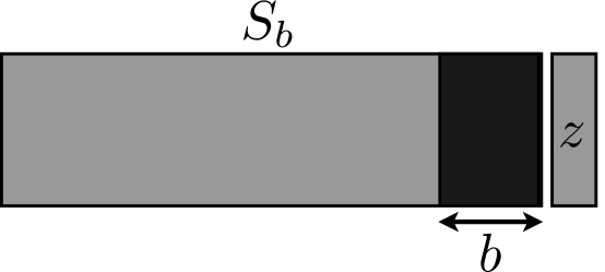
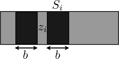
(a)	(b)
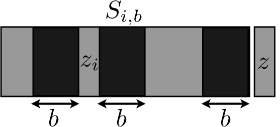
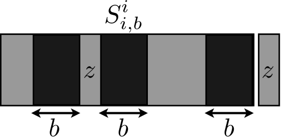
(c)	(d)

Figure 1: Illustration of the sequences derived from $S$ that are considered in the proofs.

3.2 Bound on Expectation

As mentioned earlier, to obtain an explicit bound after application of a generalized McDiarmid’s inequality, we also need to bound $\operatorname*{\rm E}_{S}[\Phi(S)]$. This is done by analyzing independent blocks using Lemma 3.

Lemma 7

Let $h_{S}$ be the hypothesis returned by a $\hat{\beta}$-stable algorithm trained on a sample $S$ drawn from a stationary $\beta$-mixing distribution. Then, for all $b\in[1,m]$, the following inequality holds:

$$\operatorname*{\rm E}_{S}[|\Phi(S)|]\leq(6b+1)\hat{\beta}+3\beta(b)M.$$ (16)

Proof  Let $S_{b}$ be defined as in the proof of Lemma 5. To deal with independent block sequences defined with respect to the same hypothesis, we will consider the sequence $S_{i,b}=S_{i}\cap S_{b}$, which is illustrated by Figure 1(c). This can result in as many as four blocks. As before, we will consider a sequence $\widetilde{S}_{i,b}$ with a similar set of blocks each with the same distribution as the corresponding blocks in $S_{i,b}$, but such that the blocks are independent.

Since three blocks of at most $b$ points are removed from each hypothesis, by the $\hat{\beta}$-stability of the learning algorithm, the following holds:

$$\operatorname*{\rm E}_{S}[\Phi(S)] = \operatorname*{\rm E}_{S}[\widehat{R}(h_{S})-R(h_{S})]=\operatorname*{\rm E}_{S,z}\left[\frac{1}{m}\sum_{i=1}^{m}c(h_{S},z_{i})-c(h_{S},z)\right]$$ (17)

$$\leq \operatorname*{\rm E}_{S_{i,b},z}\left[\frac{1}{m}\sum_{i=1}^{m}c(h_{S_{i,b}},z_{i})-c(h_{S_{i,b}},z)\right]+6b\hat{\beta}.$$ (18)

The application of Lemma 3 to the difference of two cost functions also bounded by $M$ as in the right-hand side leads to

$$\operatorname*{\rm E}_{S}[\Phi(S)]\leq\operatorname*{\rm E}_{\widetilde{S}_{i,b},\widetilde{z}}\left[\frac{1}{m}\sum_{i=1}^{m}c(h_{\widetilde{S}_{i,b}},\widetilde{z}_{i})-c(h_{\widetilde{S}_{i,b}},\widetilde{z})\right]+6b\hat{\beta}+3\beta(b)M.$$ (19)

Now, since the points $\widetilde{z}$ and $\widetilde{z}_{i}$ are independent and since the distribution is stationary, they have the same distribution and we can replace $\widetilde{z}_{i}$ with $\widetilde{z}$ in the empirical cost. Thus, we can write

$$\operatorname*{\rm E}_{S}[\Phi(S)]\leq\operatorname*{\rm E}_{\widetilde{S}_{i,b},\widetilde{z}}\left[\frac{1}{m}\sum_{i=1}^{m}c(h_{\widetilde{S}_{i,b}^{i}},\widetilde{z})-c(h_{\widetilde{S}_{i,b}},\widetilde{z})\right]+6b\hat{\beta}+3\beta(b)M\leq\hat{\beta}+6b\hat{\beta}+3\beta(b)M,$$

where $\widetilde{S}_{i,b}^{i}$ is the sequence derived from $\widetilde{S}_{i,b}$ by replacing $\widetilde{z}_{i}$ with $\widetilde{z}$. The last inequality holds by $\hat{\beta}$-stability of the learning algorithm. The other side of the inequality in the statement of the lemma can be shown following the same steps.  

3.3 $\varphi$-mixing Generalization Bounds

We are now prepared to make use of a concentration inequality to provide a generalization bound in the $\varphi$-mixing scenario. Several concentration inequalities have been shown in $\varphi$-mixing case, e.g. Marton (1998); Samson (2000); Chazottes et al. (2007); Kontorovich and Ramanan (2006). We will use that of Kontorovich and Ramanan (2006), which is very similar to that of Chazottes et al. (2007) modulo the fact that the latter requires a finite sample space.

These concentration inequalities are generalizations of the of following inequality of McDiarmid (1989) commonly used in the i.i.d. setting.

Theorem 8 (McDiarmid (1989), 6.10)

Let $S=(Z_{1},\ldots,Z_{m})$ be a sequence of random variables, each taking values in the set $Z$, then for any measurable function $\Phi:Z^{m}\to\mathbb{R}$ that satisfies the following, $\forall i\in{1,\ldots,m},\forall z_{i},z_{i}^{\prime}\in Z$,

$$\left|\operatorname*{\rm E}_{S}\Big{[}\Phi(S)\big{|}Z_{1}=z_{1},\ldots,Z_{i}=z_{i}\Big{]}-\operatorname*{\rm E}_{S}\Big{[}\Phi(S)\big{|}Z_{1}=z_{1},\ldots,Z_{i}=z_{i}^{\prime}\Big{]}\right|\leq c_{i},$$

for constants $c_{i}$. Then, for all $\epsilon>0$,

$$\Pr[|\Phi-\operatorname*{\rm E}[\Phi]\geq\epsilon]\leq 2\exp\left(\frac{-2\epsilon^{2}}{\sum_{i=1}^{m}c_{i}^{2}}\right).$$

In the i.i.d. scenario, the requirement to produce the constants $c_{i}$ simply translates into a Lipschitz condition on the function $\Phi$. Theorem 5.1 of Kontorovich and Ramanan (2006) bounds precisely this quantity as follows,

$$c_{i}\leq 1+2\sum_{k=1}^{m-i}\varphi(k).$$ (20)

Given the bound in Equation 20, the concentration bound of McDiarmid can be restated as follows, making it easily accessible to $\varphi$-mixing distributions.

Theorem 9 (Kontorovich and Ramanan (2006))

Let $\Phi:Z^{m}\to\mathbb{R}$ be a measurable function. If $\Phi$ is $l$-Lipschitz with respect to the Hamming metric for some $l>0$, then the following holds for all $\epsilon>0$:

$$\Pr_{Z}[|\Phi(Z)-\operatorname*{\rm E}[\Phi(Z)]|>\epsilon]\leq 2\exp\left({-2\epsilon^{2}\over ml^{2}||\Delta_{m}||_{\infty}^{2}}\right),$$ (21)

where $||\Delta_{m}||_{\infty}\leq 1+2\displaystyle\sum_{k=1}^{m}\varphi(k)$.

It should be pointed out that the statement of the theorem in this paper is improved by a factor of $4$ in the exponent, from the one stated in Kontorovich and Ramanan (2006) Theorem 1.1. This can be achieve straightforwardly by following the same steps as in the proof by Kontorovich and Ramanan (2006) and making use of the general form of McDiarmid’s inequality (Theorem 8) as opposed to Azuma’s inequality.

This section presents several theorems that constitute the main results of this paper. The following theorem is constructed form the bounds shown in the previous three sections.

Theorem 10 (General Non-i.i.d. Stability Bound)

Let $h_{S}$ denote the hypothesis returned by a $\hat{\beta}$-stable algorithm trained on a sample $S$ drawn from a $\varphi$-mixing stationary distribution and let $c$ be a measurable non-negative cost function upper bounded by $M>0$, then for any $b\in[0,m]$ and any $\epsilon>0$, the following generalization bound holds

$$\Pr_{S}\left[\left|R(h_{S})-\widehat{R}(h_{S})\right|>\epsilon+(6b+1)\hat{\beta}+6M\varphi(b)\right]\leq 2\exp\left(\frac{-2\epsilon^{2}(1+2\sum_{i=1}^{m}\varphi(i))^{-2}}{m((b+1)2\hat{\beta}+2M\varphi(b)+M/m)^{2}}\right).$$

Proof  The theorem follows directly the application of Lemma 6 and Lemma 7 to Theorem 9.  
The theorem gives a general stability bound for $\varphi$-mixing stationary sequences. If we further assume that the sequence is algebraically $\varphi$-mixing, that is for all $k$, $\varphi(k)=\varphi_{0}k^{-r}$ for some $r>1$, then we can solve for the value of $b$ to optimize the bound.

Theorem 11 (Non-i.i.d. Stability Bound for Algebraically Mixing Sequences)

Let $h_{S}$ denote the hypothesis returned by a $\hat{\beta}$-stable algorithm trained on a sample $S$ drawn from an algebraically $\varphi$-mixing stationary distribution, $\varphi(k)=\varphi_{0}k^{-r}$ with $r>1$ and let $c$ be a measurable non-negative cost function upper bounded by $M>0$, then for any $\epsilon>0$, the following generalization bound holds

$$\Pr_{S}\left[\left|R(h_{S})-\widehat{R}(h_{S})\right|>\epsilon+\hat{\beta}+(r+1)6M\varphi(b)\right]\leq 2\exp\left(\frac{-2\epsilon^{2}(1+2\varphi_{0}r/(r-1))^{-2}}{m(2\hat{\beta}+(r+1)2M\varphi(b)+M/m)^{2}}\right),$$

where $\varphi(b)=\varphi_{0}\left({\hat{\beta}\over r\varphi_{0}M}\right)^{r/(r+1)}$.

Proof  For an algebraically mixing sequence, the value of $b$ minimizing the bound of Theorem 10 satisfies $\hat{\beta}b=rM\varphi(b)$, which gives $b=\left({\hat{\beta}\over r\varphi_{0}M}\right)^{-1/(r+1)}$ and $\varphi(b)=\varphi_{0}\left({\hat{\beta}\over r\varphi_{0}M}\right)^{r/(r+1)}$. The following term can be bounded as

$$1+2\sum_{i=1}^{m}\varphi(i)=1+2\sum_{i=1}^{m}\varphi_{0}i^{-r} \leq 1+2\varphi_{0}\left(1+\int_{1}^{m}i^{-r}di\right)=1+2\varphi_{0}\left(1+{m^{1-r}-1\over 1-r}\right).$$

Using the assumption $r>1$, we upper bound $m^{1-r}$ with $1$ and find that,

$$1+2\varphi_{0}\left(1+{m^{1-r}-1\over 1-r}\right) \leq 1+2\varphi_{0}\left(1+{1\over r-1}\right)=1+{2\varphi_{0}r\over r-1}.$$

Plugging in this value and the minimizing value of $b$ in the bound of Theorem 10 yields the statement of the theorem.  
In the case of a zero mixing coefficient ($\varphi=0$ and $b=0$), the bounds of Theorem 10 coincide with the i.i.d. stability bound of (Bousquet and Elisseeff, 2002). In order for the right-hand side of these bounds to converge, we must have $\hat{\beta}=o(1/\sqrt{m})$ and $\varphi(b)=o(1/\sqrt{m})$. For several general classes of algorithms, $\hat{\beta}\leq O(1/m)$ (Bousquet and Elisseeff, 2002). In the case of algebraically mixing sequences with $r>1$, as assumed in Theorem 11, $\hat{\beta}\leq O(1/m)$ implies $\varphi(b)=\varphi_{0}(\hat{\beta}/(r\varphi_{0}M))^{(r/(r+1))}<O(1/\sqrt{m})$. The next section illustrates the application of Theorem 11 to several general classes of algorithms.

We now present the application of our stability bounds to several algorithms in the case of an algebraically mixing sequence. We make use of the stability analysis found in Bousquet and Elisseeff (2002), which allows us to apply our bounds in the case of kernel regularized algorithms, $k$-local rules and relative entropy regularization.

3.4 Applications

3.4.1 Kernel Regularized Algorithms

Here we apply our bounds to a family of algorithms based on the minimization of a regularized objective function based on the norm $\|\cdot\|_{K}$ in a reproducing kernel Hilbert space, where $K$ is a positive definite symmetric kernel:

$$\operatorname*{\rm argmin}_{h\in H}{1\over m}\sum_{i=1}^{m}c(h,z_{i})+\lambda\|h\|_{K}^{2}.$$ (22)

The application of our bound is possible, under some general conditions, since kernel regularized algorithms are stable with $\hat{\beta}\leq O(1/m)$ (Bousquet and Elisseeff, 2002). Here we briefly reproduce the proof of this $\hat{\beta}$-stability for the sake of completeness; first we introduce some needed terminology.

We will assume that the cost function $c$ is $\sigma$-admissible, that is there exists $\sigma\in\mathbb{R}_{+}$ such that for any two hypotheses $h,h^{\prime}\in H$ and for all $z=(x,y)\in X\times Y$,

$$|c(h,z)-c(h^{\prime},z)|\leq\sigma|h(x)-h^{\prime}(x)|.$$ (23)

This assumption holds for the quadratic cost and most other cost functions when the hypothesis set and the set of output labels are bounded by some $M\in\mathbb{R}_{+}$: $\forall h\in H,\forall x\in X,|h(x)|\leq M$ and $\forall y\in Y,|y|\leq M$. We will also assume that $c$ is differentiable. This assumption is in fact not necessary and all of our results hold without it, but it makes the presentation simpler.

We denote by $B_{F}$ the Bregman divergence associated to a convex function $F$: $B_{F}(f\Arrowvert g)=F(f)-F(g)-\left\langle f-g,\nabla F(g)\right\rangle$. In what follows, it will be helpful to define $F$ as the objective function of a general regularization based algorithm,

$$F_{S}(h)=\widehat{R}_{S}(h)+\lambda N(h),$$ (24)

where $\widehat{R}_{S}$ is the empirical error as measured on the sample $S$, $N:H\to\mathbb{R}^{+}$ is a regularization function and $\lambda>0$ is the usual trade-off parameter. Finally, we shall use the shorthand $\Delta h=h^{\prime}-h$.

Lemma 12 (Bousquet and Elisseeff (2002))

A kernel regularized learning algorithm, (22), with bounded kernel $K(x,x)\leq\kappa<\infty$ and $\sigma$-admissible cost function, is $\hat{\beta}$-stable with coefficient,

$$\hat{\beta}\leq\frac{\sigma^{2}\kappa^{2}}{m\lambda}$$

Proof  Let $h$ and $h^{\prime}$ be the minimizers of $F_{S}$ and $F_{S}^{\prime}$ respectively where $S$ and $S^{\prime}$ differ in the first coordinate (choice of coordinate is without loss of generality), then,

$$B_{N}(h^{\prime}\Arrowvert h)+B_{N}(h\Arrowvert h^{\prime})\leq\frac{2\sigma}{m\lambda}\sup_{x\in S}|\Delta h(x)|.$$ (25)

To see this, we notice that since $B_{F}=B_{\widehat{R}}+\lambda B_{N}$, and since a Bregman divergence is non-negative,

$$\lambda\bigl{(}B_{N}(h^{\prime}\Arrowvert h)+B_{N}(h\Arrowvert h^{\prime})\bigr{)}\leq B_{F_{S}}(h^{\prime}\Arrowvert h)+B_{F_{S^{\prime}}}(h\Arrowvert h^{\prime}).$$

By the definition of $h$ and $h^{\prime}$ as the minimizers of $F_{S}$ and $F_{S^{\prime}}$,

$$B_{F_{S}}(h^{\prime}\Arrowvert h)+B_{F_{S^{\prime}}}(h\Arrowvert h^{\prime})=\\ \widehat{R}_{F_{S}}(h^{\prime})-\widehat{R}_{F_{S}}(h)+\widehat{R}_{F_{S^{\prime}}}(h)-\widehat{R}_{F_{S^{\prime}}}(h^{\prime}).$$

Finally, by the $\sigma$-admissibility of the cost function $c$ and the definition of $S$ and $S^{\prime}$,

$$\lambda\bigl{(}B_{N}(h^{\prime}\Arrowvert h)+B_{N}(h\Arrowvert h^{\prime})\bigr{)} \leq \widehat{R}_{F_{S}}(h^{\prime})-\widehat{R}_{F_{S}}(h)+\widehat{R}_{F_{S^{\prime}}}(h)-\widehat{R}_{F_{S^{\prime}}}(h^{\prime})$$

$$= \frac{1}{m}\biggl{[}c(h^{\prime},z_{1})-c(h,z_{1})+c(h,z_{1}^{\prime})-c(h^{\prime},z_{1}^{\prime})\biggr{]}$$

$$\leq \frac{1}{m}\biggl{[}\sigma|\Delta h(x_{1})|+\sigma|\Delta h(x_{1}^{\prime})|\biggr{]}$$

$$\leq \frac{2\sigma}{m}\sup_{x\in S}|\Delta h(x)|,$$

which establishes (25).

Now, if we consider $N(\cdot)=\lVert\cdot\rVert_{K}^{2}$, we have $B_{N}(h^{\prime}\Arrowvert h)=\lVert h^{\prime}-h\rVert_{K}^{2}$, thus $B_{N}(h^{\prime}\Arrowvert h)+B_{N}(h\Arrowvert h^{\prime})=2\lVert\Delta h\rVert_{K}^{2}$ and by (25) and the reproducing kernel property,

$$\begin{split}2\lVert\Delta h\rVert_{K}^{2}&\leq{2\sigma\over m\lambda}\sup_{x\in S}|\Delta h(x)|\\ &\leq{2\sigma\over m\lambda}\kappa||\Delta h||_{K}.\end{split}$$

Thus $\lVert\Delta h\rVert_{K}\leq{\sigma\kappa\over m\lambda}$. And using the $\sigma$-admissibility of $c$ and the kernel reproducing property we get,

$$\forall z\in X\times Y,\lvert c(h^{\prime},z)-c(h,z)\rvert\leq\sigma\lvert\Delta h(x)\rvert\leq\kappa\sigma\lVert\Delta h\rVert_{K}.$$

Therefore,

$$\small\forall z\in X\times Y,\lvert c(h^{\prime},z)-c(h,z)\rvert\leq{\sigma^{2}\kappa^{2}\over m\lambda},$$

which completes the proof.  

Three specific instances of kernel regularization algorithms are SVR, for which the cost function is based on the $\epsilon$-insensitive cost:

$$c(h,z)=|h(x)-y|_{\epsilon}=\begin{cases}0&\text{if $|h(x)-y|\leq\epsilon$},\\ |h(x)-y|-\epsilon&\text{otherwise.}\end{cases}$$ (26)

Kernel Ridge Regression (Saunders et al., 1998), for which

$$c(h,z)=(h(x)-y)^{2}\;,$$ (27)

and finally Support Vector Machines with the hinge-loss,

$$c(h,z)=\begin{cases}0&\text{if }1-yh(x)\leq 0,\\ 1-yh(x)&\text{if }0\leq yh(x)<1,\\ 1&\text{if }yh(x)<0.\end{cases}$$ (28)

We note that for kernel regularization algorithms, as pointed out in Bousquet and Elisseeff (2002, Lemma 23), a bound on the labels immediately implies a bound on the output of the hypothesis produced by equation (22). We formally state this lemma below.

Lemma 13

Let $h^{*}$ be the solution to equation (22), let $c$ be a cost function and let $B(\cdot)$ be a real-valued function such that $\forall y\in\{y\mid\exists x\in X,\exists h\in H,y=h(x)\},\forall y^{\prime}\in Y$,

$$c(y,y^{\prime})\leq B(y).$$

Then, the output of $h^{*}$ is bounded as follows,

$$\forall x\in X,|h^{*}(x)|\leq\kappa\sqrt{\frac{B(0)}{\lambda}},$$

where $\lambda$ is the regularization parameter, and $\kappa^{2}\geq K(x,x)$ for all $x\in X$.

Proof  Let $F(h)={1\over m}\sum_{i=1}^{m}c(h,z_{i})+\lambda\|h\|_{K}^{2}$ and let 0 be the zero hypothesis, then by definition of $F$ and $h^{*}$,

$$\lambda\|h^{*}\|_{K}^{2}\leq F(h^{*})\leq F({\bf 0})\leq B(0).$$

Then, using the reproducing kernel property and the Cauchy-Schwartz inequality we note,

$$\forall x\in X,|h^{*}(x)|=\langle h^{*},K(x,\cdot)\rangle\leq\|h^{*}\|_{K}\sqrt{K(x,x)}\leq\kappa\|h^{*}\|_{K}.$$

Combining the two inequalities produces the result.  
We note that in Bousquet and Elisseeff (2002), the following the bound is also stated: $c(h^{*}(x),y^{\prime})\leq B(\kappa\sqrt{B(0)/\lambda})$. However, when later applied it seems the authors use an incorrect upper bound function $B(\cdot)$, which we remedy in the following.

Corollary 14

Assume a bounded output $Y=[0,B]$, for some $B>0$, and assume that $K(x,x)\leq\kappa^{2}$ for all $x$ for some $\kappa>0$. Let $h_{S}$ denote the hypothesis returned by the algorithm when trained on a sample $S$ drawn from an algebraically $\varphi$-mixing stationary distribution. Let $u=r/(r+1)\in[\frac{1}{2},1]$, $M^{\prime}=2(r+1)\varphi_{0}M/(r\varphi_{0}M)^{u}$, and $\varphi^{\prime}_{0}=(1+2\varphi_{0}r/(r-1))$. Then, with probability at least $1-\delta$, the following generalization bounds hold for

1. Support Vector Machines (SVM, with hinge-loss)

   $$R(h_{S})\leq\widehat{R}(h_{S})+\frac{\kappa^{2}}{\lambda m}+\left(\frac{\kappa^{2}}{\lambda}\right)^{u}\frac{3M^{\prime}}{m^{u}}+\varphi^{\prime}_{0}\biggl{(}1+\frac{\kappa^{2}}{\lambda}+\biggl{(}\frac{\kappa^{2}}{\lambda}\biggr{)}^{u}\frac{M^{\prime}}{m^{u-1}}\biggr{)}\sqrt{\frac{2\log(2/\delta)}{m}},$$

   where $M=1$.

2. Support Vector Regression (SVR):

   $$R(h_{S})\leq\widehat{R}(h_{S})+\frac{\kappa^{2}}{\lambda m}+\left(\frac{\kappa^{2}}{\lambda}\right)^{u}\frac{3M^{\prime}}{m^{u}}+\varphi^{\prime}_{0}\biggl{(}M+\frac{\kappa^{2}}{\lambda}+\biggl{(}\frac{\kappa^{2}}{\lambda}\biggr{)}^{u}\frac{M^{\prime}}{m^{u-1}}\biggr{)}\sqrt{\frac{2\log(2/\delta)}{m}},$$

   where $M=\kappa\sqrt{\frac{B}{\lambda}}+B$.
   

3. Kernel Ridge Regression (KRR):

   $$R(h_{S})\leq\widehat{R}(h_{S})+\frac{4\kappa^{2}B^{2}}{\lambda m}+\left(\frac{4\kappa^{2}B^{2}}{\lambda}\right)^{u}\frac{3M^{\prime}}{m^{u}}+\varphi^{\prime}_{0}\biggl{(}M+\frac{4\kappa^{2}B^{2}}{\lambda}+\biggl{(}\frac{4\kappa^{2}B^{2}}{\lambda}\biggr{)}^{u}\frac{M^{\prime}}{m^{u-1}}\biggr{)}\sqrt{\frac{2\log(2/\delta)}{m}},$$

   where $M=\kappa^{2}B^{2}/\lambda+B^{2}$.
   

Proof  For SVM, the hinge-loss is $1$-admissible giving $\hat{\beta}\leq\kappa^{2}/(\lambda m)$, and the cost function is clearly bounded by $M=1$.

Similarly, SVR has a loss function that is $1$-admissible, thus, applying Lemma 12 gives us $\hat{\beta}\leq\kappa^{2}/(\lambda m)$. Using Lemma 13, with $B(0)=B$, we can bound the loss as follows: $\forall x\in X,y\in Y,|h^{*}(x)-y|\leq\kappa\sqrt{\frac{B}{\lambda}}+B$.

Finally for KRR, we have a loss function that is $2B$-admissible and again using Lemma 12 $\hat{\beta}\leq 4\kappa^{2}B^{2}/(\lambda m)$. Again, applying Lemma 13 with $B(0)=B^{2}$ and $\forall x\in X,y\in Y,(h^{*}(x)-y)^{2}\leq\kappa^{2}B^{2}/\lambda+B^{2}$ .

Plugging these values into the bound of Theorem 11 and setting the right-hand side to $\delta$ yields the statement of the corollary.  

3.4.2 Relative Entropy Regularized Algorithms

In this section we apply Theorem 11 to algorithms that produce a hypothesis $h$ that is a convex combination of base hypotheses $h_{\theta}\in H$ which are parameterized by $\theta\in\Theta$. Thus, we wish to learn a weighting function $g\in G:\Theta\to\mathbb{R}$ that is a solution to the following optimization,

$$\operatorname*{\rm argmin}_{g\in G}\frac{1}{m}\sum_{i=1}^{m}c(g,z_{i})+\lambda D(g\|g_{0}),$$ (29)

where the cost function $c:G\times Z\to\mathbb{R}$ is defined in term of a second internal cost function $c^{\prime}:H\times Z\to\mathbb{R}$:

$$c(g,z)=\int_{\Theta}c^{\prime}(h_{\theta},z)g(\theta)d\theta,$$

and where $D$ is the Kullback-Leibler divergence or relative entropy regularizer (with respect to some fixed distribution $g_{0}$):

$$D(g\|g_{0})=\int_{\Theta}g(\theta)\ln{\frac{g(\theta)}{g_{0}(\theta)}}d\theta.$$

It has been shown, (Bousquet and Elisseeff, 2002, Theorem 24), that an algorithm satisfying equation 29 and with bounded loss $c^{\prime}(\cdot)\leq M$, is $\hat{\beta}$-stable with coefficient

$$\hat{\beta}\leq\frac{M^{2}}{\lambda m}.$$

The application of our bounds, results in the following corollary.

Corollary 15

Let $h_{S}$ be the hypothesis produced by the optimization in (29), with internal cost function $c^{\prime}$ bounded by $M$. Then with probability at least $1-\delta$,

$$R(h_{S})\leq\widehat{R}(h_{S})+\frac{M^{2}}{\lambda m}+\frac{3M^{\prime}}{\lambda^{u}m^{u}}+\varphi^{\prime}_{0}\biggl{(}M+\frac{M^{2}}{\lambda}+\frac{M^{\prime}}{\lambda^{u}m^{u-1}}\biggr{)}\sqrt{\frac{2\log(2/\delta)}{m}},$$

where $u=r/(r+1)\in[\frac{1}{2},1]$, $M^{\prime}=2(r+1)\varphi_{0}M^{u+1}/(r\varphi_{0})^{u}$, and $\varphi^{\prime}_{0}=(1+2\varphi_{0}r/(r-1))$.

3.5 Discussion

The results presented here are, to the best of our knowledge, the first stability-based generalization bounds for the class of algorithms just studied in a non-i.i.d. scenario. These bounds are non-trivial when the condition on the regularization $\lambda\gg 1/m^{1/2-1/r}$ parameter holds for all large values of $m$. This condition coincides with the i.i.d. condition, in the limit, as $r$ tends to infinity. The next section gives stability-based generalization bounds that hold even in the scenario of $\beta$-mixing sequences.

4 $\beta$-Mixing Generalization Bounds

In this section, we prove a stability-based generalization bound that only requires the training sequence to be drawn from a stationary $\beta$-mixing distribution. The bound is thus more general and covers the $\varphi$-mixing case analyzed in the previous section. However, unlike the $\varphi$-mixing case, the $\beta$-mixing bound presented here is not a purely exponential bound. It contains an additive term, which depends on the mixing coefficient.

As in the previous section, $\Phi(S)$ is defined by $\Phi(S)=R(h_{S})-\widehat{R}(h_{S})$. To simplify the presentation, here, we will define the generalization error of $h_{S}$ by $R(h_{S})=\operatorname*{\rm E}_{z}[c(h_{S},z)]$. Thus, test samples are assumed independent of $S$. By Lemma 5, this can be assumed modulo the additional term $b\hat{\beta}+M\beta(b)$, for a cost function bounded by $M$. Note that for any block of points $Z=z_{1}\ldots z_{k}$ drawn independently of $S$, the following equality

$$\operatorname*{\rm E}_{Z}\biggl{[}\frac{1}{|Z|}\sum_{z\in Z}c(h_{S},z)\biggr{]}=\frac{1}{k}\sum_{i=1}^{k}\operatorname*{\rm E}_{Z}[c(h_{S},z_{i})]=\frac{1}{k}\sum_{i=1}^{k}\operatorname*{\rm E}_{z_{i}}[c(h_{S},z_{i})]=\operatorname*{\rm E}_{z}[c(h_{S},z)]$$ (30)

holds since, by stationarity, $\operatorname*{\rm E}_{z_{i}}[c(h_{S},z_{i})]=\operatorname*{\rm E}_{z_{j}}[c(h_{S},z_{j})]$ for all $1\leq i,j\leq k$. Thus, $R(h_{S})=\operatorname*{\rm E}_{Z}\bigl{[}\frac{1}{|Z|}\sum_{z\in Z}c(h_{S},z)\bigr{]}$ for any such block $Z$. For convenience, we will extend the cost function $c$ to blocks as follows:

$$c(h,Z)=\frac{1}{|Z|}\sum_{z\in Z}c(h,z).$$ (31)

With this notation, $R(h_{S})=\operatorname*{\rm E}_{Z}[c(h_{S},Z)]$ for any block drawn independently of $S$, regardless of the size of $Z$.

To derive a generalization bound for the $\beta$-mixing scenario, we will apply McDiarmid’s inequality to $\Phi$ defined over a sequence of independent blocks. The independent blocks we will be considering are non-symmetric and thus more general than those considered by previous authors (Yu, 1994; Meir, 2000; Lozano et al., 2006).

From a sample $S$ made of a sequence of $m$ points, we construct two sequences of blocks $S_{a}$ and $S_{b}$, each containing $\mu$ blocks. Each block in $S_{a}$ contains $a$ points and each block $S_{b}$ in contains $b$ points. $S_{a}$ and $S_{b}$ form a partitioning of $S$; for any $a,b\in[0,m]$ such that $(a+b)\mu=m$, they are defined precisely as follows:

$$\begin{split}&S_{a}=(Z^{(a)}_{1},\ldots,Z^{(a)}_{\mu}),\text{ with }Z^{(a)}_{i}=z_{(i-1)(a+b)+1},\ldots,z_{(i-1)(a+b)+a}\\ &S_{b}=(Z^{(b)}_{1},\ldots,Z^{(b)}_{\mu}),\text{ with }Z^{(b)}_{i}=z_{(i-1)(a+b)+a+1},\ldots,z_{(i-1)(a+b)+a+b},\end{split}$$ (32)

for all $i\in[1,\mu]$. We shall consider similarly sequences of i.i.d. blocks $\widetilde{Z}_{i}^{a}$ and $\widetilde{Z}_{i}^{b}$, $i\in[1,\mu]$, such that the points within each block are drawn according to the same original $\beta$-mixing distribution and shall denote by $\widetilde{S}_{a}$ the block sequence $(\widetilde{Z}^{(a)}_{1},\ldots,\widetilde{Z}^{(a)}_{\mu})$. In preparation for the application of McDiarmid’s inequality, we give a bound on the expectation of $\Phi(\widetilde{S}_{a})$. Since the expectation is taken over a sequence of i.i.d. blocks, this brings us to a situation similar to the i.i.d. scenario analyzed by Bousquet and Elisseeff (2002), with the exception that we are dealing with i.i.d. blocks instead of i.i.d. points.

Lemma 16

Let $\widetilde{S}_{a}$ be an independent block sequence as defined above, then the following bound holds for the expectation of $|\Phi(\widetilde{S}_{a})|$:

$$\operatorname*{\rm E}_{\widetilde{S}_{a}}[|\Phi(\widetilde{S}_{a})|]\leq a\hat{\beta}.$$

Proof  Since the blocks $\widetilde{Z}^{(a)}$ are independent, we can replace any one of them with any other block $Z$ drawn from the same distribution. However, changing the training set also changes the hypothesis, in a limited way. This is shown precisely below,

$$\operatorname*{\rm E}_{\widetilde{S}_{a}}[|\Phi(\widetilde{S}_{a})|] = \operatorname*{\rm E}_{\widetilde{S}_{a}}\left[\Big{|}\frac{1}{\mu}\sum_{i=1}^{\mu}c(h_{\widetilde{S}_{a}},\widetilde{Z}^{(a)}_{i})-\operatorname*{\rm E}_{Z}[c(h_{\widetilde{S}_{a}},Z)]\Big{|}\right]$$

$$\leq \operatorname*{\rm E}_{\widetilde{S}_{a},Z}\left[\Big{|}\frac{1}{\mu}\sum_{i=1}^{\mu}c(h_{\widetilde{S}_{a}},\widetilde{Z}^{(a)}_{i})-c(h_{\widetilde{S}_{a}},Z)\Big{|}\right]$$

$$= \operatorname*{\rm E}_{\widetilde{S}_{a},Z}\left[\Big{|}\frac{1}{\mu}\sum_{i=1}^{\mu}c(h_{\widetilde{S}_{a}^{i}},Z)-c(h_{\widetilde{S}_{a}},Z)\Big{|}\right],$$

where $\widetilde{S}_{a}^{i}$ corresponds to the block sequence $\widetilde{S}_{a}$ obtained by replacing the $i$th block with $Z$. The inequality holds through the use of Jensen’s inequality. The $\hat{\beta}$-stability of the learning algorithm gives

$$\operatorname*{\rm E}_{\widetilde{S}_{a},Z}\left[\frac{1}{\mu}\Big{|}\sum_{i=1}^{\mu}c(h_{\widetilde{S}_{a}^{i}},Z)-c(h_{\widetilde{S}_{a}},Z)\Big{|}\right]\leq\operatorname*{\rm E}_{\widetilde{S}_{a},Z}\left[\frac{1}{\mu}\sum_{i=1}^{\mu}a\hat{\beta}\right]\leq a\hat{\beta}.$$

 
We now relate the non-i.i.d. event $\Pr[\Phi(S)\geq\epsilon]$ to an independent block sequence event to which we can apply McDiarmid’s inequality.

Lemma 17

Assume a $\hat{\beta}$-algorithm. Then, for a sample $S$ drawn from a stationary $\beta$-mixing distribution, the following bound holds,

$$\Pr_{S}[|\Phi(S)|\geq\epsilon]\leq\Pr_{\widetilde{S}_{a}}\big{[}|\Phi(\widetilde{S}_{a})|-\operatorname*{\rm E}[|\Phi(\widetilde{S}_{a})|]\geq\epsilon_{0}^{\prime}\big{]}+(\mu-1)\beta(b),$$ (33)

where $\epsilon_{0}^{\prime}=\epsilon-\frac{\mu bM}{m}-2\mu b\hat{\beta}-\operatorname*{\rm E}_{\widetilde{S}_{a}^{\prime}}[|\Phi(\widetilde{S}_{a}^{\prime})|]$.

Proof  The proof consists of first rewriting the event in terms of $S_{a}$ and $S_{b}$ and bounding the error on the points in $S_{b}$ in a trivial manner. This can be afforded since $b$ will be eventually chosen to be small. Since $|\operatorname*{\rm E}_{Z^{\prime}}[c(h_{S},Z^{\prime})]-c(h_{S},z^{\prime})|\leq M$ for any $z^{\prime}\in S_{b}$, we can write

$$\Pr_{S}[|\Phi(S)|\geq\epsilon] =\Pr_{S}[|R(h_{S})-\widehat{R}(h_{S})|\geq\epsilon]$$

$$=\Pr_{S}\bigg{[}\frac{1}{m}\Big{|}\sum_{z\in S}\operatorname*{\rm E}_{Z}[c(h_{S},Z)]-c(h_{S},z)\Big{|}\geq\epsilon\bigg{]}$$

$$\leq\Pr_{S}\bigg{[}\frac{1}{m}\Big{|}\sum_{z\in S_{a}}\operatorname*{\rm E}_{Z}[c(h_{S},Z)]-c(h_{S},z)\Big{|}+\frac{1}{m}\Big{|}\sum_{z^{\prime}\in S_{b}}\operatorname*{\rm E}_{Z^{\prime}}[c(h_{S},Z^{\prime})]-c(h_{S},z^{\prime})\Big{|}\geq\epsilon\bigg{]}$$

$$\leq\Pr_{S}\bigg{[}\frac{1}{m}\Big{|}\sum_{z\in S_{a}}\operatorname*{\rm E}_{Z}[c(h_{S},Z)]-c(h_{S},z)\Big{|}+\frac{\mu bM}{m}\geq\epsilon\bigg{]}.$$

By $\hat{\beta}$-stability and $\mu a/m\leq 1$, this last term can be bounded as follows

$$\Pr_{S}\bigg{[}\frac{1}{m}\Big{|}\sum_{z\in S_{a}}\operatorname*{\rm E}_{Z}[c(h_{S},Z)]-c(h_{S},z)\Big{|}+\frac{\mu bM}{m}\geq\epsilon\bigg{]}\leq\\ \Pr_{S_{a}}\bigg{[}\frac{1}{\mu a}\Big{|}\sum_{z\in S_{a}}\operatorname*{\rm E}_{Z}[c(h_{S_{a}},Z)]-c(h_{S_{a}},z)\Big{|}+\frac{\mu bM}{m}+2\mu b\hat{\beta}\geq\epsilon\bigg{]}.$$

The right-hand side can be rewritten in terms of $\Phi$ and bounded in terms of a $\beta$-mixing coefficient:

$$\Pr_{S_{a}}\bigg{[}\frac{1}{\mu a}\Big{|}\sum_{z\in S_{a}}\operatorname*{\rm E}_{Z}[c(h_{S_{a}},Z)]-c(h_{S_{a}},z)\Big{|}+\frac{\mu bM}{m}+2\mu b\hat{\beta}\geq\epsilon\bigg{]}\\ \begin{split}=&\Pr_{S_{a}}\bigg{[}|\Phi(S_{a})|+\frac{\mu bM}{m}+2\mu b\hat{\beta}\geq\epsilon\bigg{]}\\ \leq&\Pr_{\widetilde{S}_{a}}\bigg{[}|\Phi(\widetilde{S}_{a})|+\frac{\mu bM}{m}+2\mu b\hat{\beta}\geq\epsilon\bigg{]}+(\mu-1)\beta(b),\end{split}$$

by applying Lemma 3 to the indicator function of the event $\left\{|\Phi(S_{a})|+\frac{\mu bM}{m}+2\mu b\hat{\beta}\geq\epsilon\right\}$. Since $\operatorname*{\rm E}_{\widetilde{S}_{a}^{\prime}}[|\Phi(\widetilde{S}_{a}^{\prime})|]$ is a constant, the probability in this last term can be rewritten as

$$\begin{split}\Pr_{\widetilde{S}_{a}}\bigg{[}|\Phi(\widetilde{S}_{a})|+\frac{\mu bM}{m}+2\mu b\hat{\beta}]\geq\epsilon\bigg{]}=&\Pr_{\widetilde{S}_{a}}\bigg{[}|\Phi(\widetilde{S}_{a})|-\operatorname*{\rm E}_{\widetilde{S}_{a}^{\prime}}[|\Phi(\widetilde{S}_{a}^{\prime})|]+\frac{\mu bM}{m}+2\mu b\hat{\beta}]\geq\epsilon-\operatorname*{\rm E}_{\widetilde{S}_{a}^{\prime}}[|\Phi(\widetilde{S}_{a}^{\prime})|]\bigg{]}\\ =&\Pr_{\widetilde{S}_{a}}\bigg{[}|\Phi(\widetilde{S}_{a})|-\operatorname*{\rm E}_{\widetilde{S}_{a}^{\prime}}[|\Phi(\widetilde{S}_{a}^{\prime})|]\geq\epsilon_{0}^{\prime}\bigg{]},\end{split}$$

which ends the proof of the lemma.  
The last two lemmas will help us prove the main result of this section formulated in the following theorem.

Theorem 18

Assume a $\hat{\beta}$-stable algorithm and let $\epsilon^{\prime}$ denote $\epsilon-\frac{\mu bM}{m}-2\mu b\hat{\beta}-a\hat{\beta}$ as in Lemma 17. Then, for any sample $S$ of size $m$ drawn according to a stationary $\beta$-mixing distribution, any choice of the parameters $a,b,\mu>0$ such that $(a+b)\mu=m$, and $\epsilon\geq 0$ such that $\epsilon^{\prime}\geq 0$, the following generalization bound holds:

$$\Pr_{S}\Big{[}|R(h_{S})-\widehat{R}(h_{S})|\geq\epsilon\Big{]}\leq\exp\left(\frac{-2\epsilon^{\prime 2}m}{\big{(}2a\hat{\beta}m+(a+b)M\big{)}^{2}}\right)+(\mu-1)\beta(b).$$

Proof  To prove the statement of theorem, it suffices to bound the probability term appearing in the right-hand side of Equation 33, $\Pr_{\widetilde{S}_{a}}\big{[}|\Phi(\widetilde{S}_{a})|-\operatorname*{\rm E}[|\Phi(\widetilde{S}_{a})]|\geq\epsilon_{0}^{\prime}\big{]}$, which is expressed only in terms of independent blocks. We can therefore apply McDiarmid’s inequality by viewing the blocks as i.i.d. “points”.

To do so, we must bound the quantity $\big{|}|\Phi(\widetilde{S}_{a})|-|\Phi(\widetilde{S}_{a}^{i})|\big{|}$ where the sequence $S_{a}$ and $S_{a}^{i}$ differ in the $i$th block. We will bound separately the difference between the generalization errors and empirical errors. The difference in empirical errors can be bounded as follows using the bound on the cost function $c$:

$$|\widehat{R}(h_{S_{a}})-\widehat{R}(h_{S_{a}^{i}})| = \bigg{|}\frac{1}{\mu}\bigg{[}\sum_{j\neq i}c(h_{S_{a}},Z_{j})-c(h_{S_{a}^{i}},Z_{j})\bigg{]}+\frac{1}{\mu}\big{[}c(h_{S_{a}},Z_{i})-c(h_{S_{a}^{i}},Z_{i}^{\prime})\big{]}\bigg{|}$$

$$\leq a\hat{\beta}+\frac{M}{\mu}=a\hat{\beta}+\frac{(a+b)M}{m}.$$

The difference in generalization error can be straightforwardly bounded using $\hat{\beta}$-stability:

$$|R(h_{S_{a}})-R(h_{S_{a}^{i}})|=|\operatorname*{\rm E}_{Z}[c(h_{S_{a}},Z)]-\operatorname*{\rm E}_{Z}[c(h_{S_{a}^{i}},Z)]|=|\operatorname*{\rm E}_{Z}[c(h_{S_{a}},Z)-c(h_{S_{a}^{i}},Z)]|\leq a\hat{\beta}.$$

Using these bounds in conjunction with McDiarmid’s inequality yields

$$\Pr_{\widetilde{S}_{a}}[|\Phi(\widetilde{S}_{a})|-\operatorname*{\rm E}_{\widetilde{S}_{a}^{\prime}}[|\Phi(\widetilde{S}_{a}^{\prime})|]\geq\epsilon_{0}^{\prime}] \leq\exp\left(\frac{-2\epsilon_{0}^{\prime 2}m}{\big{(}2a\hat{\beta}m+(a+b)M\big{)}^{2}}\right)$$

$$\leq\exp\left(\frac{-2\epsilon^{\prime 2}m}{\big{(}2a\hat{\beta}m+(a+b)M\big{)}^{2}}\right).$$

Note that to show the second inequality we make use of Lemma 16 to estabilish the fact that

$$\epsilon_{0}^{\prime}=\epsilon-\frac{\mu bM}{m}-2\mu b\hat{\beta}-\operatorname*{\rm E}_{\widetilde{S}_{a}^{\prime}}[|\Phi(\widetilde{S}_{a}^{\prime})|]\geq\epsilon-\frac{\mu bM}{m}-2\mu b\hat{\beta}-\alpha\hat{\beta}=\epsilon^{\prime}.$$

Finally, we make use of Lemma 17 to establish the proof,

$$\Pr_{S}[|\Phi(S)|\geq\epsilon] \leq\Pr_{\widetilde{S}_{a}}\big{[}|\Phi(\widetilde{S}_{a})|-\operatorname*{\rm E}[|\Phi(\widetilde{S}_{a})|]\geq\epsilon_{0}^{\prime}\big{]}+(\mu-1)\beta(b)$$

$$\leq\exp\left(\frac{-2\epsilon^{\prime 2}m}{\big{(}2a\hat{\beta}m+(a+b)M\big{)}^{2}}\right)+(\mu-1)\beta(b).$$

 

In order to make use of the bounds, we must select the values of parameters $b$ and $\mu$ ($a$ is then equal to $\mu/m-u$). There is a trade-off between choosing large value for $b$, to ensure the mixing term decreases, while choosing a large value of $\mu$, to minimize the remaining terms of the bound. The exact choice of parameters will depend on the type of mixing that is assumed (e.g. algebraic or exponential). In order to choose optimal parameters, it will be useful to view the bound as it holds with high probability, in the following corollary.

Corollary 19

Assume a $\hat{\beta}$-stable algorithm and let $\delta^{\prime}$ denote $\delta-(\mu-1)\beta(b)$. Then, for any sample $S$ of size $m$ drawn according to a stationary $\beta$-mixing distribution, any choice of the parameters $a,b,\mu>0$ such that $(a+b)\mu=m$, and $\delta\geq 0$ such that $\delta^{\prime}\geq 0$, the following generalization bound holds with probability at least $(1-\delta)$:

$$|R(h_{S})-\widehat{R}(h_{S})|<\sqrt{\frac{\log\left(1/\delta^{\prime})\right)}{2m}}\left(2a\hat{\beta}m+M\frac{m}{\mu}\right)+\mu b\left(\frac{M}{m}+2\hat{\beta}\right)+a\hat{\beta}$$

In the case of a fast mixing distribution, it is possible to select the values of the parameters to retrieve a bound as in the i.i.d. case, i.e. $|R(h_{S})-\widehat{R}(h_{S})|\in O\Big{(}m^{-\frac{1}{2}}\sqrt{\log 1/\delta}\Big{)}$. In particular, for $\beta(b)\equiv 0$, we can choose $a=0$, $b=1$ and $\mu=m$ to retrieve the i.i.d. bound of Bousquet and Elisseeff (2001).

In the following, we will examine slower mixing algebraic $\beta$-mixing distributions, which are thus not close to the i.i.d. scenario. For algebraic mixing the mixing parameter is defined as $\beta(b)=b^{-r}$. In that case, we wish to minimize the following function in terms of $\mu$ and $b$.

$$s(\mu,b)=\frac{\mu}{b^{r}}+\frac{m^{3/2}\hat{\beta}}{\mu}+\frac{m^{1/2}}{\mu}+\mu b\left(\frac{1}{m}+\hat{\beta}\right).$$ (34)

The first term of the function captures the condition on $\delta>(\mu+1)\beta(b)\approx\mu/b^{r}$ and the remaining terms capture the shape of the bound in Corollary 19.

Setting the derivative with respect to each variable $\mu$ and $b$ to zero and solving for each parameter results in the following expressions:

$$b=C_{r}\gamma^{-\frac{1}{r+1}},\qquad\mu=\frac{m^{3/4}\gamma^{\frac{1}{2(r+1)}}}{\sqrt{C_{r}(1+1/r)}},$$ (35)

where $\gamma=(m^{-1}+\hat{\beta})$ and $C_{r}=r^{\frac{1}{r+1}}$ is a constant defined by the parameter $r$.

Now, assuming $\hat{\beta}\in O(m^{-\alpha})$ for some $0<\alpha\leq 1$, we analyze the convergence behavior of Corollary 19. First, we notice that the terms $b$ and $\mu$ have the following asymptotic behavior,

$$b\in O\left(m^{\frac{\alpha}{r+1}}\right),\qquad\mu\in O\left(m^{\frac{3}{4}-\frac{\alpha}{2(r+1)}}\right).$$ (36)

Next, we consider the condition $\delta^{\prime}>0$ which is equivalent to,

$$\delta>(\mu-1)\beta(b)\in O\bigg{(}m^{\frac{3}{4}-\alpha\big{(}1-\frac{1}{2(r+1)}\big{)}}\bigg{)}.$$ (37)

In order for the right-hand side of the inequality to converge, it must be the case that $\alpha>\frac{3r+3}{4r+2}$. In particular, if $\alpha=1$, as we have shown is the case for several algorithms in Section 3.4, then it suffices that $r>1$.

Finally, in order to see how the bound itself converges, we study the asymptotic behavior of the terms of Equation 34 (without the first term, which corresponds to the quantity already analyzed in Equation 37):

$$\underbrace{\frac{m^{3/2}\hat{\beta}}{\mu}+\mu b\hat{\beta}}_{(a)}\underbrace{+\frac{m^{1/2}}{\mu}+\frac{\mu b}{m}}_{(b)}\in O\underbrace{\bigg{(}m^{\frac{3}{4}-\alpha\big{(}1-\frac{1}{2(r+1)}\big{)}}}_{(a)}\underbrace{+~{}m^{\frac{\alpha}{2(r+1)}-\frac{1}{4}}\bigg{)}}_{(b)}.$$ (38)

This expression can be further simplified by noticing that $(b)\leq(a)$ for all $0<\alpha\leq 1$ (with equality at $\alpha=1$). Thus, both the bound and the condition on $\delta$ decrease asymptotically as the term in $(a)$, resulting in the following corollary.

Corollary 20

Assume a $\hat{\beta}$-stable algorithm with $\hat{\beta}\in O(m^{-1})$ and let $\delta^{\prime}=\delta-m^{\frac{1}{2(r+1)}-\frac{1}{4}}$. Then, for any sample $S$ of size $m$ drawn according to a stationary algebraic $\beta$-mixing distribution, and $\delta\geq 0$ such that $\delta^{\prime}\geq 0$, the following generalization bound holds with probability at least $(1-\delta)$:

$$|R(h_{S})-\widehat{R}(h_{S})|<O\bigg{(}m^{\frac{1}{2(r+1)}-\frac{1}{4}}\sqrt{\log(1/\delta^{\prime})}\bigg{)}.$$ (39)

As in previous bounds $r>1$ is required for convergence. Furthermore, as expected, a larger mixing parameter $r$ leads to a more favorable bound.

5 Conclusion

We presented stability bounds for both $\varphi$-mixing and $\beta$-mixing stationary sequences. Our bounds apply to large classes of algorithms, including common algorithms such as SVR, KRR, and SVMs, and extend to non-i.i.d. scenarios existing i.i.d. stability bounds. Since they are algorithm-specific, these bounds can often be tighter than other generalization bounds based on general complexity measures for families of hypotheses. As in the i.i.d. case, weaker notions of stability might help further improve and refine these bounds.

Our bounds can be used to analyze the properties of stable algorithms when used in the non-i.i.d settings studied. But, more importantly, they can serve as a tool for the design of novel and accurate learning algorithms. Of course, some mixing properties of the distributions need to be known to take advantage of the information supplied by our generalization bounds. In some problems, it is possible to estimate the shape of the mixing coefficients. This should help devising such algorithms.

Acknowledgments

This work was partially funded by the New York State Office of Science Technology and Academic Research (NYSTAR) and a Google Research Award.

References

- Bernstein (1927) Sergei Natanovich Bernstein. Sur l’extension du théorème limite du calcul des probabilités aux sommes de quantités dépendantes. Math. Ann., 97:1–59, 1927.
- Bousquet and Elisseeff (2001) Olivier Bousquet and André Elisseeff. Algorithmic stability and generalization performance. In Advances in Neural Information Processing Systems (NIPS 2000), 2001.
- Bousquet and Elisseeff (2002) Olivier Bousquet and André Elisseeff. Stability and generalization. Journal of Machine Learning Research, 2:499–526, 2002. ISSN 1533-7928.
- Chazottes et al. (2007) Jean-René Chazottes, Pierre Collet, Christof Külske, and Frank Redig. Concentration inequalities for random fields via coupling. Probability Theory and Related Fields, 137(1):201–225, 2007.
- Cortes and Vapnik (1995) Corinna Cortes and Vladimir N. Vapnik. Support-Vector Networks. Machine Learning, 20(3):273–297, 1995.
- Devroye and Wagner (1979) Luc Devroye and T. J. Wagner. Distribution-free performance bounds for potential function rules. In Information Theory, IEEE Transactions on, volume 25, pages 601–604, 1979.
- Doukhan (1994) Paul Doukhan. Mixing: Properties and Examples. Springer-Verlag, 1994.
- Kearns and Ron (1997) Michael Kearns and Dana Ron. Algorithmic stability and sanity-check bounds for leave-one-out cross-validation. In Computational Learing Theory, pages 152–162, 1997.
- Kontorovich (2007) Leo Kontorovich. Measure Concentration of Strongly Mixing Processes with Applications. PhD thesis, Carnegie Mellon University, 2007.
- Kontorovich and Ramanan (2006) Leo Kontorovich and Kavita Ramanan. Concentration inequalities for dependent random variables via the martingale method, 2006.
- Lozano et al. (2006) Aurélie Lozano, Sanjeev Kulkarni, and Robert Schapire. Convergence and consistency of regularized boosting algorithms with stationary -mixing observations. In NIPS, 2006.
- Marton (1998) Katalin Marton. Measure concentration for a class of random processes. Probability Theory and Related Fields, 110(3):427–439, 1998.
- Mattera and Haykin (1999) Davide Mattera and Simon Haykin. Support vector machines for dynamic reconstruction of a chaotic system. In Advances in kernel methods: support vector learning, pages 211–241. MIT Press, Cambridge, MA, USA, 1999. ISBN 0-262-19416-3.
- McDiarmid (1989) Colin McDiarmid. On the method of bounded differences. In Surverys in Combinatorics, pages 148–188. Cambridge University Press, 1989.
- Meir (2000) Ron Meir. Nonparametric time series prediction through adaptive model selection. Machine Learning, 39(1):5–34, April 2000.
- Modha and Masry (1998) Dharmendra Modha and Elias Masry. On the consistency in nonparametric estimation under mixing assumptions. IEEE Transactions of Information Theory, 44:117–133, 1998.
- Müller et al. (1997) Klaus-Robert Müller, Alex Smola, Gunnar Rätsch, Bernhard Schölkopf, Jens Kohlmorgen, and Vladimir Vapnik. Predicting time series with support vector machines. In Proceedings of the International Conference on Artificial Neural Networks (ICANN’97), Lecture Notes in Computer Science, pages 999–1004. Springer, 1997.
- Samson (2000) Paul-Marie Samson. Concentration of measure inequalities for Markov chains and-mixing processes. Annals Probability, 28(1):416–461, 2000.
- Saunders et al. (1998) Craig Saunders, Alexander Gammerman, and Volodya Vovk. Ridge Regression Learning Algorithm in Dual Variables. In Proceedings of the Fifteenth International Conference on Machine Learning, pages 515–521. Morgan Kaufmann Publishers Inc., 1998.
- Schölkopf and Smola (2002) Bernhard Schölkopf and Alex Smola. Learning with Kernels. MIT Press: Cambridge, MA, 2002.
- Vapnik (1998) Vladimir N. Vapnik. Statistical Learning Theory. Wiley-Interscience, New York, 1998.
- Vidyasagar (2003) Mathukumalli Vidyasagar. Learning and Generalization: with Applications to Neural Networks. Springer, 2003.
- Yu (1994) Bin Yu. Rates of convergence for empirical processes of stationary mixing sequences. The Annals of Probability, 22(1):94–116, Jan. 1994.
- Zhou et al. (2008) Shuheng Zhou, John Lafferty, and Larry Wasserman. Time varying undirected graphs. In Proceedings of the 21st Annual Conference on Learning Theory, 2008.