Time series technical analysis via new fast estimation methods: a preliminary study in mathematical finance

Abstract

: New fast estimation methods stemming from control theory lead to a fresh look at time series, which bears some resemblance to “technical analysis”. The results are applied to a typical object of financial engineering, namely the forecast of foreign exchange rates, via a “model-free” setting, i.e., via repeated identifications of low order linear difference equations on sliding short time windows. Several convincing computer simulations, including the prediction of the position and of the volatility with respect to the forecasted trendline, are provided. $\mathcal{Z}$-transform and differential algebra are the main mathematical tools.

1 Introduction

1.1 Motivations

Recent advances in estimation and identification (see, e.g., Fliess & Sira-Ramírez (2003, 2004); Fliess, Join & Sira-Ramírez (2004); Fliess & Sira-Ramírez (2008); Fliess, Join & Sira-Ramírez (2008) and the references therein) stemming from mathematical control theory may be summarized by the two following facts:

• Their algebraic nature permits to derive exact non-asymptotic formulae for obtaining the unknown quantities in real time.

• There is no need to know the statistical properties of the corrupting noises.

Those techniques have already been applied in many concrete situations, including signal processing (see the references in Fliess (2008)). Their recent and successful extension to discrete-time linear control systems Fliess, Fuchshumer, Schöberl, Schlacher & Sira-Ramírez (2008) has prompted us to study their relevance to financial time series.

Remark 1.1

The relationship between time series analysis and control theory is well documented (see, e.g., Box, Jenkins & Reinsel (1994); Gouriéroux & Monfort (1995); Hamilton (1994) and the references therein). Our viewpoint seems nevertheless to be quite new when compared to the existing literature.

Remark 1.2

The title of this communication is due to its obvious connection with some aspects of technical analysis, or charting (see, e.g., Aronson (2007); Béchu, Bertrand & Nebenzahl (2008); Kaufman (2005); Kirkpatrick & Dahlquist (2006); Murphy (1999) and the references therein), which is widely used among traders and financial professionals.

1.2 Linear difference equations

Consider the univariate time series $\{x(t)\mid t\in\mathbb{N}\}$: $x(t)$ is not regarded here as a stochastic process like in the familiar ARMA and ARIMA models but is supposed to satisfy “approximatively” a linear difference equation

$$x(t+n)-a_{1}x(t+n-1)-\dots-a_{n}x(t)=0$$ (1)

where $a_{1},\dots,a_{n}\in\mathbb{R}$. Introduce as in digital signal processing the additive decomposition

$$x(t)=x_{\text{trendline}}(t)+\nu(t)$$ (2)

where

• $x_{\text{trendline}}(t)$ is the trendline which satisfies Eq. (1) exactly;

• the additive “noise” $\nu(t)$ is the mismatch between the real data and the trendline.

Thus

$$x(t+n)-a_{1}x(t+n-1)-\dots-a_{n}x(t)=\epsilon(t)$$ (3)

where

$$\epsilon(t)=\nu(t+n)-a_{1}\nu(t+n-1)-\dots-a_{n}\nu(t)$$ (4)

We only assume that the “ergodic mean” of $\nu(t)$ is $0$, i.e.,

$$\lim_{N\to+\infty}\frac{\nu(0)+\nu(1)+\dots+\nu(N)}{N+1}=0$$ (5)

It means that, $\forall\leavevmode\nobreak\ t\in\mathbb{N}$, the moving average

$$\text{MA}_{\nu,N}(t)=\frac{\nu(t)+\nu(t+1)+\dots+\nu(t+N)}{N+1}$$ (6)

is close to $0$ if $N$ is large enough. It follows from Eq. (4) that $\epsilon(t)$ also satisfies the properties (5) and (6). Most of the stochastic processes, like finite linear combinations of i.i.d. zero-mean processes, which are associated to time series modeling, do satisfy almost surely such a weak assumption. Our analysis

• does not make any difference between non-stationary and stationary time series,

• does not need the often tedious and cumbersome trend and seasonality decomposition (our trendlines include the seasonalities, if they exist).

1.3 A model-free setting

It should be clear that

• a concrete time series cannot be “well” approximated in general by a solution of a “parsimonious” Eq. (1), i.e., a linear difference equation of low order;

• the use of large order linear difference equations, or of nonlinear ones, might lead to a formidable computational burden for their identifications without any clear-cut forecasting benefit.

We adopt therefore the quite promising viewpoint of Fliess & Join (2008) where the control of “complex” systems is achieved without trying a global identification but thanks to elementary models which are only valid during a short time interval and are continuously updated. We utilize here low order difference equations. Then the window size for the moving average (6) does not need to be “large”.

1.4 Content

Sect. 2, which considers the identifiability of unknown parameters, extends to the discrete-time case a result in Fliess (2008). The convincing computer simulations in Sect. 3 are based on the exchange rates between US Dollars and €uros. Besides forecasting the trendline, we predict

• the position of the future rate w.r.t. the forecasted trendline,

• the standard deviation w.r.t. the forecasted trendline.

Those results might lead to a new understanding of volatility and risk management. Sect. 4 concludes with a short discussion on the notion of trend.

2 Parameter identification

2.1 Rational generating functions

Consider again Eq. (1). The $\mathcal{Z}$-transform $X$ of $x$ satisfies (see, e.g., Doetsch (1967); Jury (1964))

$$\begin{array}[]{l}z^{n}[X-x(0)-x(1)z^{-1}-\dots-x(n-1)z^{-(n-1)}]\\ -\dots-a_{n-1}z[X-x(0)]-a_{n}X=0\end{array}$$ (7)

It shows that $X$, which is called the generating function of $x$, is a rational function of $z$, i.e., $X\in\mathbb{R}(z)$:

$$X=\frac{P(z)}{Q(z)}$$ (8)

where

$$\begin{array}[]{l}P(z)=b_{0}z^{n-1}+b_{1}z^{n-2}+\dots+b_{n-1}\in\mathbb{R}[z]\\ Q(z)=z^{n}-\dots-a_{n-1}z-a_{n}\in\mathbb{R}[z]\end{array}$$

Hence

Proposition 2.1

$x(t)$, $t\geq 0$, satisfies a linear difference equation (1) if, and only if, its generating function $X$ is a rational function.

It is obvious that the knowledge of $P$ and $Q$ permits to determine the initial conditions $x(0),\dots,x(n-1)$.

Remark 2.2

Consider the inhomogeneous linear difference equation

$$\begin{array}[]{l}x(t+n)-a_{1}x(t+n-1)-\dots-a_{n}x(t)\\ =\sum_{\text{finite}}\varpi(t)\alpha^{t}+\sum_{\text{finite}}\varpi^{\prime}(t)\sin(\omega t+\varphi)\end{array}$$

where $\varpi(t),\varpi^{\prime}(t)\in\mathbb{R}[t]$, $\alpha,\omega,\varphi\in\mathbb{R}$. Then the $\mathcal{Z}$-transform $X\in\mathbb{R}(z)$ of $x(t)$ is again rational. It is equivalent saying that $x(t)$, $t\geq 0$, still satisfies a homogeneous difference equation.

2.2 Parameter identifiability

2.2.1 Generalities

Let

$$\mathfrak{K}=\mathbb{Q}\left(a_{1},\dots,a_{n},b_{0},\dots,b_{n-1}\right)$$

be the field generated over the field $\mathbb{Q}$ of rational numbers by $a_{1},\dots,a_{n},b_{0},\dots,b_{n-1}$, which are considered as unknown parameters and therefore in our algebraic setting as independent indeterminates Fliess & Sira-Ramírez (2003); Fliess, Join & Sira-Ramírez (2004); Fliess & Sira-Ramírez (2008). Write $\bar{\mathfrak{K}}$ the algebraic closure of $\mathfrak{K}$ (see, e.g., Lang (2002); Chambert-Loir (2005)). Then $X\in\bar{\mathfrak{K}}(z)$, i.e., $X$ is a rational function over $\bar{\mathfrak{K}}$. Moreover $\bar{\mathfrak{K}}(z)$ is a differential field (see, e.g., Chambert-Loir (2005)) with respect to the derivation $\frac{d}{dz}$. Its subfield of constants is the algebraically closed field $\bar{\mathfrak{K}}$.

Introduce the square Wronskian matrix $\mathcal{M}$ of order $2n+1$ Chambert-Loir (2005) where its $\chi^{th}$-row, $0\leq\chi\leq 2n$, is

$$\frac{d^{\chi}}{dz^{\chi}}z^{n}X,\dots,\frac{d^{\chi}}{dz^{\chi}}X,\frac{d^{\chi}}{dz^{\chi}}z^{n-1},\dots,\frac{d^{\chi}}{dz^{\chi}}1$$ (9)

It follows from Eq. (7) that the rank of $\mathcal{M}$ is $2n$ if, and only if, $x$ does not satisfy a linear difference relation of order strictly less than $n$. Hence

Theorem 2.3

If $x$ does not satisfy a linear difference equation of order strictly less than $n$, then the parameters

$$a_{1},\dots,a_{n},b_{0},\dots,b_{n-1}$$

are linearly identifiable.

2.2.2 Identifiability of the dynamics

For identifying the dynamics, i.e., $a_{1},\dots,a_{n}$, without having to determine the initial conditions consider the $(n+1)\times(n+1)$ Wronskian matrix $\mathcal{N}$, where its $\mu^{th}$-row, $0\leq\mu\leq n+1$, is

$$\frac{d^{n+\mu}}{dz^{n+\mu}}z^{n}X,\dots,\frac{d^{n+\mu}}{dz^{n+\mu}}X$$

It is obtained by taking the $X$-dependent entries in the $n+1$ last rows of type (9), i.e., in disregarding the entries depending on $b_{0},\dots,b_{n-1}$. The rank of $\mathcal{N}$ is again $n$. Hence

Corollary 2.4

$a_{1},\dots,a_{n}$ are linearly identifiable.

2.2.3 Identifiability of the numerator

Assume now that the dynamics is known but not the numerator $P$ in Eq. (8). We obtain $b_{0},\dots,b_{n-1}$ from the first $n$ rows (9). Hence

Corollary 2.5

$b_{0},\dots,b_{n-1}$ are linearly identifiable.

2.3 Some hints on the computer implementation

We proceed as in Fliess & Sira-Ramírez (2003, 2008) and in Fliess, Fuchshumer, Schöberl, Schlacher & Sira-Ramírez (2008). The unknown linearly identifiable parameters are solutions of a matrix linear equation, the coefficients of which depend on $x$. Let us emphasize that we substitute to $x$ its filtered value thanks to a discrete-time version of Mboup, Join & Fliess (2009).

3 Example: Forecasting 5 days ahead the $ - € exchange rates

We are utilizing data from the European Central Bank, depicted by the blue lines in the Figures 1 and 2, which summarize the $2400$ last daily exchange rates between the US Dollars and the €uros.

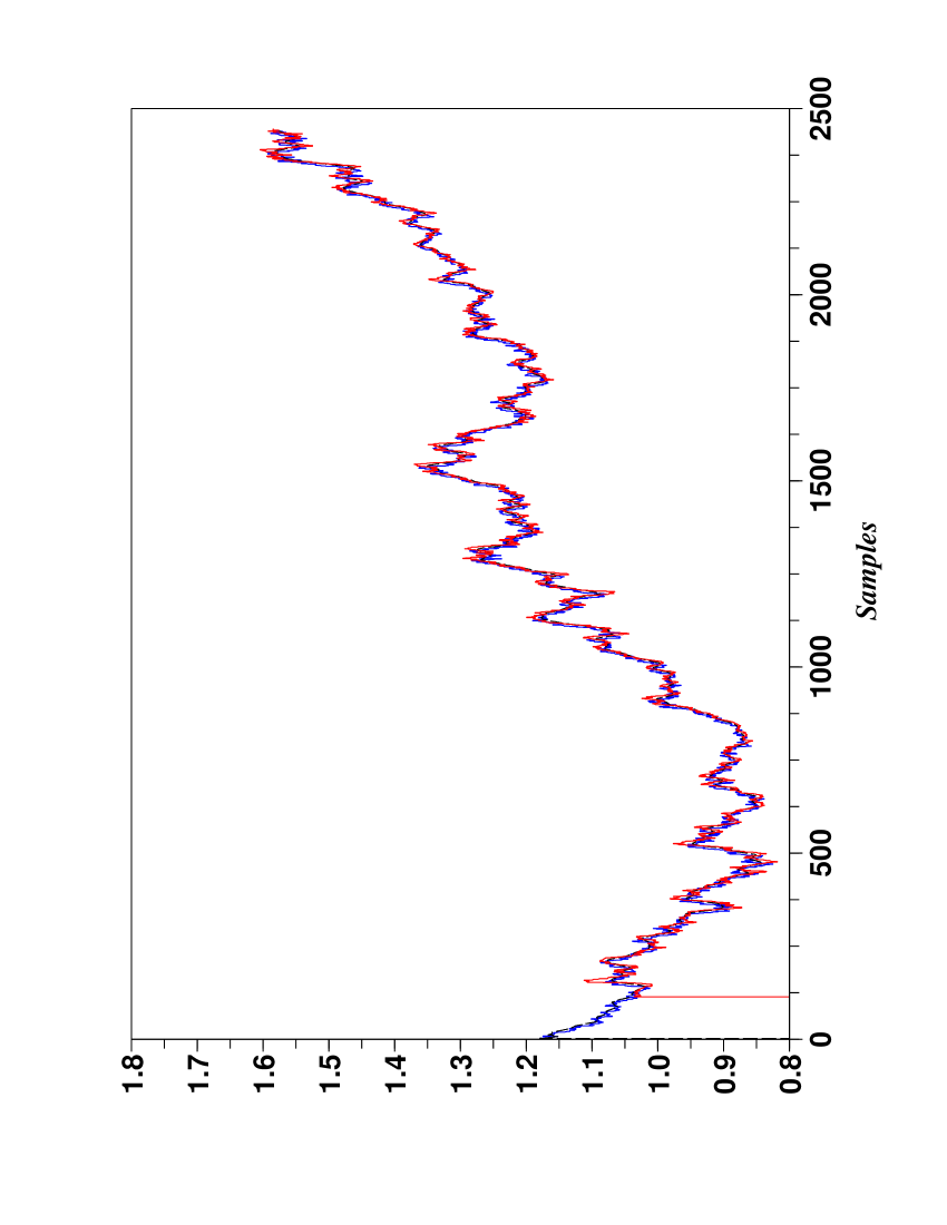
Figure 1: Exchange rates (blue –), filtered signal (black - -), forecasted signal ($5$ days ahead) (red –)

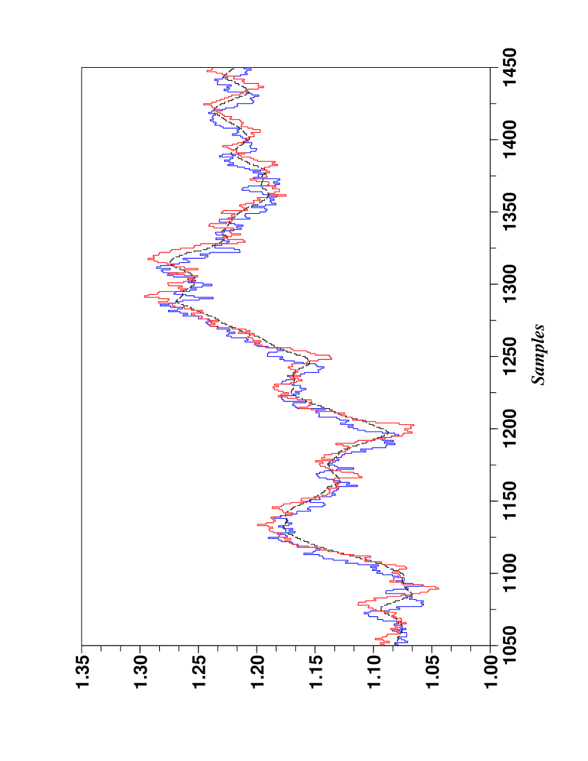
Figure 2: Zoom of Figure 1

3.1 Forecasting the trendline

In order to forecast the exchange rate $5$ days ahead we apply the rules sketched in Sect. 2.3 and we utilize a linear difference equation (1) of order $3$ (the filtered values of the exchange rates are given by the black lines in the Figures 1, 2). Fig. 3 provides the estimated values of the coefficients of the difference equation. The results on the forecasted values of the exchange rates are depicted by the red lines in the Figures 1 and 2, which should be viewed as a predicted trendline.

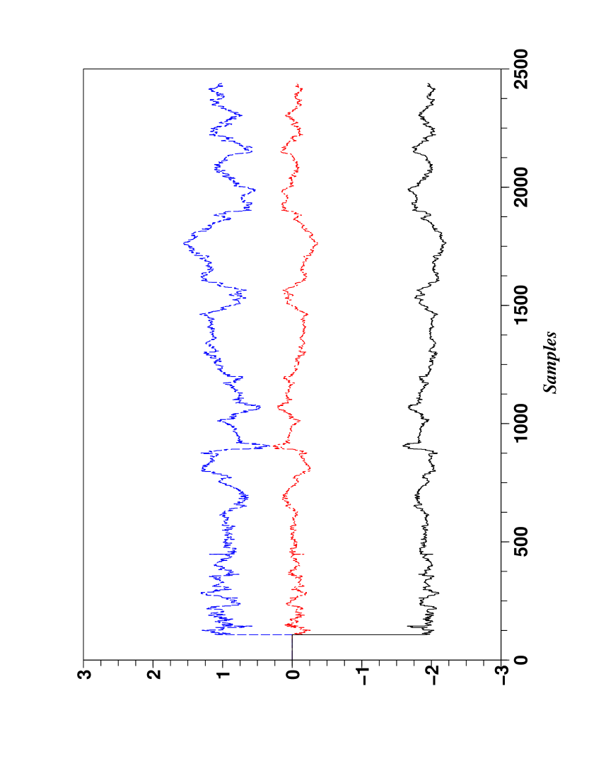
Figure 3: Parameter estimations $a_{1}$ (red $-.-$), $a_{2}$ (blue $--$) and $a_{3}$ (black $--$) ($5$ days ahead)

3.2 Above or under the predicted trendline?

Consider again the “error” $\nu(t)$ in Eq. (2) and its moving average $\text{MA}_{\nu,N}(t)$ in Eq. (6). Forecasting $\text{MA}_{\nu,N}(t)$ as in Sect. 3.1 tells us an expected position with respect to the forecasted trendline. The blue line of Fig. 4 displays the result for the window size $N=100$. The meaning of the indicators $\triangle$ and $\nabla$ is clear.

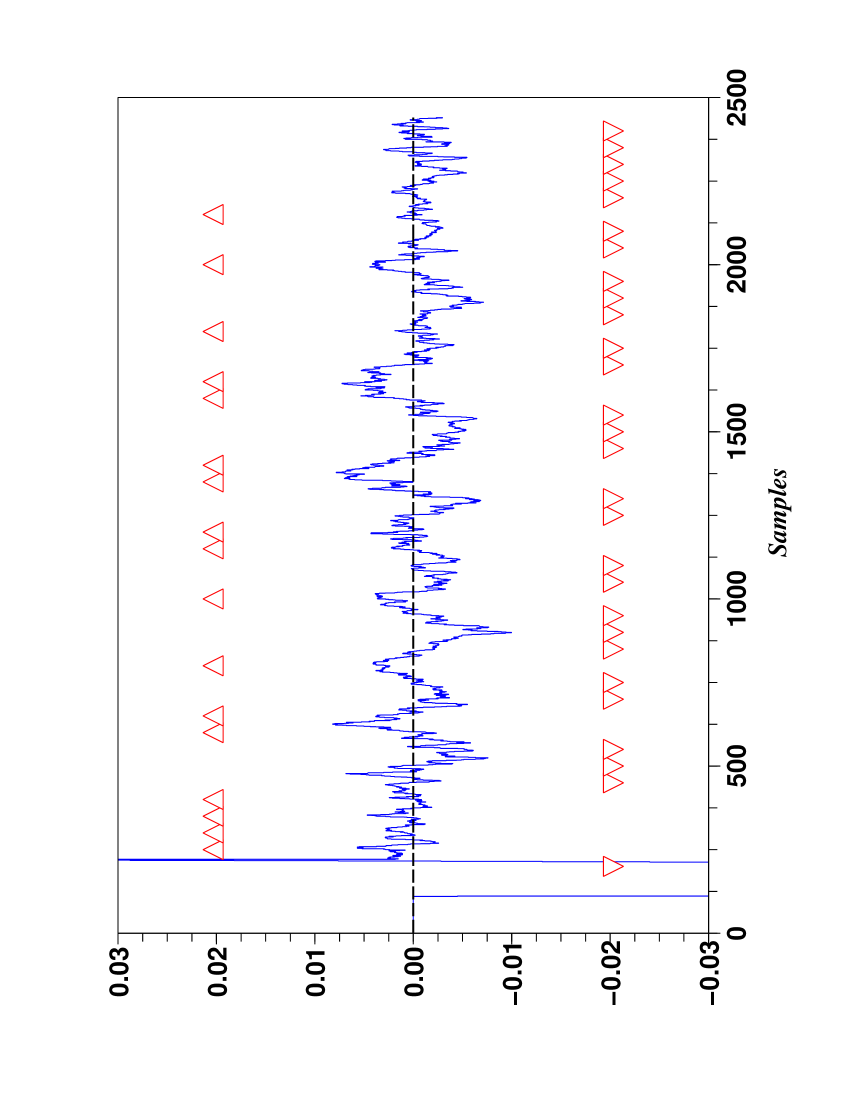
Figure 4: Predicted position w.r.t. the trendline ($5$ days ahead) – $\nabla$: above, $\triangle$: under

Table 1 compares for various window sizes the signs of the predicted values of $\text{MA}_{\nu,N}(t)$, which tells us if one should expect to be above or under the trendline, with the true positions of $x(t)$ with respect to the trendline. The results are expressed via percentages.

Window’s size	Percentage
$50$	$65.6\%$
$100$	$88.3\%$
$200$	$62.3\%$
$300$	$67.1\%$

Table 1: Comparison between the sign of the predicted value of $\text{MA}_{\nu,N}(t)$ and the true position of $x(t)$ w.r.t. the trendline ($5$ days ahead).

3.3 Predicted volatility w.r.t. the trendline

Introduce the moving standard deviation

$${\small\begin{array}[]{l}\text{MSTD}_{\nu,N}(t)=\\ \sqrt{\frac{\sum_{\tau=0}^{N}(\nu(t+\tau)-\text{MA}_{\nu,N}(t-N+\tau))^{2}}{N+1}}\end{array}}$$

and forecast it as in Sect. 3.2. The results, which are displayed for a window size $N=100$ in Table 2 and Fig. 5 via the familiar confidence intervals, confirm the time-dependence of the variance, i.e., the heteroscedasticity.

Confidence intervals	Prediction	Real
mean-$3\times$std,mean+$3\times$std	$99\%$	$98.7\%$
mean-$2\times$std,mean+$2\times$std	$95\%$	$92.2\%$
mean-std,mean+std	$68\%$	$64.4\%$

Table 2: Confidence interval validations ($5$ days ahead)

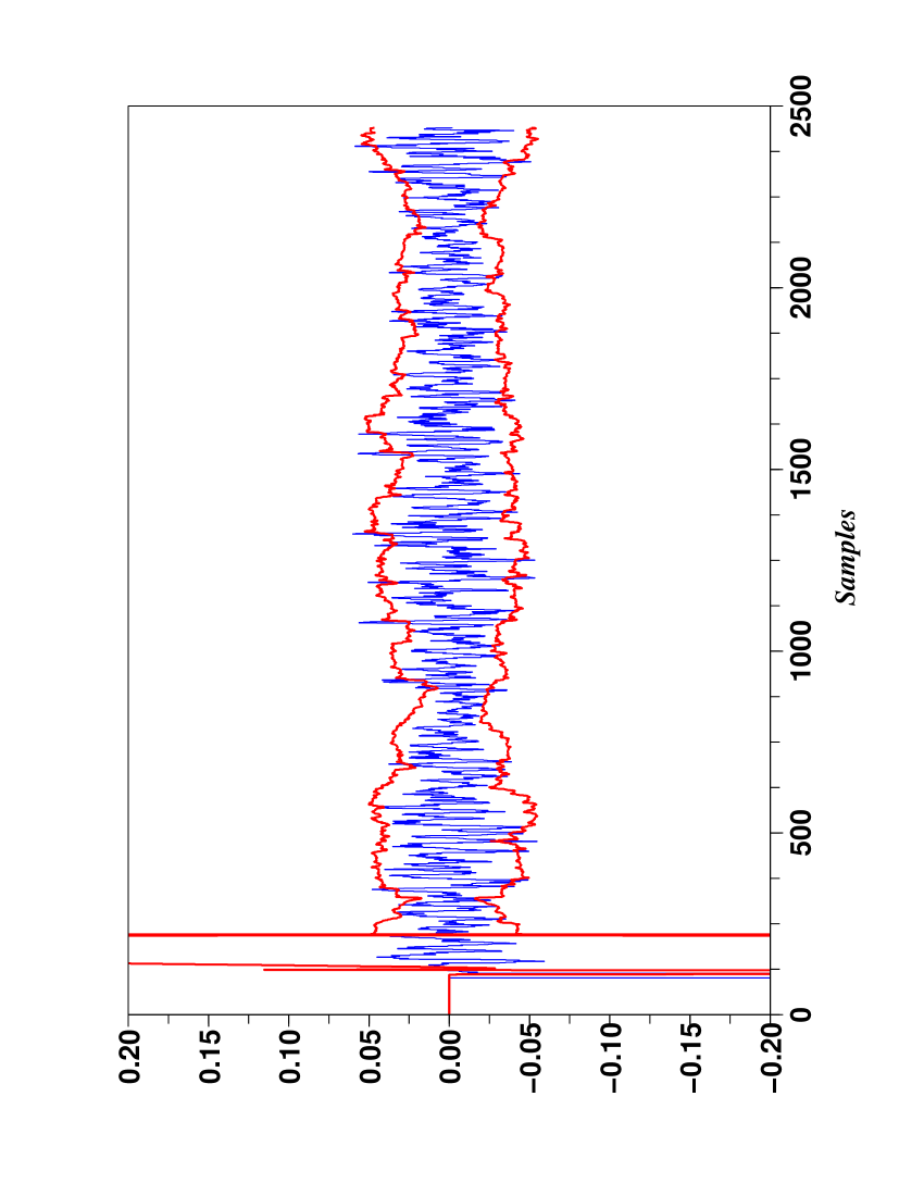
Figure 5: Confidence interval ($95\%$) ($5$ days ahead)

3.4 Forcasting 10 days ahead

Figures 6, 7, 8, 9 display the same type of results as in Sections 3.1, 3.2, 3.3 via similar computations for a forecasting $10$ days ahead. The quality of the computer simulations only slightly deteriorates.

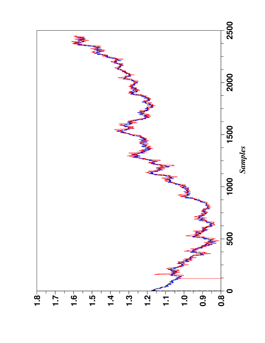
Figure 6: Exchange rates (blue –), filtered signal (black - -), forecasted signal (red –) ($10$ days ahead)

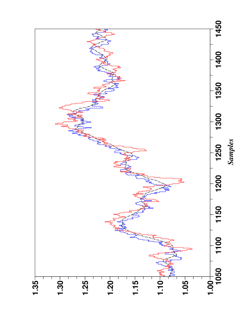
Figure 7: Zoom of Figure 6

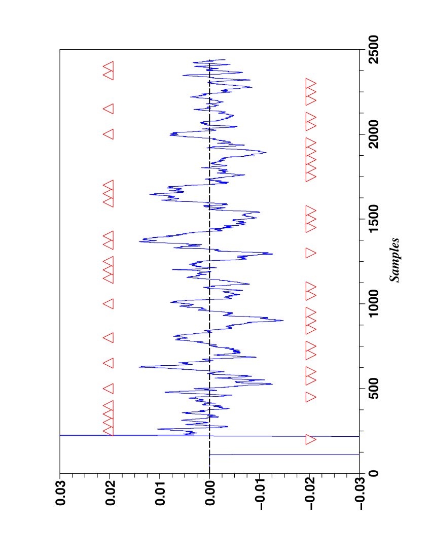
Figure 8: Predicted position w.r.t. the trendline ($10$ days ahead) – $\nabla$: above, $\triangle$: under

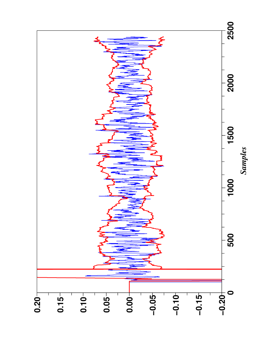
Figure 9: Confidence interval ($95\%$) ($10$ days ahead)

4 Conclusion

The existence of trends, which is

• the key assumption in technical analysis,

• quite foreign, to the best of our knowledge, to the academic mathematical finance, where the paradigm of random walks is prevalent (see, e.g., Wilmott (2006)),

is fundamental in our approach. A theoretical justification will appear soon Fliess & Join (2009). We hope it will lead to a sound foundation of technical analysis, which will bring as a byproduct easily implementable real-time computer programs.

Acknowledgement. The authors wish to thank G. Daval-Leclercq (Société Générale - Corporate & Investment Banking) for helpful discussions and comments.

References

- (1)
- Aronson (2007) Aronson D. (2007). Evidence-Based Technical Analysis. Wiley.
- Béchu, Bertrand & Nebenzahl (2008) Béchu T., Bertrand E., Nebenzahl J. (2008). L’analyse technique (6e éd.). Economica.
- Blanchet-Scalliet, Diop, Gibson, Talay & Tanré (2007) Blanchet-Scalliet C., Diop A., Gibson R., Talay D., Tanré E. (2007). Technical analysis compared to mathematical models based methods under parameters mis-specification. J. Banking Finance, 31, 1351–1373.
- Bouchaud & Potters (1997) Bouchaud J.-P., Potters M. (1997). Théorie des risques financiers. Eyrolles. English translation (2000): Theory of Financial Risks. Cambridge University Press.
- Box, Jenkins & Reinsel (1994) Box G.E.P., Jenkins G.M., Reinsel, G. (1994). Time Series Analysis: Forecasting and Control (3rd ed.). Prentice Hall.
- Chambert-Loir (2005) Chambert-Loir A. (2005). Algèbre corporelle. Édit. École Polytechnique. English translation (2005): A Field Guide to Algebra. Springer.
- Dacorogna, Gençay, Müller, Olsen & Pictet (2001) Dacorogna M.M., Gençay R., Müller U., Olsen R.B., Pictet O.V. (2001). An Introduction to High Frequency Finance. Academic Press.
- Doetsch (1967) Doetsch G. (1967). Funktionaltransformationen. In R. Sauer, L. Szabó (Eds): Mathematische Hilfsmittel des Ingenieurs, 1. Teil, pp. 232–484. Springer.
- Durlauf & Philips (1988) Durlauf S.N., Philips P.C.B. (1988). Trends versus random walks in time series analysis. Econometrica, 56, 1333–1354.
- Fliess (2008) Fliess M. (2008). Critique du rapport signal à bruit en communications numériques. ARIMA, to appear. Online http://hal.inria.fr/inria-00311719/en/.
- Fliess, Fuchshumer, Schöberl, Schlacher & Sira-Ramírez (2008) Fliess M., Fuchshumer S., Schöberl M., Schlacher K., Sira-Ramírez H. (2008). An introduction to algebraic discrete-time linear parametric identification with a concrete application. J. europ. syst. automat., 42, 211–232.
- Fliess & Join (2008) Fliess M., Join C. (2008). Commande sans modèle et commande à modèle restreint, e-STA, 5. Online http://hal.inria.fr/inria-00288107/en/.
- Fliess & Join (2009) Fliess M., Join C. (2009). A mathematical proof of the existence of trends in financial time series. Int. Conf. Systems Theory: Modelling, Analysis and Control. Fes, Marocco. Soon online http://hal.inria.fr/INRIA.
- Fliess, Join & Sira-Ramírez (2004) Fliess M., Join C., Sira-Ramírez H. (2004). Robust residual generation for linear fault diagnosis: an algebraic setting with examples. Int. J. Control, 77, 1223–1242.
- Fliess, Join & Sira-Ramírez (2008) Fliess M., Join C., Sira-Ramírez H. (2008). Non-linear estimation is easy. Int. J. Modelling Identification Control, 4, 12–27.
- Fliess & Sira-Ramírez (2003) Fliess M., Sira-Ramírez H. (2003). An algebraic framework for linear identification. ESAIM Control Optimiz. Calculus Variat., 9, 151–168.
- Fliess & Sira-Ramírez (2004) Fliess, M., Sira-Ramírez, H. (2004). Reconstructeurs d’état. C.R. Acad. Sci. Paris Ser. I, 338, 91–96.
- Fliess & Sira-Ramírez (2008) Fliess M., Sira-Ramírez H. (2008). Closed-loop parametric identification for continuous-time linear systems via new algebraic techniques. In H. Garnier, L. Wang (Eds): Identification of Continuous-time Models from Sampled Data, pp. 363–391, Springer.
- Gençay, Selçuk & Hafner (2002) Gençay R., Selçuk F., Whitcher B. (2002). An Introduction to Wavelets and Other Filtering Methods in Finance and Economics. Academic Press.
- Gouriéroux & Monfort (1995) Gouriéroux C., Monfort A. (1995). Séries temporelles et modèles dynamiques (2e éd.). Economica. English translation (1996): Time Series and Dynamic Models. Cambridge University Press.
- Hamilton (1994) Hamilton J.D. (1994). Time Series Analysis. Princeton University Press.
- Kaufman (2005) Kaufman P.J. (2005). New Trading Systems and Methods (4th ed.). Wiley.
- Jury (1964) Jury E.I. (1964). Theory and Application of the -Transform Method. Wiley.
- Kirkpatrick & Dahlquist (2006) Kirkpatrick C.D., Dahlquist J.R. (2006). Technical Analysis: The Complete Resource for Financial Market Technicians. FT Press.
- Lang (2002) Lang S. (2002). Algebra (3rd rev. ed.). Springer.
- Lo, Mamaysky & Wang (2000) Lo A.W., Mamaysky H., Wang J. (2000). Foundations of technical analysis: computational algorithms, statistical inference, and empirical implementation. J. Finance, 55, 1705-1765.
- Mandelbrot & Hudson (2004) Mandelbrot B.B., Hudson R.L. (2004). The (Mis) Behavior of Markets. Basic Books.
- Markovsky, Willems, van Huffel, de Moor & Pintelon (2005) Markovsky I., Willems J.C., van Huffel S., de Moor B., Pintelon R. (2005). Application of structured total least squares for system identification and model reduction. IEEE Trans. Automat. Control, 50, 1490-1500.
- Mboup, Join & Fliess (2008) Mboup M., Join C., Fliess M. (2008). A delay estimation approach to change-point detection. Proc. 16th Medit. Conf. Control Automation, Ajaccio. Online http://hal.inria.fr/inria-00179775/en/.
- Mboup, Join & Fliess (2009) Mboup M., Join C., Fliess M. (2009). Numerical differentiation with annihilators in noisy environment. Numer. Algor., DOI: 10.1007/s11075-008-9236-1.
- Murphy (1999) Murphy J.J. (1999). Technical Analysis of the Financial Markets (3rd rev. ed.). New York Institute of Finance.
- Paulos (2003) Paulos J.A. (2003). A Mathematician Plays the Stock Market. Basic Books.
- Sornette (2003) Sornette D. (2003). Why Stock Markets Crash: Critical Events in Complex Financial Systems. Princeton University Press.
- Taleb (1997) Taleb N. (1997). Dynamic Hedging. Wiley.
- Wilmott (2006) Wilmott P. (2006). Paul Wilmott on Quantitative Finance (2nd ed., 3 volumes). Wiley.