.
Photogalvanic effect and photoconductance in a quantum channel with a single short-range scatterer
Abstract
The influence of electromagnetic radiation on the electron transport in a quantum channel with a single short-range scatterer is investigated using a generalized Landauer-Büttiker approach. We have shown that asymmetrical position of the scatterer leads to appearance of the direct photocurrent in the system. The dependence of the photocurrent on the electron chemical potential, the position of the scatterer, and the frequency of the radiation is studied. We have shown that the photocurrent and the photoconductance oscillate as functions of the electron chemical potential. The nature of oscillations is discussed.
pacs:
73.23.Ad, 78.67.LtI Introduction
The study of electron transport in nanostructures under the external electromagnetic radiation has been attracting considerable attention during the last few years. The interest to the problem is stipulated by recent attempts to create a sensitive nanometer-size photodetector. Kos02 ; Kos03 ; Rao05 ; Row06 ; Ejr07 Photon-induced electron transport in a number of interesting systems such as quantum point contacts, Wyss93 ; Wyss95 ; Wir02 ; Kos02 field-effect transistors, Kos03 ; Row06 quantum dots, Rao05 and carbon nanotubes Mul04 ; Cho07 was studied in various experiments. Quantum ratchet effects induced by terahertz radiation were observed in GaN-based two-dimensional structures. Web08 Impurity photocurrent spectra of bulk GaAs and GaAs quantum wells doped with shallow donors were studied. Ale07 It was shown experimentally Wyss93 that the photoconductance of the quantum point contact oscillates with the gate voltage. In the case of asymmetrical illumination, the direct photocurrent arises in the quantum point contact. Wyss95 . The photocurrent was attributed to the radiation-induced thermopower.
A lot of theoretical models have been used to study the microwave induced electron transport in bulk materials and low-dimensional systems. Photon-assisted tunneling in a resonant double barrier system was investigated within the scattering approach. Ped98 Various quantum dot photodetectors Lim06 ; Apa07 ; Vil07 were studied theoretically. The photoconductivity of quantum wires and microconstrictions with an adiabatic geometry was investigated using different calculation methods. Gri95 ; Maa96 ; Bor97 ; Blo98 ; Gal04 It was found that absorbtion of high-frequency electromagnetic field polarized in transversal direction results in oscillations of the photoconductance as a function of the gate voltage. Circular photogalvanic effect in bent Per05 and helical Mag03 one-dimensional quantum wires was studied. Radiation-induced current in quantum wires with side-coupled nanorings was calculated. Per07 One-dimensional quantum pump based on two harmonically oscillating -potentials was investigated in Refs. Bra05, ; Mah08, . Various interesting photon and phonon depended effects were predicted in carbon nanotube devices. Kib05 ; Kib95 ; Kib01 ; Ste04 A number of papers are devoted to the theoretical study of the spin-depended photogalvanic effects. Gan02 ; Gan07 ; Tar05 ; TI05 ; Gla05 ; Ivc04 ; Fed05 ; Ivc02
A consistent quantitative theory of photogalvanic effect in bulk samples was given by Belinicher and Sturman. Bel80 The necessary condition for appearance of the photocurrent is the absence of the inversion symmetry in the system. In the macroscopic samples, the absence may be stipulated by the asymmetry of the lattice Web08 ; Bel80 or by oriented asymmetric scatterers. Ent06 ; Che08
Ballistic transport regime in quasi one-dimensional nanostructueres allows another mechanism. The symmetry may be broken by an asymmetrically located single scatterer, for instance, a potential barrier Tag99 or an impurity. In the present paper, we consider one of the simplest nanoscale system that allows generation of the direct current induced by electromagnetical radiation.
II Hamiltonian
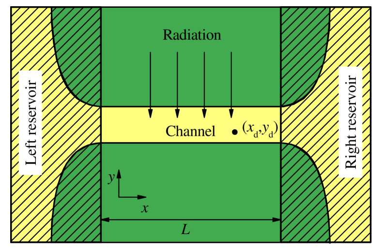
The purpose of the present paper is the theoretical investigation of the photocurrent in a quantum channel containing a single point defect. It should be mentioned that the elastic scattering in similar systems has been widely discussed in literature. Yac90 ; Lev91 ; Lev92 ; Gur93 ; Lub93 ; Suk94 ; Gei93 We consider the channel that is formed in the two-dimensional electron gas by parabolic confining potential. The schematic view of the device is shown in Fig. 1.
The electron motion in the channel is described by the Hamiltonian
| (1) |
where is effective electron mass, is the frequency of parabolic confining potential, and are projections of the momentum (the direction corresponds to the axis of the channel). Eigenvalues and eigenfunctions of the Hamiltonian are well-known
| (2) |
where , and are oscillator functions. We note that the effective channel width is determined by the number of occupied subbands and by the characteristic oscillator length .
The short-range defect is modelled by the zero-range potential, Dem88 ; Alb88 ; Bru03 ; Gey03 ; Gei93 and therefore the Hamiltonian of the channel with the defect is a point perturbation of the Hamiltonian . Actually, the point perturbation is determined by boundary conditions for the wave function at the defect point. The similar method has been used earlier Gey03 ; MP05 ; MP07 for modelling of point contacts.
Boundary values for the wave function are determined with the help of the zero-range potential theory. Dem88 ; Alb88 ; Bru03 ; Gey03 The theory shows that the electron wave function has the logarithmic singularity in a vicinity of the defect point . As follows form the theory of zero-range potentials the wave function of the Hamiltonian with the point perturbation may be represented in terms of the Green’s function. That is why the wave function has the same singularity as the Green’s function in the vicinity the point of perturbation. We note that the form of the singularity is determined by the dimension of space only. It is independent on energy and form of smooth confining potential. In particular, the singularity is logarithmic in the two-dimensional case
| (3) |
where and are complex coefficients, and is the remainder term that tends to zero in the limit . Coefficients and play the role of boundary values for the wave function . They are independent of . The boundary conditions at the point of contact are some linear relations between and :
| (4) |
Here the coefficient determines the strength of the zero-range potential at the point . It should be noted that the zero-range potential is attractive and the limit corresponds to the absence of the point perturbation.
We suppose that the channel is exposed by an external electromagnetic wave propagating in the direction and polarized in the direction. We assume that electron-photon interaction takes place in the region of the channel only that may be realized by an antenna Wyss93 or by an opaque diaphragm (Fig. 1). In the view of these assumptions the influence of the electromagnetic field on the electron is described by the operator
| (5) | |||||
where is the amplitude of the electric field, is the frequency of radiation, and is the Heaviside step function, i.e., for and otherwise.
To obtain the electric current in the channel we use the generalization Dat92 ; Maa96 ; Per05 ; Per07 ; Maa97 of the Landauer–Büttiker formula Lan57 ; But86 that takes into account the radiation
| (6) | |||||
Here is the transmission probability between the state with the energy and the quantum number in the left reservoir and the state with the energy and the quantum number in the right reservoir, and are Fermi distribution functions for the left and the right reservoirs respectively, and is the number of absorbed photons (negative corresponds to emission of photons). Function (here means left (L) or right (R) electron reservoir) has the form
| (7) |
where is the chemical potential in the -th reservoir and is temperature. In the paper, we consider the first order of the perturbation theory and restrict ourselves to .
Transmission coefficients can be represented via transmission amplitudes (here indexes and mean left () or right () reservoir)
| (8) |
where wave number is given by
| (9) |
III Photocurrent
In the linear response approximation the current is represented in the form
| (10) |
where is the zero-bias photocurrent, is conductance of the system, and is the bias voltage. The photocurrent is given by
| (11) |
where
| (12) | |||||
We note that the terms with are cancelled in Eq. (12) due to the time-reversal symmetry of elastic scattering.
To obtain the transmission probabilities we use the concept of quasi-energy states. Zel73 Since the Hamiltonian of the system varies periodically with time the electron wave function may be represented in the form
| (13) |
where is the quasi-energy. From the Schrödinger equation, we obtain the following relations for the functions
In the first order of the perturbation theory, we restrict ourselves to and express the functions in terms of the Green’s function of the Hamiltonian
| (14) |
where is determined from the equation
| (15) |
It should be mentioned that the Green’s function is the integral kernel of the operator .
We note, that at real quasi-energies the perturbation theory is inapplicable in the vicinity of the eigenvalues of the Hamiltonian since the Green’s function has the root singularities at these energies. This phenomenon is stipulated by infinite lifetime of the states with zero speed. Therefore the electrons having zero speed are influenced by electromagnetic field for an infinitely long period of time, and hence the transition probability for these electrons is not small. To avoid peculiarities in the expression for we introduce the complex quasi-energy . The imaginary part of the quasi-energy is a phenomenological parameter that may be expressed in terms of effective state lifetime via the relation . We mention that broadening may be caused by spontaneous transitions and inelastic scattering processes.
The zero-range potentials theory Alb88 ; Gey03 shows that the eigenfunction of the Hamiltonian can be represented in the form
| (16) |
where is the eigenfunction and is the Green’s function of the Hamiltonian , is a parameter that determines the strength of the point perturbation, and is the Krein’s Q-function that is the renormalized Green’s function. The renormalization is obtained by subtracting of the logarithmic singularity at from . We note, that Krein’s Q-function is defined up to additive constant. This constant determines the connection between the value of parameter and the strength of point perturbation. In the present paper, we focus on effects independent of the value of the point potential, so the value of constant is not very important for our purposes. Since the form of singularity of the Green’s function is independent of energy we can get Krein’s Q-function by the following equation Gei93
| (17) |
Here is some fixed value of energy that is smaller than the ground state energy. Actually, determines the difference between parameters from Eq. (16) and from Eq. (4). In the present paper, we take and define the strength of the point perturbation by the parameter .
To obtain the transmission amplitudes we should take as an incident wave propagating in the mode
| (18) |
The Green’s function is given by equation
| (19) |
where and .
The Green’s function of the Hamiltonian is represented in terms of the Green’s function of the Hamiltonian using the Krein resolvent formula Alb88 ; Bru03
| (20) |
From the asymptotics of the functions at the right edge of the channel we obtain transmission amplitudes and . Details of the derivation are given in the Appendix. Then we calculate transmission coefficients and the photocurrent using Eq. (11).
To write down the equation for we need some preliminary notations:
and
Now we can represent the amplitude in the form
| (21) |
where
| (22) | |||
| (23) | |||
| (24) | |||
| (25) |
Here , and are elementary integrals:
The transmission amplitude from the right to the left reservoir is obtained from Eq. (21) via replacing by in integrals and .

The dependence of the photocurrent on the chemical potential is represented in Fig. 2(a). The corresponding values of are shown in Fig. 2(b). One can see that photocurrent oscillates with increase of the chemical potential. The amplitude of oscillations depends linearly on the intensity of radiation. The contribution to the photocurrent has sharp peaks in the vicinity of the energies . The sign of contribution is different for even and odd values of .
To explain the behavior of the photocurrent we consider a simplified model of the system. In this model, the channel is divided into three parts and the transmission probabilities through each part are combined incoherently. That means the transmission coefficients are defined by equation
| (26) |
where and are photon assisted transition probabilities in the left and the right parts of the channel and are elastic transmission coefficients without taking the radiation into account. The transition probabilities are determined by the same quasi-energy approach as indicated above but Eqs. (18) and (19) are used for the wave function and the Green’s function instead of Eqs. (16) and (20):
| (27) | |||||
Here for the left part of the channel and for the right part.
The transmission coefficients are obtained from Eq. (16) and have the form
| (28) |
Although the approach is sufficiently rough it allows to obtain a simple explanation of the phenomena. According to this approach the photocurrent is stipulated by the difference in transmission probabilities for states with different quantum number . Using the symmetric properties of transmission coefficient we can represent the difference in the form
| (29) | |||||
where and is total transmission probability for mode
| (30) |
One can see that the electron transition contributes positively to the photocurrent if the transmission probability increases and contributes negatively in the opposite case.
If the scatterer is located on the axis of the channel () then the states with odd are not reflected since the wave function vanishes at the point . Hence the electron transitions from the state with even to the state with odd increase the transmission probability. The number of occupied states of different parity depends on the chemical potential. Therefore the photocurrent oscillates with increase of the chemical potential.
Let us consider the simplest case of the axial scatterer position (), and resonance frequency of radiation (). If the defect is placed in the vicinity of the channel center (), our approach gives the following asymptotic equation for the difference of transmission coefficients:
| (31) |
as . Here . One can see from Eq. (31) that the contribution to the photocurrent from the vicinity of is positive for even and negative for odd . The photocurrent is proportional to and it vanishes in the case of symmetrical disposition of the defect. The amplitude of the peak grows with increase of the mode number proportional to . Therefore the amplitude of the photocurrent oscillations increases with chemical potential. As it follows from Eq. (31), the contribution to the photocurrent is maximal from slow electrons. This result is in agreement with Fig. 2(b) based on the more precise approach. The phenomenon is caused by sufficiently long exposure time and large density of states for slow electrons.
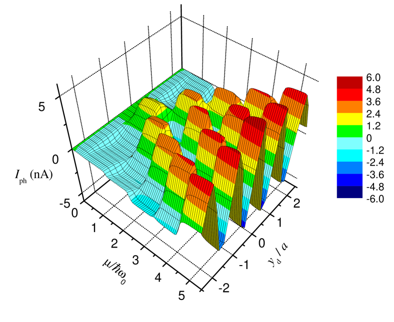
Let us discuss the effect of the scatterer position. The dependence of the photocurrent on the chemical potential and the scatterer position is represented in Fig. 3. One can see that the sequence of peaks and dips of the photocurrent is changed if the scatterer is shifted from the channel axis (). The photocurrent tends to zero when the defect is placed sufficiently far from the channel axis () because the defect does not change the transmission probability in this case.
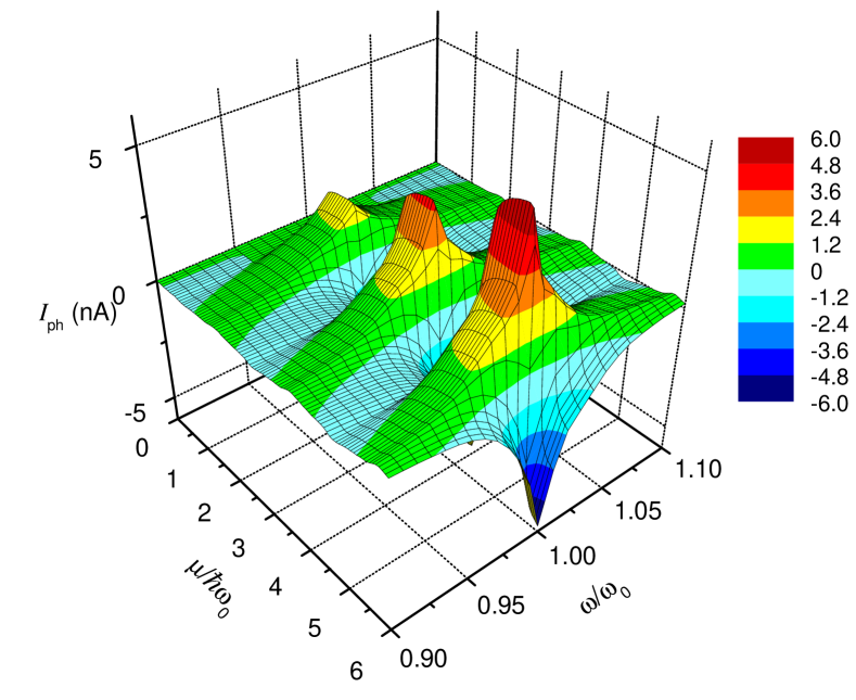
The dependence of the photocurrent on the frequency of radiation and the chemical potential is represented in Fig. 4. One can see that the photocurrent decreases with deviation of the frequency from the resonance value .
Our numerical analysis shows that more simplified ’incoherent’ method of calculation is in qualitatively agreement with more precise method based on Eqs. (21)-(25). But asymptotics given by Eq. (31) for is not valid for very small values of . According to Eq. (31) at as . However, more precise analysis based on Eqs. (21)-(25) shows that remains finite. The difference between the approaches is based on taking the quantum coherence into account. We mention, that all figures are plotted using Eqs. (21)-(25).
IV Photoconductance
Let us consider the effect of the radiation on the conductive properties of the device. According to Eqs. (6) and (10) the conductance can be represented in the form
| (32) |
where is the conductance quantum and is given by
| (33) | |||||
It should be noted that contains contributions from elastic and inelastic processes for and respectively. Hence to obtain the photoconductance we have to find the modification of the transmission coefficients that corresponds to electron motion without absorbtion or emission of photons. These coefficients could not be found from the first-order perturbation theory since the corrections for the transmission amplitudes should be the second-order terms. Therefore, to find the corrections we use the current conservation law
| (34) |
where are reflection coefficients. Similar relation is valid for electrons travelling from the right to the left reservoir. We mention that the coefficients were cancelled in Eq. (11) due to the time reversal symmetry.
Using Eq. (34), we represent in the form
| (35) |
where is ’dark’ quasiballistic conductance of the channel with the defect and is photoconductance.
At the zero temperature the conductance may be represented in the form
| (36) |
where are transmission coefficients for elastic scattering given by Eq. (28).
Using Eqs. (19) and (28), we can represent the zero-temperature conductance in the form
| (37) |
Here is the number of occupied subbands ( means integer part of ). It is clear, that at finite temperatures the conductance is given by the integral similar to Eq. (32). The dependence in the case of axial scatterer position () is shown in Fig. 5. One can see that the steps corresponding to even values of are smoothed due to scattering on the defect while the steps with odd values of are conserved because electrons with odd values of are not scattered.

Photoconductance is given by equation
| (38) |
where
| (39) |
Here and are total elastic transmission and reflection probabilities for mode while and are total photon-assisted transmission and reflection probabilities for mode . Probability is given by Eq. (30) and is defined by . According to Eq. (34), and are given by the following equations:
| (40) | |||||
and
| (41) | |||||
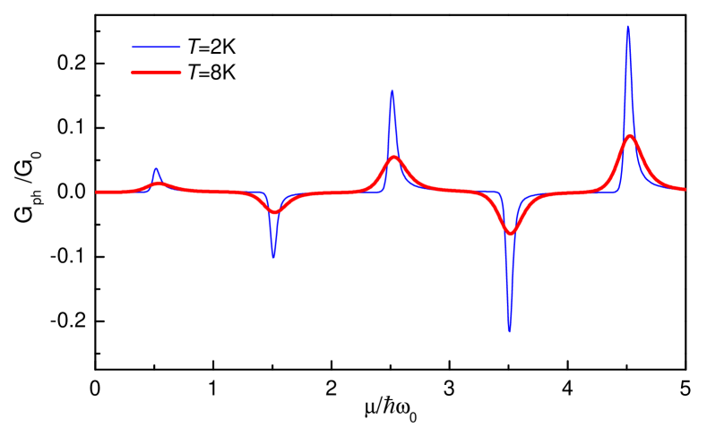
The photoconductance as a function of the chemical potential oscillates as well as the photocurrent. The dependence is shown in Fig. 6. One can see from Eq. (38) that the dependence contains the derivative of the Fermi function in contrast to the dependence , therefore peaks and dips of the photoconductance are sharper and more sensitive to the growth of the temperature. The increase of temperature leads to smoothing of peaks and decrease of their amplitudes. The amplitude of the photoconductance peaks is proportional to intensity of radiation. If the defect is placed in the central cross-section of the channel then the photoconductance is proportional to squared length of the channel.
V Conclusion
Photon-induced electron transport in the quantum channel with a single point defect is investigated using modified Landauer–Büttiker formalism. The dependence of the photocurrent on the electron chemical potential is studied both analytically and numerically. We have shown that the photocurrent is stipulated by different transmission probabilities for different electron subbands in the channel. If the defect is placed on the axis of the channel then the odd electron subbands are not reflected by the defect since corresponding wave function vanishes at the point of the scatterer. Thus the photon-induced transitions between electron subbands of different parity can either increase or decrease the transmission probability. The probability of photon-induced transition depends on the distance from the channel edge to the defect. Therefore, the direct current arises in the case of asymmetric scatterer position. We have shown that the photocurrent oscillates as a function of chemical potential. The direction of the current is determined by the number of occupied subbands of different parity. The sequence of oscillating minima and maxima is changed if the scatterer is placed aside the channel axis. The photocurrent is proportional to the intensity of radiation and grows with increase of the lifetime . The amplitude of oscillations reaches maximum when the frequency of radiation coincides with the characteristic frequency of the confining potential in the channel. This feature of the system gives the possibility to vary the resonance frequency by changing the geometry of the channel.
If the scatterer is placed in the central cross-section of the channel the photocurrent is absent but the defect influences the conductance of the system. The total conductance of the system may be represented as a sum of the ’dark’ quasiballistic conductance and the photoconductance that is proportional to the intensity of radiation. The dependence of the photoconductance on the chemical potential contains sharp peaks and dips in the vicinity of steps of the ballistic conductance. In the case of axial defect position, the sign of the photoconductance is determined by the parity of the highest occupied subband in the channel at the zero temperature. The nature of the photoconductance oscillations is similar to the nature of the photocurrent oscillations. However, the dependence of the photoconductance on the chemical potential is sharper and more sensitive to the temperature than the dependence of the photocurrent. The grows of temperature leads to the smoothing of photoconductance peaks and decrease of their amplitudes.
ACKNOWLEDGEMENTS
The authors are grateful to V. A. Margulis for helpful discussions. The work has been supported by Grant of the President of the Russian Federation for young scientists (grant MK-4480.2007.2) and by Russian Foundation for Basic Research (grant 08-02-01035).
APPENDIX
To obtain the transmission amplitude from the left to the right reservoir we have to compare the asymptotics of the wave function at the left and the right edge of the channel. The wave function is given by Eq. (14). We take the incident wave from the left reservoir in the form Eq. (18). Using Eq. (16) for and Eq. (20) for we may represent the function as a sum of four terms
| (42) |
where functions are given by
| (43) |
| (44) |
| (45) |
| (46) |
Taken into consideration properties of oscillator functions we have
| (47) |
Using Eqs. (18), (19), and (47) we obtain
| (48) |
| (49) |
Now we substitute Eqs. (48) and (49) into Eqs. (43)–(46) and perform the integration over . One can see that integration over includes only finite interval due to the -functions. Integration over may be performed easily due to the orthogonality of the oscillator functions . For example, integration in equation (43) gives for
| (50) |
Then we obtain the following form for functions at the right edge of the channel ()
| (51) |
where coefficients are given by Eqs. (22)–(25). It should be mentioned that we have to take into account the exponential factor in the transmission amplitude since we deal with complex quasienergies and consequently complex wave numbers . This factor does not vanish during the current calculation hence it should be conserved in the equation for transmission amplitude.
To get the transmission amplitude from the right to the left reservoir we need do consider incident wave that is injected from the right edge of the channel and propagate to the left edge. One can see that the computation remains the same if we invert the direction of the axis. Therefore the final expressions for transmission amplitude may be obtained from Eqs. (22)–(25) by replacement of with .
References
- (1) H. Kosaka, D. S. Rao, H. D. Robinson, P. Bandaru, K. Makita, and E. Yablonovitch Phys. Rev. B 67, 045104 (2003).
- (2) M. A. Rowe, E. J. Gansen, M. Greene, R. H. Hadfield, T. E. Harvey, M. Y. Su, S. W. Nam, R. P. Mirin, and D. Rosenberg, Appl. Phys. Lett. 89, 253505 (2006).
- (3) D. S. Rao, T. Szkopek, H. D. Robinson, E. Yablonovitch, and H.-W. Jiang, J. Appl. Phys. 98, 114507 (2005)
- (4) M. Ejrnaes, R. Cristiano, A. Gaggero, F. Mattioli, R. Leoni, B. Voronov, and G. Gol’tsman, Appl. Phys. Lett. 91, 262509 (2007).
- (5) H. Kosaka, D. S. Rao, H. D. Robinson, P. Bandaru, T. Sakamoto, and E. Yablonovitch, Phys. Rev. B 65, 201307(R) (2002).
- (6) R. A. Wyss, C. C. Eugster, J. A. del Alamo, and Q. Hu, Appl. Phys. Lett. 62, 1522 (1993).
- (7) R. A. Wyss, C. C. Eugster, J. A. del Alamo, Q. Hu, M. J. Rooks, and M. R. Melloch, Appl. Phys. Lett. 66, 1144 (1995).
- (8) R. Wirtz, R. Newbury, J. T. Nicholls, W. R. Tribe, M. Y. Simmons, and M. Pepper, Phys. Rev. B 65, 233316 (2002).
- (9) E. Mulazzi, R. Perego, H. Aarab, L. Mihut, S. Lefrant, E. Faulques, and J. Wéry, Phys. Rev. B 70, 155206 (2004).
- (10) D. Chowdhary and N. A. Kouklin, Phys. Rev. B 76, 035416 (2007).
- (11) W. Weber, L. E. Golub, S. N. Danilov, J. Karch, C. Reitmaier, B. Wittmann, V. V. Bel’kov, E. L. Ivchenko, Z. D. Kvon, N. Q. Vinh, A. F. G. van der Meer, B. Murdin, and S. D. Ganichev, Phys. Rev. B 77, 245304 (2008).
- (12) V. Ya. Aleshkin, A. V. Antonov, L. V. Gavrilenko, and V. I. Gavrilenko, Phys. Rev. B 75, 125201 (2007)
- (13) M. H. Pedersen and M. Büttiker, Phys. Rev. B 58, 12993 (1998).
- (14) H. Lim, B. Movaghar, S. Tsao, M. Taguchi, W. Zhang, A. A. Quivy, and M. Razeghi, Phys. Rev. B 74, 205321 (2006).
- (15) V. M. Apalkov, Phys. Rev. B 75, 035339 (2007).
- (16) J. M. Villas-Bôas, S. E. Ulloa, and A. O. Govorov, Phys. Rev. B 75, 155334 (2007).
- (17) A. Grincwajg, L. Y. Gorelik, V.Z. Kleiner, and R. I. Shekhter, Phys. Rev. B 52, 12168 (1995).
- (18) F. A. Maaø and L. Y. Gorelik, Phys. Rev. B 53, 15885 (1996).
- (19) V. S. Borovikov, L. Yu. Gorelik, V. Z. Kleĭner, and R. I. Shekhter, Fiz. Nizk. Temp. 23, 313 (1997) [Low. Temp. Phys. 23 230 (1997)].
- (20) S. Blom, L. Y. Gorelik, M. Jonson, R. I. Shekhter, A. G. Scherbakov, E. N. Bogachek, and U. Landman, Phys. Rev. B 58, 16305 (1998).
- (21) N. G. Galkin, V. A. Margulis, and A. V. Shorokhov, Phys. Rev. B 69, 113312 (2004).
- (22) Y. V. Pershin and C. Piermarocchi, Phys. Rev. B 72, 245331 (2005).
- (23) L. I. Magarill and M. V. Entin, Pis’ma Zh. Eksp. Teor. Fiz. 78, 249 (2003) [JETP Lett. 78, 213 (2003)].
- (24) Y. V. Pershin and C. Piermarocchi, Phys. Rev. B 75, 035326 (2007).
- (25) L. S. Braginski, M. M. Makhmudian, and M. V. Entin, Zh. Eksp. Teor. Fiz. 127, 1046 (2005) [JETP 100, 920 (2005)].
- (26) M.M. Mahmoodian, M.V. Entin, and L.S. Braginsky, Physica E (Amsterdam) 40 (5), 1205 (2008).
- (27) O. V. Kibis and M. E. Portnoi, Pis’ma Zh. Tekh. Fiz. 31, No. 15, 85 (2005) [Tech. Phys. Lett. 31, No. 8, 671 (2005)].
- (28) Kibis O. V., Romanov D. A. Fiz. Tverd. Tela (S.-Petersburg) 37, 127 (1995) [Phys. Solid State 37, 69 (1995)].
- (29) Kibis O. V. Fiz. Tverd. Tela (S.-Petersburg) 43, 2255 (2001) [Phys. Solid State 43, 2336 (2001)].
- (30) D. A. Stewart and F. Leonard, Phys. Rev. Lett. 93, 107401 (2004).
- (31) S. D. Ganichev, E. L. Ivchenko, V. V. Bel’kov, S. A. Tarasenko, M. Sollinger, D. Weiss, W. Wegscheider, and W. Prettl, Nature 417, 153 (2002).
- (32) S. D. Ganichev, S. N. Danilov, V. V. Bel’kov, S. Giglberger, S. A. Tarasenko, E. L. Ivchenko, D. Weiss, W. Jantsch, F. Schäffler, D. Gruber, and W. Prettl, Phys. Rev. B 75, 155317 (2007).
- (33) S. A. Tarasenko, Phys. Rev. B 72, 113302 (2005).
- (34) M. M. Glazov, P. S. Alekseev, M. A. Odnoblyudov, V. M. Chistyakov, S. A. Tarasenko, and I. N. Yassievich, Phys. Rev. B 71, 155313 (2005).
- (35) E. L. Ivchenko and S. A. Tarasenko, Zh. Eksp. Teor. Fiz. 126, 426 (2004) [JETP, 99, 379 (2004)].
- (36) S. A. Tarasenko and E. L. Ivchenko, Pis’ma Zh. Eksp. Teor. Fiz. 81, 292 (2005) [JETP Lett., 81, 231 (2005)].
- (37) E. L. Ivchenko, Phys. Usp. 45 1299 (2002).
- (38) A. Fedorov, Y. V. Pershin and C. Piermarocchi, Phys. Rev. B 72, 245327 (2005).
- (39) V. I. Belinicher and B. I. Sturman, Usp. Fiz. Nauk 130, 415 (1980) [Sov. Phys. Uspekhi 23, 199 (1980)].
- (40) M. V. Entin and L. I. Magarill, Phys. Rev. B 73, 205206 (2006).
- (41) A. D. Chepelianskii, M. V. Entin, L. I. Magarill, and D. L. Shepelyansky, Physica E (Amsterdam) 40, 1264 (2008).
- (42) O. Tageman and A. P. Singh, Phys. Rev. B 60, 15937 (1999).
- (43) A. Yacoby and Y. Imry, Phys. Rev. B 41, 5341 (1990).
- (44) Y. B. Levinson, M. I. Lubin, and E. V. Sukhorukov, Pis’ma Zh. Eksp. Teor. Fiz. 54, 405 (1991) [JETP Lett. 54, 401 (1991)].
- (45) Y. B. Levinson, M. I. Lubin, and E. V. Sukhorukov, Phys. Rev. B 45, 11936 (1992).
- (46) S. A. Gurvitz and Y. B. Levinson, Phys. Rev. B 47, 10578 (1993).
- (47) M. I. Lubin, Pis’ma Zh. Eksp. Teor. Fiz. 57, 346 (1993) [JETP Lett. 57, 361 (1993)].
- (48) E. V. Sukhorukov, M. I. Lubin, C. Kunze and Y. Levinson, Phys. Rev. B 49, 17191 (1994).
- (49) V.A. Geĭler, V.A. Margulis, and I.I. Chuchaev, Pis’ma Zh. Eksp. Teor. Fiz. 58, 668 (1993) [JETP Lett. 58, 648 (1993)].
- (50) Y. N. Demkov and V. N. Ostrovsky, Zero-Range Potentials and Their Applications in Atomic Physics (Plenum, New York, 1988).
- (51) S. Albeverio, F. Gesztesy, R. Höegh-Krohn, and H. Holden, Solvable Models in Quantum Mechanics (Springer-Verlag, Berlin, 1988).
- (52) J. Brüning and V. A. Geyler, J. Math. Phys. 44, 371 (2003).
- (53) V. A. Geyler, V. A. Margulis, and M. A. Pyataev, Zh. Eksp. Teor. Fiz. 124 851 (2003) [JETP 97, 763 (2003)].
- (54) V. A. Margulis and M. A. Pyataev, Phys. Rev. B 72, 075312 (2005).
- (55) V. Margulis and M. Pyataev, Phys. Rev. B 76, 085411 (2007).
- (56) S. Datta and M. P. Anantram, Phys. Rev. B 45, 13761 (1992).
- (57) F. A. Maaø and Y. Galperin, Phys. Rev. B 56, 4028 (1997).
- (58) R. Landauer, IBM J. Res. Dev. 1, 223 (1957).
- (59) M. Büttiker, Phys. Rev. Lett. 57, 1761 (1986).
- (60) Ya. B. Zel’dovich, Usp. Fiz. Nauk 110, 139 (1973) [Sov. Phys. Uspekhi 16, 427 (1973)].