Matrix approach to discrete fractional calculus II: partial fractional differential equations

Abstract

A new method that enables easy and convenient discretization of partial differential equations with derivatives of arbitrary real order (so-called fractional derivatives) and delays is presented and illustrated on numerical solution of various types of fractional diffusion equation. The suggested method is the development of Podlubny’s matrix approach (Fractional Calculus and Applied Analysis, vol. 3, no. 4, 2000, 359–386). Four examples of numerical solution of fractional diffusion equation with various combinations of time/space fractional derivatives (integer/integer, fractional/integer, integer/fractional, and fractional/fractional) with respect to time and to the spatial variable are provided in order to illustrate how simple and general is the suggested approach. The fifth example illustrates that the method can be equally simply used for fractional differential equations with delays. A set of MATLAB routines for the implementation of the method as well as sample code used to solve the examples have been developed.

1 Introduction

Recently, kinetic equations of the diffusion, diffusion–advection, and Fokker–Planck type with partial fractional derivatives were recognized as a useful approach for the description of transport dynamics in complex systems whose temporal evolution deviates from the standard laws, that is, from exponential Debye or Gaussian laws, and from fast decaying correlations. Examples include systems exhibiting Hamiltonian chaos, disordered medium, plasma and fluid turbulence, underground water pollution, dynamics of protein molecules, motions under the influence of optical tweezers, reactions in complex systems, and more (see reviews on fractional kinetics [6, 44, 56, 68, 45], the recent multi-author book [28], and references therein). These fractional equations are derived asymptotically from basic random walk models, the generalized master and Langevin equations. The advantage of the fractional models lies in the straightforward way of including external force terms and of calculating boundary value problems. Also, the consideration of transport in the phase space spanned by both position and velocity coordinates is possible within the fractional approach. However, because of complicated integro-differential structure of fractional kinetic equations the analytical solutions are presently known only in a very few relatively simple cases. Therefore, the development of numerical methods is of current importance.

Let us recall briefly how the kinetic equations with integer partial derivatives can be “fractionalized”. There are two generic types of fractionalization, which can be explained by taking as an example the parabolic diffusion equation for the particles density $u(x,t)$ in a one-dimensional space,

$$\frac{\partial u}{\partial t}=\chi\frac{\partial^{2}u}{\partial x^{2}},\quad(\;t>0,\;\;a<x<b\;)$$ (1)

where constant $\chi$ is diffusion coefficient. The first type of fractionalization leads to a time fractional diffusion equation by means of replacing the first order time derivative by afractional derivative of order $\alpha$ less than 1,

$$_{0}^{C}\!D_{t}^{\alpha}u=\chi\frac{\partial^{2}u}{\partial x^{2}},\quad(\;t>0,\;\;a<x<b\;)$$ (2)

Here, ${}_{0}^{C}\!D_{t}^{\alpha}$ is the Caputo fractional derivative [2], which is defined as

$$_{a}^{C}\!D_{x}^{\mu}\phi(x)=\frac{1}{\Gamma(m-\mu)}\int\limits_{a}^{x}\frac{\phi^{(m)}(\xi)d\xi}{(x-\xi)^{\mu-m+1}},\qquad(m-1<\mu\leq m)$$ (3)

Taking $\alpha=1$ in (2) gives the classical diffusion equation (1).

Other two forms of a time fractional diffusion equation that appears in the literature use the Riemann-Liouville fractional derivative instead of the Caputo one [44]. Although recently, in addition to a geometric and physical interpretation of fractional integration and fractional differentiation [52], a physical interpretation for the initial conditions in terms of the Riemann-Liouville fractional derivatives of the unknown function has been suggested [27], the use of Caputo derivative in physical problems is perhaps more convenient since it allows using initial conditions expressed in terms of values of the unknown function and its integer-order derivatives [50]. However, all three forms of “time-fractionalization” are equivalent if zero initial conditions are posed. In what follows we use the form with the Caputo derivative, equation (2), since some of the illustrating examples use non-zero initial conditions.

In the second type of fractionalization, the second order spatial derivative is replaced by the fractional derivative of the order $\beta$ between 1 and 2, thus leading to spatial fractional diffusion equation,

$$\frac{\partial u}{\partial t}=\chi\frac{\partial^{\beta}u}{\partial|x|^{\beta}},\quad(\;t>0,\;\;a<x<b\;)$$ (4)

where $\partial^{\beta}/\partial|x|^{\beta}$ (we adopt here the notation introduced in [54]) is a partial (with respect to spatial variable) symmetric Riesz derivative, which is defined as a half-sum of the left- and right-sided Riemann-Liouville derivatives [50, 51]:

$$\frac{d^{\beta}\phi(x)}{d|x|^{\beta}}=D_{R}^{\beta}\phi(x)=\frac{1}{2}\Bigl{(}\,\,_{a}D_{x}^{\beta}\phi(x)+\,_{x}D_{b}^{\beta}\phi(x)\Bigr{)},$$ (5)

where the left- and right-sided Riemann-Liouville derivatives are defined by

$$_{a}D_{x}^{\mu}\phi(x)=\frac{1}{\Gamma(m-\mu)}\left(\frac{d}{dx}\right)^{m}\int\limits_{a}^{x}\frac{\phi(\xi)d\xi}{(x-\xi)^{\mu-m+1}},\quad(m-1<\mu\leq m),$$ (6)

$$_{x}D_{b}^{\mu}\phi(x)=\frac{1}{\Gamma(m-\mu)}\left(-\frac{d}{dx}\right)^{m}\int\limits_{x}^{b}\frac{\phi(\xi)d\xi}{(\xi-x)^{\mu-m+1}},\quad(m-1<\mu\leq m),$$ (7)

For $\beta=2$ the equation (4) becomes the classical diffusion equation (1).

Other forms of asymmetric space fractional generalizations use the left-side Riemann - Liouville derivative instead of the symmetric Riesz derivative [12, 40], or asymmetric derivative with different asymmetry factors at the left- and right-side derivatives [13, 11, 42]. In terms of random walk schemes, the symmetric derivative corresponds to a symmetric jump probability distribution of a diffusing particle, whereas any asymmetry in space derivative accounts for inherent force-free preferable direction of jumps which may occur, e.g., in heterogeneous porous media or magnetically confined fusion plasmas. In our paper we restrict ourselves to symmetric case, equation (4).

Of course, there are different generalizations of time and space fractional diffusion equations, including: multidimensional fractional diffusion and kinetic equations [5, 17, 38], both time and space fractional generalizations [36], different regular forces in space and time fractional Fokker-Planck equations [43, 4, 14, 57, 26, 64], variable transport coefficients [65], equations with fractional derivatives of distributed and variable orders  [7, 8, 3, 37] etc. The realm of fractional kinetics is growing, and therefore it is desirable to have at hand a method for numerical solution which would be relatively simple and at the same time general enough to deal effectively with different forms of fractional kinetic equations. However, while different numerical tools for ordinary fractional equations exist and a basic framework of their numerical solution is already established, relatively few numerical methods exist to solve fractional equations with partial derivatives, and the development of effective numerical schemes is now on the agenda. We recall briefly the different approaches used in the literature.

The numerical methods differ essentially in the way in which normal and fractional derivatives are discretized. In [35] to solve diffusion-reaction equation with the left Riemann-Liouville derivative between 1 and 2, the L2 discretization method was used taken from [47], together with its modification, L2C (both L2 and L2C methods are based on numerical approximation of a fractional integral that appears in the definition of the Riemann-Liouville fractional derivative). It was shown that the former is the most accurate for orders larger than 1.5, whereas the latter is the most accurate for orders less than 1.5. For the first order time derivative, the explicit forward Euler formula and semi-implicit scheme were used.

Langlands and Henry [29] used L1 scheme from [47] to discretize the Riemann-Liouville fractional time derivative of order between 1 and 2.

Yuste [67] considered a Grünwald-Letnikov approximation for the Riemann-Liouville time derivative and used a weighted average for the second-order space derivative.

Scherer et al. [55] introduced very recently a modification of the Grünwald-Letnikov approximation for the case of the Caputo derivative of a function which is not zero in the starting point of the considered time interval, and applied that approximation for the numerical solution of fractional diffusion equations with the Caputo time derivative and non-zero initial conditions.

To solve the one-dimensional space fractional advection-dispersion equation with left-side Riemann-Liouville derivative and variable coefficients the shifted Grünwald-Letnikov approximation was proposed by Meerschaert and Tadjeran [40]. For two-sided space-fractional partial differential equations the shifted Grünwald-Letnikov formula was proposed and discussed in [41]. The fractional Crank-Nicholson method based on the shifted formula was elaborated, giving temporally and spatially second-order numerical estimates [61]. The generalizations of the shifted formula and of the fractional Crank-Nicholson method in the two-dimensional case were discussed in [39] and  [60], respectively.

Another method to solve the space-fractional Fokker-Planck equation with constant coefficient on the fractional derivative term was pursued by Liu et al.  [32]. They transform the partial differential equation into a system of ordinary differential equations, which is solved by a method of lines.

Ervin and Roop  [15, 16] presented a theoretical framework for the Galerkin finite element approximation to the steady state fractional advection-diffusion equation, and extended this approach to multidimensional partial differential equations with constant coefficients on the fractional derivative terms.

Valko and Abate [62] solved the time-fractional diffusion equation on a semi-infinite domain by numerical inversion of the two-dimensional Laplace transform. To solve the time-fractional diffusion equation in a bounded domain, Lin and Xu  [31] proposed the method based on a finite difference scheme in time and Legendre spectral method in space.

Liang and Chen [30] used a combination of symbolic computations and numerical inversion of the Laplace transform for solving a time-fractional diffusion-wave equation with the time derivative of order between 1 and 2.

We also mention that in order to approximate shifted Caputo time derivative appearing in hydrodynamic equations for heterogeneous porous media the modification of Yuan and Agrawal’s method  [66] was used to transform a fractional derivative into an infinite integral over auxiliary internal variables  [34].

Another approach for the solution of fractional kinetic equations employs the methods of Monte Carlo type (random walk based methods). A set of random walk schemes applied to fractional diffusion equations based on the Grünwald-Letnikov approximation was developed in the papers by Gorenflo, Mainardi and co-workers. They were applied to solve (i) symmetric space-fractional diffusion equation  [20, 22]; (ii) asymmetric space-fractional diffusion equation in the Lèvy–Feller form  [21]; (iii) time-fractional diffusion equation with Caputo derivative [25]; (iv) time-space fractional diffusion equation  [24, 23]. Chechkin et al.  [9] generalized the approach on a double-order time fractional diffusion equation. Gorenflo and Abdel-Rehim  [19] proposed discrete approximations to time-fractional diffusion process with non-homogeneous drift towards the origin by generalization of Ehrenfest’s urn model. The Lèvy–Feller diffusion-advection process with a constant drift was approximated by random walk and finite difference method by Liu et al.  [33]. The random walk particle tracking approach to solve one-dimensional space-fractional diffusion-advection equation with space dependent coefficients was employed by Meerschaert and co-authors  [65]. The method based on numerical solution of a coupled stochastic differential equations driven by Lèvy symmetric stable processes was proposed in [58] to solve a non-linear evolution problem involving the fractional Laplacian operator.

All aforementioned works indicate that numerical solution of partial fractional differential equations plays an important and increasing role in the applications of the methods and models of non-integer order.

In the present paper we propose a general approach to the numerical solution of partial fractional differential equations, which is based on the matrix form representation of discretized fractional operators introduced in [51]. This approach unifies the numerical differentiation of arbitrary (including integer) order and the $n$-fold integration, using the so-called triangular matrices. Applied to numerical solution of differential equations, it also unifies the solution of integer- and fractional-order partial differential equations. The suggested approach leads to significant simplification of the numerical solution of partial differential equations, and it is general enough to deal with different types of partial fractional differential equations, even with delays.

2 The idea of the suggested method

The method that we suggest is based on triangular strip matrix approach  [51] to discretization of operators of differentiation and integration of arbitrary real order.

In contrast with generally used numerical methods, where the solution is obtained step-by-step by moving from the previous time layer to the next one, let us consider the whole time interval of interest at once. This allows us to create a net of discretization nodes. In the simplest case of one spatial dimension this step gives a 2D net of nodes. An example of such discretization is shown in Fig. 1. The values of the unknown function in inner nodes (shaded area in Fig. 1) are to be found. The values at the boundaries are known: they are used later in constructing the system of algebraic equations.

The system of algebraic equations is obtained by approximating the equation in all inner nodes simultaneously (this gives the left-hand side of the resulting system of algebraic equations) and then utilizing the initial and boundary conditions (the values of which appear in the right-hand side of the resulting system).

The discretization nodes in Fig. 1 are numbered from right to left in each time level, and the time levels are numbered from bottom to top. We use such numbering in this article for the clarity of presentation of our approach, although standard numberings work equally well.

In the following sections we recall the basic tools that are necessary for the method: the triangular strip matrices, the Kronecker product, the eliminators, and the shifters. Then we show how they are used for approximating partial derivatives of arbitrary real order and the equation, and how the resulting system of algebraic equations appears.

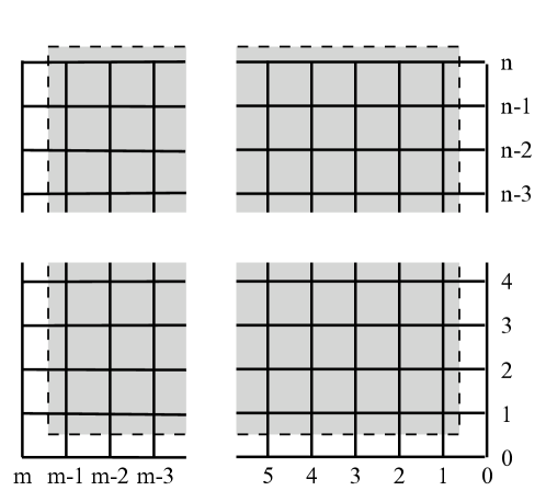
Figure 1: Nodes and their right-to-left, and bottom-to-top numbering.

3 Triangular strip matrices

In this paper we use matrices of a specific structure, which are called triangular strip matrices [51, 59], and which have been also mentioned in [1, 18]. We will need lower triangular strip matrices,

$$L_{N}=\left[\begin{array}[]{cccccc}\omega_{0}&0&0&0&\cdots&0\\ \omega_{1}&\omega_{0}&0&0&\cdots&0\\ \omega_{2}&\omega_{1}&\omega_{0}&0&\cdots&0\\ \ddots&\ddots&\ddots&\ddots&\cdots&\cdots\\ \omega_{N-1}&\ddots&\omega_{2}&\omega_{1}&\omega_{0}&0\\ \omega_{N}&\omega_{N-1}&\ddots&\omega_{2}&\omega_{1}&\omega_{0}\\ \end{array}\right],$$ (8)

and upper triangular strip matrices,

$$U_{N}=\left[\begin{array}[]{cccccc}\omega_{0}&\omega_{1}&\omega_{2}&\ddots&\omega_{N-1}&\omega_{N}\\ 0&\omega_{0}&\omega_{1}&\ddots&\ddots&\omega_{N-1}\\ 0&0&\omega_{0}&\ddots&\omega_{2}&\ddots\\ 0&0&0&\ddots&\omega_{1}&\omega_{2}\\ \cdots&\cdots&\cdots&\cdots&\omega_{0}&\omega_{1}\\ 0&0&0&\cdots&0&\omega_{0}\\ \end{array}\right],$$ (9)

A lower (upper) triangular strip matrix is completely described by its first column (row). Therefore, if we define the truncation operation, $\mbox{trunc}_{N}\left(\cdot\right)$, which truncates (in a general case) the power series $\varrho(z)$,

$$\varrho(z)=\sum_{k=0}^{\infty}\omega_{k}z^{k}$$ (10)

to the polynomial $\varrho_{N}(z)$,

$$\mbox{trunc}_{N}\left(\varrho(z)\right)\stackrel{{\scriptstyle\mbox{\scriptsize def}}}{{=}}\sum_{k=0}^{N}\omega_{k}z^{k}=\varrho_{N}(z),$$ (11)

then we can consider the function $\varrho(z)$ as a generating series for the set of lower (or upper) triangular matrices $L_{N}$ (or $U_{N}$), $N=1,2,\ldots$

It was shown in  [51] that operations with triangular strip matrices, such as addition, subtraction, multiplication, and inversion, can be expressed in the form of operations with their generating series (10).

Among properties of triangular strip matrices it should be noticed that if matrices $C$ and $D$ are both lower (upper) triangular strip matrices, then they commute:

$$CD=D\,C.$$ (12)

4 Kronecker matrix product

The Kronecker product $A\otimes B$ of the $n\times m$ matrix $A$ and the $p\times q$ matrix $B$

$$A=\left[\begin{array}[]{cccc}a_{11}&a_{12}&\ldots&a_{1m}\\ a_{21}&a_{22}&\ldots&a_{2m}\\ \vdots&\vdots&\ddots&\vdots\\ a_{n1}&a_{n2}&\ldots&a_{nm}\end{array}\right],\qquad B=\left[\begin{array}[]{cccc}b_{11}&b_{12}&\ldots&b_{1q}\\ b_{21}&b_{22}&\ldots&b_{2q}\\ \vdots&\vdots&\ddots&\vdots\\ b_{p1}&b_{p2}&\ldots&b_{pq}\end{array}\right],$$ (13)

is the $np\times mq$ matrix having the following block structure:

$$A\otimes B=\left[\begin{array}[]{cccc}a_{11}B&a_{12}B&\ldots&a_{1m}B\\ a_{21}B&a_{22}B&\ldots&a_{2m}B\\ \vdots&\vdots&\ddots&\vdots\\ a_{n1}B&a_{n2}B&\ldots&a_{nm}B\end{array}\right].$$ (14)

For example, if

$$A=\left[\begin{array}[]{cc}1&2\\ 0&-3\end{array}\right],\qquad B=\left[\begin{array}[]{ccc}1&2&3\\ 4&5&6\end{array}\right],$$ (15)

then

$$A\otimes B=\left[\begin{array}[]{rrrrrr}1&2&3&2&4&6\\ 4&5&6&8&10&12\\ 0&0&0&-3&-6&-9\\ 0&0&0&-12&-15&-18\end{array}\right].$$ (16)

Among many known interesting properties of the Kronecker product we would like to recall those that are important for the subsequent sections. Namely [63],

• if $A$ and $B$ are band matrices, then $A\otimes B$ is also a band matrix,

• if $A$ and $B$ are lower (upper) triangular, then $A\otimes B$ is also lower (upper) triangular.

We will also need two specific Kronecker products, namely the products $E_{n}\otimes A$ and $A\otimes E_{m}$, where $E_{n}$ is an $n\times n$ identity matrix. For example, if $A$ is a $2\times 3$ matrix

$$A=\left[\begin{array}[]{ccc}{\it a_{11}}&{\it a_{12}}&{\it a_{13}}\\ \vskip 6.0pt plus 2.0pt minus 2.0pt\cr{\it a_{21}}&{\it a_{22}}&{\it a_{23}}\end{array}\right]$$ (17)

then

$$E_{2}\otimes A=\left[\begin{array}[]{cccccc}{\it a_{11}}&{\it a_{12}}&{\it a_{13}}&0&0&0\\ \vskip 6.0pt plus 2.0pt minus 2.0pt\cr{\it a_{21}}&{\it a_{22}}&{\it a_{23}}&0&0&0\\ \vskip 6.0pt plus 2.0pt minus 2.0pt\cr 0&0&0&{\it a_{11}}&{\it a_{12}}&{\it a_{13}}\\ \vskip 6.0pt plus 2.0pt minus 2.0pt\cr 0&0&0&{\it a_{21}}&{\it a_{22}}&{\it a_{23}}\end{array}\right]$$ (18)

$$A\otimes E_{3}=\left[\begin{array}[]{ccccccccc}{\it a_{11}}&0&0&{\it a_{12}}&0&0&{\it a_{13}}&0&0\\ \vskip 6.0pt plus 2.0pt minus 2.0pt\cr 0&{\it a_{11}}&0&0&{\it a_{12}}&0&0&{\it a_{13}}&0\\ \vskip 6.0pt plus 2.0pt minus 2.0pt\cr 0&0&{\it a_{11}}&0&0&{\it a_{12}}&0&0&{\it a_{13}}\\ \vskip 6.0pt plus 2.0pt minus 2.0pt\cr{\it a_{21}}&0&0&{\it a_{22}}&0&0&{\it a_{23}}&0&0\\ \vskip 6.0pt plus 2.0pt minus 2.0pt\cr 0&{\it a_{21}}&0&0&{\it a_{22}}&0&0&{\it a_{23}}&0\\ \vskip 6.0pt plus 2.0pt minus 2.0pt\cr 0&0&{\it a_{21}}&0&0&{\it a_{22}}&0&0&{\it a_{23}}\end{array}\right]$$ (19)

This illustrates that left multiplication of $A_{n\times m}$ by $E_{n}$ creates an $n\times n$ block diagonal matrix by repeating the matrix $A$ on the diagonal, and that right multiplication of $A_{n\times m}$ by $E_{m}$ creates a sparse matrix made of $n\times m$ diagonal blocks.

5 Eliminators

The suggested method requires also the use of a certain type of matrices called eliminators [51], which are obtained from the $N\times N$ unit matrix $E$ by keeping only some of its rows and omitting all other rows: $S_{1}$ is obtained by omitting only the first row of $E$; $S_{2}$ is obtained by omitting only the second row; $S_{1,2}$ is obtained by omitting only the first and the second row of $E$; and, in general, $S_{r_{1},r_{2},\ldots,r_{k}}$ is obtained by omitting the rows with the numbers $r_{1},r_{2},\ldots,r_{k}$. In case of infinite matrices, similar matrices appeared in [10].

If $A$ is a square $N\times N$ matrix, then the product $S_{r_{1},r_{2},\ldots,r_{k}}A$ contains only rows of $A$ with the numbers different from $r_{1},r_{2},\ldots,r_{k}$. Similarly, the product $AS_{r_{1},r_{2},\ldots,r_{k}}^{T}$ contains only columns of $A$ with the numbers different from $r_{1},r_{2},\ldots,r_{k}$.

The following simple example illustrates the main property of eliminators:

$$A=\left[\begin{array}[]{lll}a_{11}&a_{12}&a_{13}\\ a_{21}&a_{22}&a_{23}\\ a_{31}&a_{32}&a_{33}\\ \end{array}\right];\qquad S_{1}=\left[\begin{array}[]{lll}0&1&0\\ 0&0&1\\ \end{array}\right];\qquad S_{1}\,A=\left[\begin{array}[]{lll}a_{21}&a_{22}&a_{23}\\ a_{31}&a_{32}&a_{33}\\ \end{array}\right];$$

$$A\,S_{1}^{T}=\left[\begin{array}[]{ll}a_{12}&a_{13}\\ a_{22}&a_{23}\\ a_{32}&a_{33}\\ \end{array}\right];\qquad S_{1}\,A\,S_{1}^{T}=\left[\begin{array}[]{ll}a_{22}&a_{23}\\ a_{32}&a_{33}\\ \end{array}\right].$$

6 Shifters

For some types of approximation of differential operators (for example, one of the approximations of the symmetric Riesz derivative below in this article) and especially for numerical solution of differential equations of arbitrary order (integer or fractional) with delays, it is convenient to introduce another special kind of matrices – shifters –, which will represent discrete shifts, like, for example, delays.

Shifters (although without using this term) were used in [51] for a simple generation of triangular strip matrices. There are shifters of two kinds: $(N+1)\times(N+1)$ matrices $E_{N,p}^{+}$, $p=1,\ldots N$, with ones on $p$-th diagonal above the main diagonal and zeroes elsewhere, and matrices $E_{N,p}^{-}$, $p=1,\ldots N$, with ones on $p$-th diagonal below the main diagonal and zeroes elsewhere. We also denote $E_{N,0}^{\pm}\equiv E_{N}$ the unit matrix.

The shift of all the coefficients in the triangular strip matrix $U_{N}$ in the south-west (bottom-left) direction can be easily written if we start with $U_{N+1}$ and then use shifters and eliminators:

$$_{-1}U_{N}=S_{1}\,E_{N+1,1}^{-}\,U_{N+1}\,E_{N+1,1}^{-}\,S_{N+1}^{T}$$ (20)

Similarly, the shift of all the coefficients in the triangular strip matrix $U_{N}$ in the north-east (top-right) direction can be easily obtained as:

$$_{+1}U_{N}=S_{N+1}\,E_{N+1,1}^{+}\,U_{N+1}\,E_{N+1,1}^{+}\,S_{1}^{T}$$ (21)

7 Discretization of ordinary fractional derivatives

It follows from [51], that the left-sided Riemann-Liouville or Caputo fractional derivative $v^{(\alpha)}(t)=\,_{0}D_{t}^{\alpha}v(t)$ can be approximated in all nodes of the equidistant discretization net $t=j\tau$ ($j=0,1,\ldots,n$) simultaneously with the help of the upper triangular strip matrix $B_{n}^{(\alpha)}$ as :

$$\Bigl{[}v_{n}^{(\alpha)}\;\;v_{n-1}^{(\alpha)}\;\;\ldots\;v_{1}^{(\alpha)}\;\;v_{0}^{(\alpha)}\Bigr{]}^{T}=B_{n}^{(\alpha)}\;\Bigl{[}v_{n}\;\;v_{n-1}\;\;\ldots\;v_{1}\;\;v_{0}\Bigr{]}^{T}$$ (22)

where

$$B_{n}^{(\alpha)}=\frac{1}{\tau^{\alpha}}\left[\!\!\begin{array}[]{cccccc}\omega^{(\alpha)}_{0}&\omega^{(\alpha)}_{1}&\ddots&\ddots&\omega^{(\alpha)}_{n-1}&\omega^{(\alpha)}_{n}\\ 0&\omega^{(\alpha)}_{0}&\omega^{(\alpha)}_{1}&\ddots&\ddots&\omega^{(\alpha)}_{n-1}\\ 0&0&\omega^{(\alpha)}_{0}&\omega^{(\alpha)}_{1}&\ddots&\ddots\\ \cdots&\cdots&\cdots&\ddots&\ddots&\ddots\\ 0&\cdots&0&0&\omega^{(\alpha)}_{0}&\omega^{(\alpha)}_{1}\\ 0&0&\cdots&0&0&\omega^{(\alpha)}_{0}\\ \end{array}\!\!\!\right]$$ (23)

$$\omega_{j}^{(\alpha)}=(-1)^{j}{\alpha\choose j},\qquad j=0,1,\ldots,n.$$ (24)

Similarly, the right-sided Riemann-Liouville or Caputo fractional derivative $v^{(\alpha)}(t)=\,_{t}D_{b}^{\alpha}v(t)$ can be approximated in all nodes of the equidistant discretization net $t=j\tau$ ($j=0,1,\ldots,n$) simultaneously with the help of the lower triangular strip matrix $F_{n}^{(\alpha)}$:

$$\Bigl{[}v_{n}^{(\alpha)}\;\;v_{n-1}^{(\alpha)}\;\;\ldots\;v_{1}^{(\alpha)}\;\;v_{0}^{(\alpha)}\Bigr{]}^{T}=F_{n}^{(\alpha)}\;\Bigl{[}v_{n}\;\;v_{n-1}\;\;\ldots\;v_{1}\;\;v_{0}\Bigr{]}^{T}$$ (25)

$$F_{n}^{(\alpha)}=\frac{1}{\tau^{\alpha}}\left[\!\!\begin{array}[]{cccccc}\omega^{(\alpha)}_{0}&0&0&0&\cdots&0\\ \omega^{(\alpha)}_{1}&\omega^{(\alpha)}_{0}&0&0&\cdots&0\\ \omega^{(\alpha)}_{2}&\omega^{(\alpha)}_{1}&\omega^{(\alpha)}_{0}&0&\cdots&0\\ \ddots&\ddots&\ddots&\ddots&\cdots&\cdots\\ \omega^{(\alpha)}_{n-1}&\ddots&\omega^{(\alpha)}_{2}&\omega^{(\alpha)}_{1}&\omega^{(\alpha)}_{0}&0\\ \omega^{(\alpha)}_{n}&\omega^{(\alpha)}_{n-1}&\ddots&\omega^{(\alpha)}_{2}&\omega^{(\alpha)}_{1}&\omega^{(\alpha)}_{0}\\ \end{array}\!\!\!\right]$$ (26)

The symmetric Riesz derivative of order $\beta$ can be approximated based on its definition (5) as a combination of the approximations (22) and (25) for the left- and right-sided Riemann-Liouville derivatives, or using the centred fractional differences approximation of the symmetric Riesz derivative suggested recently by Ortigueira [48, 49]. The general formula is the same:

$$\Bigl{[}v_{m}^{(\beta)}\;\;v_{m-1}^{(\beta)}\;\;\ldots\;v_{1}^{(\beta)}\;\;v_{0}^{(\beta)}\Bigr{]}^{T}=R_{m}^{(\beta)}\;\Bigl{[}v_{m}\;\;v_{m-1}\;\;\ldots\;v_{1}\;\;v_{0}\Bigr{]}^{T}$$ (27)

In the first case, the approximation for the left-sided Caputo derivative is taken one step ahead, and the approximation for the right-sided Caputo derivatve is taken one step back. This leads to the matrix

$$R_{m}^{(\beta)}=\frac{h^{-\alpha}}{2}\Bigl{[}\;_{-1}U_{m}+\,_{+1}U_{m}\Bigr{]}$$ (28)

In the second case (Ortigueira’s definition [48]) we have the following symmetric matix:

$$R_{m}^{(\beta)}=h^{-\beta}\left[\;\!\!\begin{array}[]{cccccc}\omega^{(\beta)}_{0}&\omega^{(\beta)}_{1}&\omega^{(\beta)}_{2}&\omega^{(\beta)}_{3}&\cdots&\omega^{(\beta)}_{m}\\ \omega^{(\beta)}_{1}&\omega^{(\beta)}_{0}&\omega^{(\beta)}_{1}&\omega^{(\beta)}_{2}&\cdots&\omega^{(\beta)}_{m-1}\\ \omega^{(\beta)}_{2}&\omega^{(\beta)}_{1}&\omega^{(\beta)}_{0}&\omega^{(\beta)}_{1}&\cdots&\omega^{(\beta)}_{m-2}\\ \ddots&\ddots&\ddots&\ddots&\cdots&\cdots\\ \omega^{(\beta)}_{m-1}&\ddots&\omega^{(\beta)}_{2}&\omega^{(\beta)}_{1}&\omega^{(\beta)}_{0}&\omega^{(\beta)}_{1}\\ \omega^{(\beta)}_{m}&\omega^{(\beta)}_{m-1}&\ddots&\omega^{(\beta)}_{2}&\omega^{(\beta)}_{1}&\omega^{(\beta)}_{0}\\ \end{array}\!\!\!\right]$$ (29)

$$\omega_{k}^{(\beta)}=\frac{(-1)^{k}\,\Gamma(\beta+1)\,\cos(\beta\pi/2)}{\Gamma(\beta/2-k+1)\,\Gamma(\beta/2+k+1)},\qquad k=0,1,\ldots,m$$ (30)

Both these approximations of symmetric Riesz derivatives give practically the same numerical results and in case of numerical solution of partial fractional differential equations lead to a well-posed matrix of the resulting algebraic system.

8 Discretization of partial derivatives in time and space

The simplest implicit discretization scheme for the classical diffusion equation is shown in Fig. 4, where the two nodes in time direction are used for approximating the time derivative, and the three points in spatial direction are used for the symmetric approximation of the the spatial derivative. The stencil in Fig. 4 involves therefore only two time layers. If we consider fractional-order time derivative, then we have to involve all time levels starting from the very beginning. This is shown in Fig. 4 for the case of five time layers.

Similarly, if in addition to fractional-order time derivative we also consider symmetric fractional-order spatial derivatives, then we have to use all nodes at the considered time layer from the leftmost to the rightmost spatial discretization node. This most general situation is shown in Fig. 4.

Let us consider the nodes $(ih,j\tau)$, $j=0,1,2,\ldots,n$, corresponding to all time layers at $i$-th spatial discretization node. It has been shown in [51] that all values of $\alpha$-th order time derivative of $u(x,t)$ at these nodes are approximated using the discrete analogue of differentiation of arbitrary order:

$$\Bigl{[}u_{i,n}^{(\alpha)}\;u_{i,n-1}^{(\alpha)}\;\ldots\;u_{i,2}^{(\alpha)}\;u_{i,1}^{(\alpha)}\;u_{i,0}^{(\alpha)}\Bigr{]}=B_{n}^{(\alpha)}\,\Bigl{[}u_{i,n}\;u_{i,n-1}\;\ldots\;u_{i,2}\;u_{i,1}\;u_{i,0}\Bigr{]}^{T}$$ (31)

In order to obtain a simultaneous approximation of $\alpha$-th order time derivative of $u(x,t)$ in all nodes shown in Fig. 1, we need to arrange all function values $u_{ij}$ at the discretization nodes to the form of a column vector:

$$u_{nm}=\Bigl{[}u_{m,n}\;u_{m-1,n}\;\ldots\;u_{1,n}\;u_{0,n}\;\hskip 80.00012pt$$

$$u_{m,n-1}\;u_{m-1,n-1}\;\ldots\;u_{1,n-1}\;u_{0,n-1}\;\hskip 25.00003pt$$

$$\ldots\ldots\ldots\hskip 110.00017pt$$

$$u_{m,1}\;u_{m-1,1}\;\ldots\;u_{1,1}\;u_{0,1}\;\hskip 30.00005pt$$

$$u_{m,0}\;u_{m-1,0}\;\ldots\;u_{1,0}\;u_{0,0}\;\Bigr{]}^{T}$$ (32)

In visual terms of Fig. 1, we first take the nodes of $n$-th time layer, then the nodes of $(n-1)$-th time layer, and so forth, and put them in this order in a vertical column stack.

The matrix that transforms the vector $U_{nm}$ to the vector $U_{t}^{(\alpha)}$ of the partial fractional derivative of order $\alpha$ with respect to time variable can be obtained as a Kronecker product of the matrix $B_{n}^{(\alpha)}$, which corresponds to the fractional ordinary derivative of order $\alpha$ (recall that $n$ is the number of time steps), and the unit matrix $E_{m}$ (recall that $m$ is the number of spatial discretization nodes):

$$T_{mn}^{(\alpha)}=B_{n}^{(\alpha)}\otimes E_{m}$$ (33)

This is illustrated in Fig. 6, where the nodes denoted as white and gray are used to approximate the fractional-oder time derivative at the node shown in gray.

Similarly, the matrix that transforms the vector $U$ to the vector $U_{x}^{(\beta)}$ of the partial fractional derivative of order $\beta$ with respect to spatial variable can be obtained as a Kronecker product of the unit matrix $E_{n}$ (recall that $n$ is the number of spatial discretization nodes), and the matrix $R_{m}^{(\beta)}$, which corresponds to a symmetric Riesz ordinary derivative of order $\beta$ [48, 49] (recall that $m$ is the number of time steps):

$$S_{mn}^{(\alpha)}=E_{n}\otimes R_{n}^{(\beta)}$$ (34)

This is also illustrated in Fig. 6, where the nodes denoted as black and gray (corresponding to all discretization nodes from the leftmost to the rightmost one) are used to approximate the symmetric fractional-order Riesz derivative at the same node shown in gray.

Having these approximations for partial fractional derivatives with respect to both variables, we can immediately discretize the general form of the fractional diffusion equation by simply replacing the derivatives with their discrete analogs (Fig. 6). Namely, the equation

$${}_{0}^{C}D_{t}^{\alpha}u-\chi\frac{\partial^{\beta}u}{\partial|x|^{\beta}}=f(x,t)$$ (35)

is discretized as

$$\Bigl{\{}B_{n}^{(\alpha)}\otimes E_{m}-\chi\,E_{n}\otimes R_{m}^{(\beta)}\Bigr{\}}u_{nm}=f_{nm},$$ (36)

and the matrix of this system has the structure shown in Fig. 7.

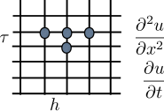
Figure 2: A stencil for integer-order derivatives.

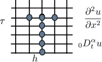
Figure 3: A stencil in case of fractional time derivative.

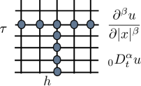
Figure 4: A stencil in case of fractional time and spatial derivatives.

9 Initial and boundary conditions

Initial and boundary conditions must be equal to zero. If it is not so, then an auxiliary unknown function must be introduced, which satisfies the zero initial and boundary conditions. In this way, the non-zero initial and boundary conditions moves to the right-hand side of the equation for the new unknown function.

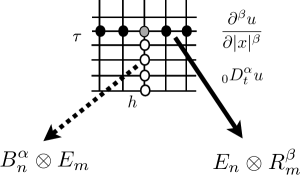
Figure 5: Discretization of partial derivatives.

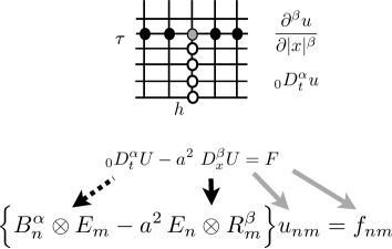
Figure 6: Discretization of partial derivatives and of the equation

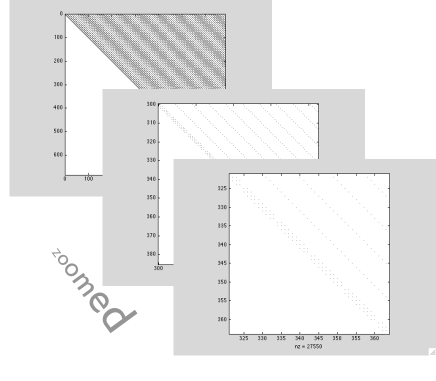
Figure 7: The structure of the matrix of the resulting algebraic system.

10 Implementation in MATLAB

We provide a set of MATLAB routines for implementing the suggested method [53]. The function BCRECUR returns the values of the coefficients that appear in the fractional difference approximations of fractional derivatives. The function BAN returns the matrix for the backward difference approximation of the left-sided ordinary fractional derivative, the function FAN returns the matrix for approximating the right-sided ordinary fractional derivative, and the functions RANSYM and RANORT return the matrices for approximating the symmetric Riesz using the formulas (28) and (29), respectively. The function ELIMINATOR returns the eliminator matrix, and the function SHIFT implements the operations (20) and (21).

The use of these routines is illustrated by the demo functions FRACDIFFDEMOU, which implements Examples 1 and 2 below, FRACDIFFDEMOY, which implements Examples 3 and 4, and FRACDIFFDEMOYDELAY, which implements Example 5.

11 Examples

In this section we introduce several examples illustrating the use of the suggested method.

First, we demonstrate that for the classical integer-order diffusion equation our method gives proper results, which are in agreement with the analytical and numerical solutions provided in [46].

Second, we obtain the numerical solution of a time-fractional diffusion equation. This solution is in perfect agreement with the numerical solution obtained in the very recent work [55] by a different approach.

Then we consider fractional diffusion equation with spatial fractional derivative. The fractional derivative with respect to the spatial variable is considered as a Riesz fractional derivative.

After that, we show the results of numerical solution of a general fractional diffusion equation, where time and spatial derivatives are both of fractional order – the time fractional derivative is a left-sided Riemann–Liouville derivative, and the spatial fractional derivative is a Riesz fractional derivatie.

Finally, we demonstrate that consideration of partial differential equations with fractional derivatives and delays is equally simple in the framework of the suggested general approach.

In all examples, the spatial interval is finite.

11.1 Example 1: Classical diffusion equation

Let us start with the classical problem [46]:

$$\frac{\partial u}{\partial t}=\frac{\partial^{2}u}{\partial x^{2}}$$ (37)

$$u(0,t)=0,\quad u(1,t)=0$$ (38)

$$u(x,0)=4x(1-x)$$ (39)

To reduce this problem to a problem with zero initial conditions (the boundary conditions are already zero), let us introduce an auxiliary function

$$y(x,t)=u(x,t)-u(x,0)$$ (40)

It follows from (40) and (37)–(39) that the function $y(x,t)$ must satisfy

$$\frac{\partial y}{\partial t}-\frac{\partial^{2}y}{\partial x^{2}}=f(x,t),\qquad(\mbox{with }f(x,t)\equiv 8)$$ (41)

$$y(0,t)=0,\quad y(1,t)=0;\qquad\quad y(x,0)=0.$$ (42)

The problem (41)–(42) can be discretized using the described method (see Fig. 6), which gives

$$\Bigl{\{}B_{n}^{(1)}\otimes E_{m}-\,E_{n}\otimes R_{m}^{(2)}\Bigr{\}}y_{nm}=f_{nm}$$ (43)

where $m$ is the number of spatial discretization intervals and $n$ is the number of time steps.

To obtain the system for finding the unknown values of $y_{nm}$ for the inner nodes of the discretization net, we have to use the initial and boundary conditions. Since they all are zero, it is sufficient to delete the corresponding rows and columns in the system (43), which is easily done with the help of eliminators.

The result of computation of $y(x,t)$ for the spatial step $h=0.1$ and the time step $\tau=h^{2}/6$ is shown in Fig. 8 (on the left) for $n=37$ time steps. These values were chosen for the purpose of comparison with the results from [46]. Using (40), we can compute $u(x,t)$, and the result is shown in Fig. 8 (on the right). The values of $u(x,t)$ are in perfect agreement with the values given in [46] for the same values of $h$, $\tau$, and $n$.

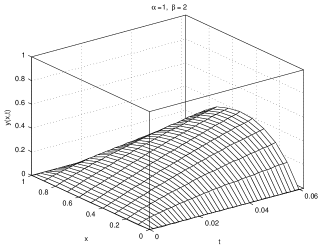
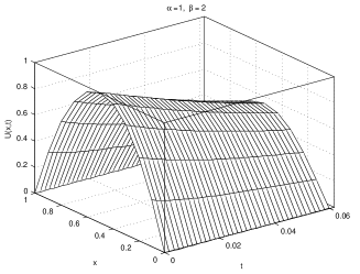
Figure 8: Solutions $y(x,t)$ (left) and $u(x,t)$ (right) of Example 1, with the same values of parameters as in [46].

11.2 Example 2: Diffusion equation with time fractional derivative

Now let us consider the equation with the Caputo fractional-order time derivative:

$$_{0}^{C}\!D_{t}^{\alpha}u=\frac{\partial^{2}u}{\partial x^{2}}$$ (44)

$$u(0,t)=0,\quad u(1,t)=0$$ (45)

$$u(x,0)=4x(1-x)$$ (46)

Since the Caputo derivative of a constant is zero [2, 50], for the auxiliary function $y(x,t)$ defined by equation (40) we obtain a problem with zero initial and boundary conditions similar to (41)–(42):

$${}_{0}^{C}\!D_{t}^{\alpha}y-\frac{\partial^{2}y}{\partial x^{2}}=f(x,t),\qquad(\mbox{with }f(x,t)\equiv 8)$$ (47)

$$y(0,t)=0,\quad y(1,t)=0;\qquad\quad y(x,0)=0$$ (48)

This problem can be discretized in the same manner as the previous one (refer to Fig. 6), with the only difference that instead of the first-order time derivative we have now a derivative of order $\alpha$:

$$\Bigl{\{}B_{n}^{(\alpha)}\otimes E_{m}-\,E_{n}\otimes R_{m}^{(2)}\Bigr{\}}y_{nm}=f_{nm}$$ (49)

where $m$ is the number of spatial discretization intervals and $n$ is the number of time steps.

As above, the use of the zero initial conditions means that the corresponding rows and columns in the system (49) are removed with the help of eliminators.

The results of computations of $y(x,t)$ and then $u(x,t)$ for $\alpha=1$, $\alpha=0.7$, $\alpha=0.5$ with $h=0.05$ and $\tau=h^{2}/6$ are shown in Fig.  9. The structure of the matrix is the same as shown in Fig. 7.

Obviously, for $\alpha=1$ we have the classical case and the same plots as in Fig. 8, and therefore Example 1 is a particular case of Example 2. As $\alpha$ goes to zero, the function $y(x,t)$ slowly tends to $u(x,0)=4x(1-x)$ for all $t$. This is also not a surprize, because, indeed, for $\alpha=0$ the function $y(x,t)$ does not depend on $t$ and therefore must satisfy

$$y^{\prime\prime}(x)+8=0,\quad y(0)=y(1)=0,$$

which has the solution $y(x)=4x(1-x)$.

It should be noted that almost the same problem as (44)–(46) was numerically solved in [55] using a very different approach. The initial condition in [55] was $u(x,0)=x(1-x)$. Scaling the plots in figures 1 and 2 in [55] by the factor of 4, we obtain the plots which are practically identical with our results for $u(x,t)$ shown in Fig. 9. For this comparison we considered the shorter interval $0\leq t\leq 0.02$ used in [55].

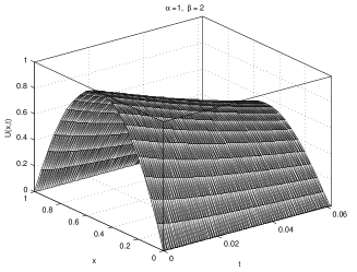
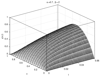
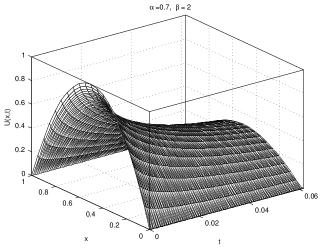
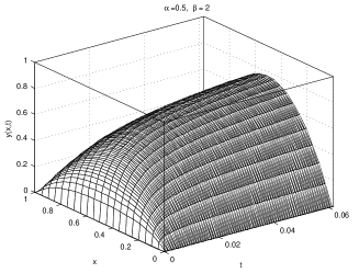
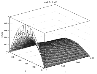
Figure 9: Solutions $y(x,t)$ (left column) and $u(x,t)$ (right column) of Example 2, for $\alpha=1$ (top), $\alpha=0.7$ (middle) and $\alpha=0.5$ (bottom), with spatial step $h=0.05$ and time step $\tau=h^{2}/6$.

11.3 Example 3: Diffusion equation with spatial fractional derivative

Let us now focus on the role of spatial fractional derivative. For clarity, let us directly write the following analog of the problem (41)–(42) for determining the function $y(x,t)$:

$$\frac{\partial y}{\partial t}-\frac{\partial^{\beta}y}{\partial|x|^{\beta}}=f(x,t),\qquad(\mbox{with }f(x,t)\equiv 8)$$ (50)

$$y(0,t)=0,\quad y(1,t)=0;\qquad\quad y(x,0)=0.$$ (51)

where $1<\beta\leq 2$. The right-hand side is the same as in (41), but instead of second order spatial derivative we deal with the Riesz-Caputo fractional derivative.

The problem (50)–(51) can be discretized using the described method (see Fig. 6), which gives

$$\Bigl{\{}B_{n}^{(1)}\otimes E_{m}-\,E_{n}\otimes R_{m}^{(\beta)}\Bigr{\}}y_{nm}=f_{nm}$$ (52)

where $m$ is the number of spatial discretization intervals and $n$ is the number of time steps, and the corresponding rows and columns in the system (52) are removed with the help of eliminators.

The results of computations for four different values of $\beta$ are shown in Fig. 10.

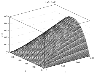
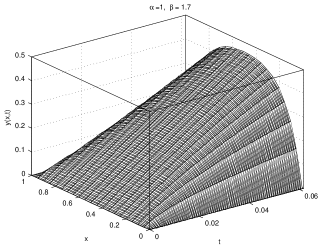
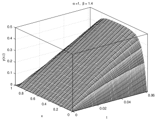
Figure 10: Solutions $y(x,t)$ (left column) of Example 3, for $\beta=2$ (top-left), $\beta=1.7$ (top-right), $\beta=1.4$ (bottom-left), and $\beta=1.1$ (bottom-right), with spatial step $h=0.05$ and time step $\tau=h^{2}/6$.

11.4 Example 4: General fractional diffusion equation

Now we can illustrate that the method works also in the case when both derivatives are of fractional order. Let us consider the most general situation:

$$_{0}^{C}\!D_{t}^{\alpha}y-\frac{\partial^{\beta}y}{\partial|x|^{\beta}}=f(x,t),\qquad(\mbox{with }f(x,t)\equiv 8)$$ (53)

$$y(0,t)=0,\quad y(1,t)=0;\qquad\quad y(x,0)=0.$$ (54)

The right-hand side is the same as in (41) and (50), but now both derivatives are allowed to be of non-integer order.

The problem (53)–(54) can be discretized using the described method (see Fig. 6), which gives

$$\Bigl{\{}B_{n}^{(\alpha)}\otimes E_{m}-\,E_{n}\otimes R_{m}^{(\beta)}\Bigr{\}}y_{nm}=f_{nm}$$ (55)

where $m$ is the number of spatial discretization intervals and $n$ is the number of time steps, and the corresponding rows and columns in the system (55) are as in all previous examples removed with the help of eliminators.

The results of computations for some sample combinations of non-integer orders $\alpha$ and different values of $\beta$ are shown in Fig. 11.

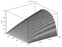
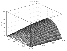
Figure 11: Solutions $y(x,t)$ of Example 4, for $\alpha=0.7$ and $\beta=1.4$ (left), $\alpha=0.7$ and $\beta=1.8$ (middle), $\alpha=0.7$ $\beta=2$ (right), with spatial step $h=0.05$ and time step $\tau=h^{2}/6$.

11.5 Example 5: Fractional diffusion equation with delay

Finally, let us consider the equation with two Caputo fractional-order time derivatives, of which one is with delay $\delta$ (we do not go into the physical interpretation of this equation, because physical interpretation of a delayed fractional derivative is not known so far, but use it for demonstrating how broad can be the field of application of our approach):

$$\frac{1}{2}\left\{\;{}_{0}^{C}\!D_{t}^{\alpha}y+\;_{0}^{C}\!D_{t-\delta}^{\gamma}y\right\}-\frac{\partial^{\beta}y}{\partial|x|^{\beta}}=f(x,t)\qquad(\mbox{with }f(x,t)\equiv 8)$$ (56)

$$y(0,t)=0,\quad y(1,t)=0\quad y(x,0)=0$$ (57)

Obviously, for $\gamma=\alpha$ and $\delta=0$ we have the equation considered in Example 2. Let us select the discretization step so that $\delta$ is a multiple of the time step $\tau$: $\delta=k\tau$. Then the problem (56)–(57) can be discretized using the described method (see Fig. 6 and the equation (21)), which gives:

$$\Bigl{\{}\frac{1}{2}\left(B_{n}^{(\alpha)}\otimes E_{m}+\,\,_{+k}B_{n}^{(\gamma)}\otimes E_{m}\right)-\,\,E_{n}\otimes R_{m}^{(\beta)}\Bigr{\}}y_{nm}=f_{nm}$$ (58)

$${}_{+k}B_{n}^{(\gamma)}=S_{n+1,\dots,n+k}\,E_{n+k,k}^{+}\,B_{n+k}^{(\gamma)}\,E_{n+k,k}^{+}\,S_{1,\ldots,k}^{T}$$

where, as above, $m$ is the number of spatial discretization intervals and $n$ is the number of time steps, $k$ is the number of time steps corresponding to the delay $\delta$, and the appropriate rows and columns in the system (58) are as in all previous examples are to removed with the help of eliminators.

The results of computations for a sample combination of non-integer orders $\alpha$, $\beta$ and $\gamma$ and some delays $\delta$ represented by the parameter $k$ are shown in Fig. 12.

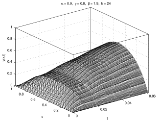
Figure 12: Solutions $y(x,t)$ (left column) of Example 5, for $\alpha=0.9$, $\gamma$ = 0.8, $\beta=1.9$, for delays $\delta_{k}=k\tau$, k = 6, 12, 24, 36.

12 Conclusion

The suggested method represents a unifying approach to numerical solution of partial differential equations of both integer and non-integer order, including equations with delays.

For the sake of clarity, in this article we considered the case of one spatial variable. However, the suggested method can be easily extended to the case of two and three spatial variables by repeatedly applying the triangular strip matrix representations of fractional-order operators in combination with the Kronecker matrix product.

The problems considered in this article are linear, so the resulting systems of algebraic equations are linear as well. However, the suggested approach can be extended to the case of nonlinear problems, too.

The suggested method can be used also for solving partial fractional differential equations appearing from the Laplace equation by replacing second order spatial derivatives with fractional Riesz derivatives.

The suggested method can be used also for partial fractional FDEs of variable and distributed order(s) and for equations with delays.

Appendix: sample evaluation of the symmetric Riesz fractional derivative

For $\phi(x)=x(1-x)$ and the order of differentiation $1<\beta<2$ the left-sided Riemann-Liouville fractional derivative (6) of the function $\phi(x)$ is

$${}_{0}D_{x}^{\beta}\phi(x)=\frac{x^{1-\beta}}{\Gamma(2-\beta)}-\frac{2\,x^{2-\beta}}{\Gamma(3-\beta)}.$$ (59)

Similarly, the right-sided Riemann-Liouville derivative (7) of $\phi(x)$ is

$${}_{x}D_{1}^{\beta}\phi(x)=\frac{(1-x)^{1-\beta}}{\Gamma(2-\beta)}-\frac{2\,(1-x)^{2-\beta}}{\Gamma(3-\beta)}.$$ (60)

Therefore, the symmetric Riesz fractional derivative (5) of the function $\phi(x)$ is:

$$\frac{d^{\beta}\phi}{d|x|^{\beta}} = \frac{1}{2}\left\{\,{}_{0}D_{x}^{\beta}\phi(x)+\,_{x}D_{1}^{\beta}\phi(x)\right\}$$ (61)

$$= \frac{x^{1-\beta}+(1-x)^{\beta}}{2\,\Gamma(2-\beta)}-\frac{x^{2-\beta}+(1-x)^{2-\beta}}{\Gamma(3-\beta)}.$$ (62)

References

- [1] B. V. Bulgakov, Kolebaniya (Vibrations), Gostekhizdat, Moscow, 1954.
- [2] M. Caputo, Elasticità e dissipazione, Zanichelli, Bologna, 1969.
- [3] A. Chechkin, V. Gonchar, R. Gorenflo, N. Korabel, I. Sokolov, Generalized fractional diffusion equations for accelerating subdiffusion and truncated levy flights, Physical Review E 78 (2008) Article 021111.
- [4] A. Chechkin, V. Gonchar, J. Klafter, R. Metzler, L. Tanatarov, Stationary states of non-linear oscillators driven by Lévy noise, Chemical Physics 284 (1–2) (2002) 233—251.
- [5] A. Chechkin, V. Gonchar, M. Szydłowsky, Fractional kinetics for relaxation and superdiffusion in magnetic field, Physics of Plasmas 9 (1) (2002) 78–88.
- [6] A. Chechkin, V. Y. Gonchar, J. Klafter, R. Metzler, Fundamentals of Lévy flight processes., Advances in Chemical Physics 133 (2006) 439–496.
- [7] A. Chechkin, R. Gorenflo, I. Sokolov, Retarding subdiffusion and accelerating superdiffusion governed by distributed order fractional diffusion equations, Physical Review E 66 (4, art 046129) (2002) 1—7.
- [8] A. Chechkin, R. Gorenflo, I. Sokolov, Fractional diffusion in inhomogeneous media, Journal of Physics A: Mathematical and General 38 (42) (2005) L679—L684.
- [9] A. Chechkin, R. Gorenflo, I. Sokolov, V. Gonchar, Distributed order time fractional diffusion equation, Fractional Calculus and Applied Analysis 6 (3) (2003) 259—279.
- [10] R. G. Cooke, Infinite Matrices and Sequence Spaces, Fizmatgiz, Moscow, 1960.
- [11] D. del Castillo-Negrete, Fractional diffusion models of nonlocal transport, Physics of Plasmas 13 (8) (2006) Article 082308.
- [12] D. del Castillo-Negrete, B. A. Carreras, V. E. Lynch, Front dynamics in reaction-diffusion systems with Lévy flights: A fractional diffusion approach, Phys. Rev. Lett. 91 (1) (2003) Article 018302.
- [13] D. del Castillo-Negrete, B. A. Carreras, V. E. Lynch, Nondiffusive transport in plasma turbulence: A fractional diffusion approach, Phys. Rev. Lett. 94 (2005) Article 065003.
- [14] D. del Castillo-Negrete, V. Gonchar, A. Chechkin, Fluctuation-driven directed transport in presence of Lévy flights, Physica A 27 (2008) 6693–6704.
- [15] V. J. Ervin, J. P. Roop, Variational formulation for the stationary fractional advection dispersion equation, Numerical Methods for Partial Differential Equations 22 (3) (2005) 558–576.
- [16] V. J. Ervin, J. P. Roop, Variational solution of fractional advection dispersion equations on bounded domains in , Numerical Methods for Partial Differential Equations 23 (2) (2006) 256–281.
- [17] R. Friedrich, Statistics of Lagrangian velocities in turbulent flows, Physical Review Letters 90 (8) (2003) Article 084501.
- [18] F. R. Gantmakher, Theory of Matrices, Nauka, Moscow, 1988.
- [19] R. Gorenflo, E. Abdel-Rehim, Discrete models of time-fractional diffusion in a potential well, Fractional Calculus and Applied Analysis 8 (2) (2005) 173–200.
- [20] R. Gorenflo, G. De Fabritiis, F. Mainardi, Discrete random walk models for symmetric Lévy–Feller diffusion processes, Physica A 269 (1999) 79–89.
- [21] R. Gorenflo, F. Mainardi, Random walk models for space-fractional diffusion processes, Fractional Calculus and Applied Analysis 1 (2) (1998) 167–192.
- [22] R. Gorenflo, F. Mainardi, Random walk models approximating symmetric space fractional diffusion processes, Problems in Mathematical Physics 121 (2001) 120–145.
- [23] R. Gorenflo, F. Mainardi, D. Moretti, G. Pagnini, P. Paradisi, Discrete random walk models for space-time fractional diffusion, Chemical Physics 284 (1–2) (2002) 521–541.
- [24] R. Gorenflo, F. Mainardi, D. Moretti, G. Pagnini, P. Paradisi, Fractional diffusion: probability distributions and random walk models., Physica A 305 (1–2) (2002) 106–112.
- [25] R. Gorenflo, F. Mainardi, D. Moretti, P. Paradisi, Time fractional diffusion: A discrete random walk approach., Nonlinear Dynamics 29 (2002) 129–143.
- [26] E. Heinsalu, M. Patriarca, I. Goychuk, H. P., Use and abuse of a fractional Fokker-Planck dynamics for time-dependent driving, Physical Review Letters 99 (2007) Article 120602.
- [27] N. Heymans, I. Podlubny, Physical interpretation of initial conditions for fractional differential equations with Riemann-Liouville fractional derivatives, Rheologica Acta 45 (5) (2006) 765–771.
- [28] R. Klages, G. Radons, I. M. Sokolov (eds.), Anomalous Transport, Wiley-VCH, Berlin, 2008.
- [29] T. Langlands, B. Henry, The accuracy and stability of an implicit solution method for the fractional diffusion equation, Journal of Computational Physics 205 (2) (2005) 719–736.
- [30] J. Liang, Y.-Q. Chen, Hybrid symbolic and numerical simulation studies of time-fractional order wave-diffusion systems, International Journal of Control 79 (11) (2006) 1462–1470.
- [31] Y. Lin, C. Xu, Finite difference/spectral approximations for the time-fractional diffusion equation, Journal of Computational Physics 225 (2) (2007) 1533–1552.
- [32] F. Liu, V. Anh, I. Turner, Numerical solution of the space fractional Fokker–Planck equation, Journal of Computational and Applied Mathematics 166 (1) (2004) 209–219.
- [33] Q. Liu, F. Liu, I. Turner, V. Anh, Approximation of the Levy–Feller advection-dispersion process by random walk and finite difference method, Journal of Computational Physics 222 (1) (2007) 57–70.
- [34] J.-F. Lu, A. Hanyga, Wave field simulation for heterogeneous porous media with singular memory drag force, Journal of Computational Physics 208 (2) (2005) 651–674.
- [35] V. E. Lynch, B. A. Carreras, D. del Castillo-Negrete, K. Ferreira-Mejias, Numerical methods for the solution of partial differential equations of fractional order, Journal of Computational Physics 192 (2003) 406–421.
- [36] F. Mainardi, Y. Luchko, G. Pagnini, The fundamental solution of the space-time fractional diffusion equation, Fractional Calculus and Applied Analysis 4 (2) (2001) 153–192.
- [37] F. Mainardi, A. Mura, G. Pagnini, R. Gorenflo, Time-fractional diffusion of distributed order, Journal of Vibration and Control 14 (9–10) (2008) 1267–1290.
- [38] M. Meerschaert, D. Benson, B. Bäumer, Multidimensional advection and fractional dispersion, Physical Review E 59 (5) (1999) 5026–5028.
- [39] M. Meerschaert, H.-P. Scheffler, C. Tadjeran, Finite difference methods for two-dimensional fractional dispersion equation, Journal of Computational Physics 211 (2006) 249–261.
- [40] M. Meerschaert, C. Tadjeran, Finite difference approximations for fractional advection-dispersion equations, Journal of Computational and Applied Mathematics 172 (1) (2004) 65–77.
- [41] M. Meerschaert, C. Tadjeran, Finite difference approximations for two-sided space-fractional partial differential equations, Applied Numerical Mathematics 56 (2006) 80–90.
- [42] M. M. Meerschaert, H.-P. Scheffler, C. Tadjeran, Finite difference methods for two-dimensional fractional dispersion equation, Journal of Computational Physics 211 (1) (2006) 249–261.
- [43] R. Metzler, E. Barkai, J. Klafter, Deriving fractional Fokker–Planck equations from a generalized master equation, Europhysics Letters 46 (4) (1999) 431–436.
- [44] R. Metzler, J. Klafter, The random walk’s guide to anomalous diffusion: a fractional dynamics approach, Phys. Reports. 339 (1) (2000) 1–77.
- [45] R. Metzler, J. Klafter, The restaurant at the end of the random walk: recent developments in the description of anomalous transport by fractional dynamics, Journ. Phys. A: Math. Gen. 37 (2) (2004) R161–R208.
- [46] W. E. Milne, Numerical Solution of Differential Equations, Wiley, New York, 1953.
- [47] K. B. Oldham, J. Spanier, The Fractional Calculus, Academic Press, New York, 1974.
- [48] M. D. Ortigueira, Riesz potential operators and inverses via fractional centred derivatives, International Journal of Mathematics and Mathematical Sciences Article ID 48391 (2006) 1–12.
- [49] M. D. Ortigueira, A. G. Batista, On the relation between the fractional Brownian motion and the fractional derivatives, Physics Letters A 372 (2008) 958–968.
- [50] I. Podlubny, Fractional Differential Equations, Academic Press, San Diego, 1999.
- [51] I. Podlubny, Matrix approach to discrete fractional calculus, Fractional Calculus and Applied Analysis 3 (4) (2000) 359–386.
- [52] I. Podlubny, Geometric and physical interpretation of fractional integration and fractional differentiation, Fractional Calculus and Applied Analysis 5 (4) (2002) 367–386.
- [53] I. Podlubny, A. Chechkin, T. Skovranek, Y. Chen, B. Vinagre Jara, Matrix approach to discretization of ODEs and PDEs of arbitrary real order, http://www.mathworks.com/matlabcentral/fileexchange/22071 (November 12, 2008).
- [54] A. Saichev, G. Zaslavsky, Fractional kinetic equations: solutions and applications, Chaos 7 No4 (1997) 753–764.
- [55] R. Scherer, S. L. Kalla, L. Boyadjiev, B. Al-Saqabi, Numerical treatment of fractional heat equations, Applied Numerical Mathematics 58 (8) (2008) 1212–1223.
- [56] I. Sokolov, J. Klafter, A. Blumen, Fractional kinetics, Physics Today 55 (2002) 48–54.
- [57] I. M. Sokolov, J. Klafter, Field-induced dispersion in subdiffusion, Physical Review Letters 97 (2006) Article 140602.
- [58] D. Stanescu, D. Kim, W. A. Woyczynski, Numerical study of interacting particles approximation for integro-differential equations, Journal of Computational Physics 206 (2) (2005) 706–726.
- [59] D. A. Suprunenko, R. I. Tyshkevich, Commutative Matrices, Nauka i Tekhnika, Minsk, 1966.
- [60] C. Tadjeran, M. M. Meerschaert, A second-order accurate numerical method for the two-dimensional fractional diffusion equation, Journal of Computational Physics 220 (2) (2007) 813–823.
- [61] C. Tadjeran, M. M. Meerschaert, H.-P. Scheffler, A second-order accurate numerical approximation for the fractional diffusion equation, Journal of Computational Physics 213 (1) (2006) 205–213.
- [62] P. P. Valko, J. Abate, Numerical inversion of 2-d Laplace transforms applied to fractional diffusion equation, Applied Numerical Mathematics 53 (2005) 73–88.
- [63] C. F. van Loan, The ubiquitous Kronecker product, Journal of Computational and Applied Mathematics 123 (2000) 85–100.
- [64] A. Weron, M. Magdziarz, K. Weron, Modeling of subdiffusion in space-time-dependent force fields beyond the fractional Fokker-Planck equation, Physical Review E 77 (2008) Article 036704.
- [65] Z. Yong, D. A. Benson, M. M. Meerschaert, H.-P. Scheffler, On using random walks to solve the space-fractional advection-dispersion equations, Journal of Statistical Physics 123 No.1 (2006) 89–110.
- [66] L. Yuan, O. P. Agrawal, A numerical scheme for dynamic systems containing fractional derivatives, Journal of Vibration and Acoustics 124 (2) (2002) 321–324.
- [67] S. Yuste, Weighted average finite difference methods for fractional diffusion equations, Journal of Computational Physics 216 (1) (2006) 264–274.
- [68] G. Zaslavsky, Chaos, fractional kinetics, and anomalous transport, Phys. Rep. 371 (1) (2002) 461–580.