Improved equations for eccentricity generation in hierarchical triple systems

Abstract

In a series of papers, we developed a technique for estimating the inner eccentricity in hierarchical triple systems, with the inner orbit being initially circular. However, for certain combinations of the masses and the orbital elements, the secular part of the solution failed. In the present paper, we derive a new solution for the secular part of the inner eccentricity, which corrects the previous weakness. The derivation applies to hierarchical triple systems with coplanar and initially circular orbits. The new formula is tested numerically by integrating the full equations of motion for systems with mass ratios from ${10^{-3}\hskip 5.69046pt\mbox{to}\hskip 5.69046pt10^{3}}$. We also present more numerical results for short term eccentricity evolution, in order to get a better picture of the behaviour of the inner eccentricity.

Key words: Celestial mechanics, binaries:general, binaries:close.

1 INTRODUCTION

Generally, stars have a tendency to form groups of different multiplicity, from the smallest possible (binary systems) up to large groups, like globular clusters with a population of the order of ${10^{7}}$ stars. Observations give values for the frequency of multiple stars in the galactic field of up to $70\%,$ (Kiseleva-Eggleton ${\&}$ Eggleton 2001 and references therein). Most of the multiple systems seem to be hierarchical (e.g. Tokovinin 1997, Kiseleva-Eggleton ${\&}$ Eggleton 2001).

A hierarchical triple system consists of a binary system and a third body on a wider orbit. The motion of such a system can be pictured as the motion of two binaries: the binary itself (inner binary) and the binary which consists of the third body and the centre of mass of the inner binary (outer binary). For most hierarchical triple stars, the period ratio ${X}$ is of the order of 100 and these systems are probably very stable dynamically. However, there are systems with much smaller period ratios, like the system HD 109648 with ${X=22}$ (Jha et al. 2000), the ${\lambda}$ Tau system, with $X=8.3$ (Fekel ${\&}$ Tomkin 1982) and the CH Cyg system with $X=7.0$ (Hinkle et al. 1993).

When the inner pair of a hierarchical triple stellar system is a close binary system, i.e. the separation between the components is comparable to the radii of the bodies, the evolution of the inner binary can depend very sensitively on the separation of its components and this in turn is affected by the third body. Thus, a slight change in the separation of the binary stars can cause drastic changes in processes such as tidal friction and dissipation, mass transfer, accretion and mass loss due to a stellar wind, which may result in changes in stellar structure and evolution. For instance, an eccentricity of only ${\sim 0.001}$ can be important in a semidetached binary (Kisela, Eggleton ${\&}$ Mikkola 1998). A comprehensive summary of those topics can be found in Eggleton (2006).

In a close binary, the orbit is expected to become circular eventually, due to tidal friction. However this is not possible when the binary motion is affected by the perturbations of a third companion (Mazeh ${\&}$ Shaham 1979, Mazeh 2008). Eggleton and Kiseleva (1996), based on results from numerical integrations of coplanar, prograde and initially circular orbits of hierarchical triple systems, derived the following empirical formula for the mean inner eccentricity:

$$\bar{e}_{{\rm in}}=\frac{A}{X^{1.5}\sqrt{X-B}},$$ (1)

where ${A}$ and ${B}$ depend on the mass ratios.

Equation (1) was confirmed analytically by Georgakarakos (2002). Moreover, the analytic derivation was generalized to hierarchical triple stellar systems with other orbital characteristics (Georgakarakos 2003 and 2004). Subsequently, some of the formulae were also tested for systems with planetary mass ratios (Georgakarakos 2006).

In the present paper, we deal with a problem that had to do with the secular part of our analytical solution and we manage to obtain a new formula which is free of that problem and gives improved results for certain cases. The new derivation applies to systems with initially circular and coplanar orbits, i.e. the type of systems we dealt with in Georgakarakos (2002). The new formula is tested numerically for systems with stellar and planetary mass ratios.

Other recent work on the dynamics of hierarchical triple systems includes the work done by Krymolowski ${\&}$ Mazeh (1999), Ford, Kozinsky ${\&}$ Rasio (2000), Blaes, Lee ${\&}$ Socrates (2002) and Lee ${\&}$ Peale (2003).

2 THEORY

First, we would like to give a brief summary describing the derivation of the analytic formula (for more details, one can check Georgakarakos 2002). Our eccentricity expression consisted of two parts: a short period part, which varied on a time-scale comparable to the inner and outer orbital period, and a secular part.

In order to obtain the short period part of the inner eccentricity, and by using Jacobian coordinates, we expanded the perturbing potential in terms of Legendre polynomials and we then used the definition of the Runge-Lenz vector to obtain a series expansion for the inner eccentricity in powers of ${1/X}$ (the period ratio X was considered to be rather large for the applications discussed).

The secular part of the eccentricity was derived by using a Hamiltonian which was averaged over the short period time-scales by means of the Von Zeipel method. Then, by manipulating the canonical equations and by making a few approximations, we obtained our secular solution and eventually, we combined the short period and the secular solution in order to get a unified expression for the inner eccentricity (we also had to find an expression for the outer eccentric vector, in order to determine the required initial conditions for the secular problem).

However, the secular solution was singular for certain combinations of the orbital elements and masses of some systems, and as a result, our model failed to describe the eccentricity evolution for those systems. The problem originated from the approximations we made about the motion of the outer pericentre, but with a more careful handling, that can now be corrected (see subsection 2.2).

Finally, we would like to mention that an important aspect of the theory that was developed, was the combination of the short period and secular terms in the expressions for the eccentricities. At any moment of the evolution of the system, we considered that the eccentricity (inner or outer) consisted of a short period and a long period (secular) component, i.e. ${e=e_{{\rm short}}+e_{{\rm sec}}}$ (one can picture this by recalling the expansion of the disturbing function in solar system dynamics, where the perturbing potential is given as a sum of an infinite number of cosines of various frequencies). Thus, considering the eccentricity to be initially zero leads to ${e_{{\rm short}}=-e_{{\rm sec}}}$ (initially), which implies that, although the eccentricity is initially zero, the short period and secular eccentricity may not be.

We would like to point out here, that our derivation was done in the context of the gravitational non-relativistic three body problem with point masses. However, whenever it is necessary, it would be possible to generalize the calculation to include relativistic effects and the effect of treating the bodies as non-point masses, by adding the required terms (e.g. a post-Newtonian correction) in the equation of motion of the inner binary.

2.1 Short period eccentricity

First, we list the components of both the inner and outer eccentric vectors (short period). Although the derivation details can be found in Georgakarakos (2002), the inner eccentric vector equations in that paper contain only the two dominant terms of the expansion, instead of the four we give below (this is done for better accuracy purposes; a four term expansion was used in Georgakarakos 2003 and 2004). The expansion of the outer eccentric vector includes one more term, compared to what we found in Georgakarakos (2002). That extra term improves the general solution of the problem, as it provides better initial conditions for the secular problem.

The components of the inner eccentric vector are:

$$e_{11}(t) = x_{1}(t)+C_{\rm e_{11}}=\frac{m_{3}}{M}\frac{1}{X^{2}}\left(P_{{\rm x21}}(t)+\frac{1}{X}P_{{\rm x22}}(t)+m_{*}X^{\frac{1}{3}}P_{{\rm x31}}(t)+m_{*}\frac{1}{X^{\frac{2}{3}}}P_{{\rm x32}}(t)\right)+C_{\rm e_{11}}$$ (2)

$$e_{12}(t) = y_{1}(t)+C_{\rm e_{12}}=\frac{m_{3}}{M}\frac{1}{X^{2}}\left(P_{{\rm y21}}(t)+\frac{1}{X}P_{{\rm y22}}(t)+m_{*}X^{\frac{1}{3}}P_{{\rm y31}}(t)+m_{*}\frac{1}{X^{\frac{2}{3}}}P_{{\rm y32}}(t)\right)+C_{\rm e_{12}}$$ (3)

where

$$P_{{\rm x21}}(t) = -\frac{1}{2}\cos{n_{1}t}+\frac{1}{4}\cos{((3n_{1}-2n_{2})t-2\phi)}+\frac{9}{4}\cos{((n_{1}-2n_{2})t-2\phi)}$$

$$P_{{\rm x22}}(t) = \frac{1}{6}\cos{((3n_{1}-2n_{2})t-2\phi)}+\frac{9}{2}\cos{((n_{1}-2n_{2})t-2\phi)}$$

$$P_{{\rm x31}}(t) = \frac{15}{16}\cos{(n_{2}t+\phi)}$$

$$P_{{\rm x32}}(t) = \frac{3}{32}\cos{((2n_{1}-n_{2})t-\phi)}-\frac{45}{32}\cos{((2n_{1}-3n_{2})t-3\phi)}-\frac{15}{64}\cos{((4n_{1}-3n_{2})t-3\phi)}$$

$$P_{{\rm y21}}(t) = -\frac{1}{2}\sin{n_{1}t}+\frac{1}{4}\sin{((3n_{1}-2n_{2})t-2\phi)}-\frac{9}{4}\sin{((n_{1}-2n_{2})t-2\phi)}$$

$$P_{{\rm y22}}(t) = \frac{1}{6}\sin{((3n_{1}-2n_{2})t-2\phi)}-\frac{9}{2}\sin{((n_{1}-2n_{2})t-2\phi)}$$

$$P_{{\rm y31}}(t) = \frac{15}{16}\sin{(n_{2}t+\phi)}$$

$$P_{{\rm y32}}(t) = \frac{3}{32}\sin{((2n_{1}-n_{2})t-\phi)}+\frac{45}{32}\sin{((2n_{1}-3n_{2})t-3\phi)}-\frac{15}{64}\sin{((4n_{1}-3n_{2})t-3\phi)}$$

and

$$m_{*}=\frac{m_{2}-m_{1}}{(m_{1}+m_{2})^{\frac{2}{3}}M^{\frac{1}{3}}}.$$

The components of the outer eccentric vector, which are obtained in a similar way to the one we used to get the components of the inner eccentric vector, are:

$$e_{21}(t) = x_{2}(t)+C_{\rm e_{21}}=\frac{m_{1}m_{2}}{(m_{1}+m_{2})^{\frac{4}{3}}M^{\frac{2}{3}}}\frac{1}{X^{\frac{4}{3}}}[\frac{3}{4}\cos{(n_{2}t+\phi)}+\frac{1}{X}(-\frac{3}{16}\cos{((2n_{1}-n_{2})t-\phi)}-$$ (4)

$$-\frac{21}{16}\cos{((2n_{1}-3n_{2})t-3\phi)})]+C_{\rm e_{21}}$$

$$e_{22}(t) = y_{2}(t)+C_{\rm e_{22}}=\frac{m_{1}m_{2}}{(m_{1}+m_{2})^{\frac{4}{3}}M^{\frac{2}{3}}}\frac{1}{X^{\frac{4}{3}}}[\frac{3}{4}\sin{(n_{2}t+\phi)}+\frac{1}{X}(-\frac{3}{16}\sin{((2n_{1}-n_{2})t-\phi)}+$$ (5)

$$+\frac{21}{16}\cos{((2n_{1}-3n_{2})t-3\phi)})]+C_{\rm e_{22}}.$$

${M}$ is the total mass of the system, ${n_{1}}$ and ${n_{2}}$ are the mean motions of the inner and outer binary respectively, ${\phi}$ is the initial relative phase of the two binaries, i.e. the initial angle between the two Jacobi vectors ${\mn@boldsymbol{r}}$ and ${\mn@boldsymbol{R}}$, and finally, ${C_{{\rm e}_{11}}}$,${C_{{\rm e}_{12}}}$, ${C_{{\rm e}_{21}}}$ and ${C_{{\rm e}_{22}}}$ are constants of integration.

We would like to mention here, that when we expanded the components of the eccentric vector as a power series in terms of ${1/X}$ , terms of the same order as ${P_{22}}$ were missed out. Those terms arose from the ${P_{5}}$ Legendre polynomial in the expansion of the perturbing potential and they are of the form

$$P_{51}\sim\frac{105}{128}\frac{m_{3}}{M}\frac{1}{X^{2}}\frac{1}{X}\frac{1}{M}\frac{m^{4}_{2}-m^{4}_{1}}{(m_{1}+m_{2})^{3}}.$$

In the best case scenario, a rough estimate gives

$$P_{22}/P_{51}\approx 6,$$

which leads us to conclude that the impact of the ${P_{51}}$ terms would not be significant for the parameter ranges discussed in this paper. This will be confirmed by numerical integrations in the subsequent sections. For that reason, and in order to avoid further increase of the volume of the equations, we choose not to include those terms here.

2.2 Improved secular solution for the eccentricity

As in our previous papers, and in order to describe the long term motion of the system, we use a Hamiltonian which is averaged over the inner and outer orbital periods by means of the Von Zeipel method. There are also other methods of studying the secular behaviour of hierarchical triple systems, e.g. see Libert ${\&}$ Henrard (2005), Migaszewski ${\&}$ Gozdziewski (2008), both concentrating on planetary systems. However, those methods cannot reproduce fully the results of the Von Zeipel averaging method (we are referring to terms that arise from the canonical transformation and which are second order in the strength of the perturbation). As a result, the outcome is similar for planetary mass ratios, but for systems with comparable masses, the extra terms that the Von Zeipel method produces can have a noticeable effect (e.g. see Krymolowski and Mazeh 1999).

The doubly averaged Hamiltonian for coplanar orbits is (Marchal 1990):

$$H = -\frac{Gm_{1}m_{2}}{2a_{{\rm S}}}-\frac{G(m_{1}+m_{2})m_{3}}{2a_{{\rm T}}}+Q_{1}+Q_{2}+Q_{3},$$ (6)

where

$$Q_{1} = -\frac{1}{8}\frac{Gm_{1}m_{2}m_{3}a^{2}_{{\rm S}}}{(m_{1}+m_{2})a^{3}_{{\rm T}}(1-e^{2}_{{\rm T}})^{\frac{3}{2}}}(2+3e^{2}_{{\rm S}}),$$ (7)

$$Q_{2} = \frac{15Gm_{1}m_{2}m_{3}(m_{1}-m_{2})a^{3}_{{\rm S}}e_{{\rm S}}e_{{\rm T}}}{64(m_{1}+m_{2})^{2}a^{4}_{{\rm T}}(1-e^{2}_{{\rm T}})^{\frac{5}{2}}}\cos{(g_{{\rm S}}-g_{{\rm T}})}(4+3e^{2}_{{\rm S}}),$$ (8)

$$Q_{3} = -\frac{15}{64}\frac{Gm_{1}m_{2}m_{3}^{2}a_{{\rm S}}^{\frac{7}{2}}e_{{\rm S}}^{2}(1-e_{{\rm S}}^{2})^{\frac{1}{2}}}{(m_{1}+m_{2})^{\frac{3}{2}}M^{\frac{1}{2}}a_{{\rm T}}^{\frac{9}{2}}(1-e_{{\rm T}}^{2})^{3}}[5(3+2e_{{\rm T}}^{2})+3e^{2}_{{\rm T}}\cos{2(g_{{\rm S}}-g_{{\rm T}})}].$$ (9)

The subscripts S and T refer to the inner and outer long period orbit respectively, while ${g}$ is used to denote longitude of pericentre. The first term in the Hamiltonian is the Keplerian energy of the inner binary, the second term is the Keplerian energy of the outer binary, while the other three terms represent the interaction between the two binaries. The ${Q_{1}}$ term comes from the ${P_{2}}$ Legendre polynomial, the ${Q_{2}}$ term comes from the ${P_{3}}$ Legendre polynomial and the ${Q_{3}}$ term arises from the canonical transformation. The expression for ${Q_{3}}$ in Marchal 1990, contains just the term which is independent of the pericentres. The complete expression we use here is taken from Krymolowski and Mazeh (1999).

Using the above Hamiltonian, the secular equations of motion are the following:

$$\frac{{\rm d}x_{{\rm S}}}{{\rm d}\tau} = \frac{5}{16}\alpha\frac{e_{{\rm T}}}{(1-e^{2}_{{\rm T}})^{\frac{5}{2}}}(1-e^{2}_{{\rm S}})^{\frac{1}{2}}[(4+3e^{2}_{{\rm S}})\sin{g_{{\rm T}}}+6(x_{{\rm S}}y_{{\rm S}}\cos{g_{{\rm T}}}+y_{{\rm S}}^{2}\sin{g_{{\rm T}}})]-[\frac{(1-e^{2}_{{\rm S}})^{\frac{1}{2}}}{(1-e^{2}_{{\rm T}})^{\frac{3}{2}}}+\frac{25}{8}\gamma\frac{3+2e^{2}_{{\rm T}}}{(1-e^{2}_{{\rm T}})^{3}}(1-$$ (10)

$$-\frac{3}{2}e^{2}_{{\rm S}})]y_{{\rm S}}+\frac{15}{8}\gamma\frac{e^{2}_{{\rm T}}}{(1-e^{2}_{{\rm T}})^{3}}[y_{{\rm S}}\cos{2g_{{\rm T}}}-x_{{\rm S}}\sin{2g_{{\rm T}}}-\frac{y_{{\rm S}}}{2}(x^{2}_{{\rm S}}+3y^{2}_{{\rm S}})\cos{2g_{{\rm T}}}+x_{{\rm S}}(x^{2}_{{\rm S}}+2y^{2}_{{\rm S}})\sin{2g_{{\rm T}}}]$$

$$\frac{{\rm d}y_{{\rm S}}}{{\rm d}\tau} = -\frac{5}{16}\alpha\frac{e_{{\rm T}}}{(1-e^{2}_{{\rm T}})^{\frac{5}{2}}}(1-e^{2}_{{\rm S}})^{\frac{1}{2}}[(4+3e^{2}_{{\rm S}})\cos{g_{{\rm T}}}+6(x_{{\rm S}}y_{{\rm S}}\sin{g_{{\rm T}}}+x_{{\rm S}}^{2}\cos{g_{{\rm T}}})]+[\frac{(1-e^{2}_{{\rm S}})^{\frac{1}{2}}}{(1-e^{2}_{{\rm T}})^{\frac{3}{2}}}+\frac{25}{8}\gamma\frac{3+2e^{2}_{{\rm T}}}{(1-e^{2}_{{\rm T}})^{3}}(1-$$ (11)

$$-\frac{3}{2}e^{2}_{{\rm S}})]x_{{\rm S}}+\frac{15}{8}\gamma\frac{e^{2}_{{\rm T}}}{(1-e^{2}_{{\rm T}})^{3}}[x_{{\rm S}}\cos{2g_{{\rm T}}}+y_{{\rm S}}\sin{2g_{{\rm T}}}-\frac{x_{{\rm S}}}{2}(y^{2}_{{\rm S}}+3x^{2}_{{\rm S}})\cos{2g_{{\rm T}}}-y_{{\rm S}}(y^{2}_{{\rm S}}+2x^{2}_{{\rm S}})\sin{2g_{{\rm T}}}]$$

$$\frac{{\rm d}g_{{\rm T}}}{{\rm d}\tau} = \frac{\beta(2+3e^{2}_{{\rm S}})}{2(1-e^{2}_{{\rm T}})^{2}}-\frac{5}{16}\frac{\alpha\beta(1+4e^{2}_{{\rm T}})}{e_{{\rm T}}(1-e^{2}_{{\rm T}})^{3}}(4+3e^{2}_{{\rm S}})(x_{{\rm S}}\cos{g_{{\rm T}}}+y_{{\rm S}}\sin{g_{{\rm T}}})+\frac{5}{8}\beta\gamma\frac{(1-e^{2}_{{\rm S}})^{\frac{1}{2}}}{(1-e^{2}_{{\rm T}})^{\frac{7}{2}}}[5e^{2}_{{\rm S}}(11+4e^{2}_{{\rm T}})+3(1+2e^{2}_{{\rm T}})\times$$ (12)

$$\times((x^{2}_{{\rm S}}-y^{2}_{{\rm S}})\cos{2g_{{\rm T}}}+2x_{{\rm S}}y_{{\rm S}}\sin{2g_{{\rm T}}})]$$

$$\frac{{\rm d}e_{{\rm T}}}{{\rm d}\tau} = \frac{5}{16}\frac{\alpha\beta}{(1-e^{2}_{{\rm T}})^{2}}(4+3e^{2}_{{\rm S}})(y_{{\rm S}}\cos{g_{{\rm T}}}-x_{{\rm S}}\sin{g_{{\rm T}}})-\frac{15}{8}\beta\gamma\frac{e_{{\rm T}}(1-e^{2}_{{\rm S}})^{\frac{1}{2}}}{(1-e^{2}_{{\rm T}})^{\frac{5}{2}}}(2x_{{\rm S}}y_{{\rm S}}\cos{2g_{{\rm T}}}-(x^{2}_{{\rm S}}-y^{2}_{{\rm S}})\sin{2g_{{\rm T}}})$$ (13)

where

$$x_{{\rm S}}=e_{{\rm S}}\cos{g_{{\rm S}}},\hskip 14.22636pty_{{\rm S}}=e_{{\rm S}}\sin{g_{{\rm S}}},$$

$$\alpha=\frac{m_{1}-m_{2}}{m_{1}+m_{2}}\frac{a_{{\rm S}}}{a_{{\rm T}}},\hskip 5.69046pt\beta=\frac{m_{1}m_{2}M^{\frac{1}{2}}}{m_{3}(m_{1}+m_{2})^{\frac{3}{2}}}(\frac{a_{{\rm S}}}{a_{{\rm T}}})^{\frac{1}{2}},\hskip 5.69046pt\gamma=\frac{m_{3}}{M^{\frac{1}{2}}(m_{1}+m_{2})^{\frac{1}{2}}}(\frac{a_{{\rm S}}}{a_{{\rm T}}})^{\frac{3}{2}}\hskip 14.22636pt\mbox{and}\hskip 14.22636pt{\rm d}\tau=\frac{3}{4}\frac{G^{\frac{1}{2}}m_{3}a^{\frac{3}{2}}_{{\rm S}}}{a^{3}_{{\rm T}}(m_{1}+m_{2})^{\frac{1}{2}}}{\rm d}t.$$

In Georgakarakos (2002), we assumed that ${e_{{\rm T}}}$ remained constant, we neglected terms of order ${e^{2}_{{\rm S}}}$ and ${e^{2}_{{\rm T}}}$ and only the term proportional to ${\beta}$ was retained in equation (12). Under those assumptions, the system was reduced to one that had the following form:

$$\frac{{\rm d}x_{{\rm S}}}{{\rm d}\tau} = -By_{{\rm S}}+C\sin{g_{{\rm T}}}$$

$$\frac{{\rm d}y_{{\rm S}}}{{\rm d}\tau} = Bx_{{\rm S}}-C\cos{g_{{\rm T}}}$$ (14)

$$\frac{{\rm d}g_{{\rm T}}}{{\rm d}\tau} = A,$$

where ${A,B,}$ and ${C}$ were constants.

The solution of the above system was singular for ${A-B=0}$ (this is to be expected, as the above system of differential equations corresponds to the motion of a forced harmonic oscillator with a constant forcing frequency ${A}$ and a natural frequency ${B}$). As a consequence, we got an overestimate of the inner eccentricity for the parameter values that satisfied ${A-B\approx 0}$. The source of the problem was the assumption that the outer pericentre frequency was almost constant, or in other words, the fact that we only kept the dominant term in the approximate expression for ${\dot{g}_{{\rm T}}}$. In fact, although the term proportional to ${\alpha\beta}$ in the equation for the outer pericentre is insignificant compared to the leading term in most of the cases, there are systems (the systems for which ${A-B\approx 0}$) for which the ${\alpha\beta}$ term becomes comparable to the leading term, and hence, its inclusion in the relevant equation is necessary ( note that ${\dot{e}_{{\rm T}}}$ is also proportional to ${\alpha\beta}$ to leading order).

In order to deal with the extra term in the equation for the outer pericentre, we introduce the following two variables (as we did for the inner binary):

$$x_{{\rm T}}=e_{{\rm T}}\cos{g_{{\rm T}}},\hskip 14.22636pty_{{\rm T}}=e_{{\rm T}}\sin{g_{{\rm T}}}.$$

By using equations (12) and (13) and without making any assumption about the outer binary pericentre and the two eccentricities, we obtain expressions for ${\dot{x}_{{\rm T}}}$ and ${\dot{y}_{{\rm T}}}$. Then, if we neglect terms of order ${e^{2}_{{\rm S}}}$ and ${e^{2}_{{\rm T}}}$ (keep in mind that we deal with initially circular orbits), we obtain the following system of differential equations:

$$\frac{{\rm d}x_{{\rm S}}}{{\rm d}\tau} = -By_{{\rm S}}+Cy_{{\rm T}}$$

$$\frac{{\rm d}y_{{\rm S}}}{{\rm d}\tau} = Bx_{{\rm S}}-Cx_{{\rm T}}$$

$$\frac{{\rm d}x_{{\rm T}}}{{\rm d}\tau} = CDy_{{\rm S}}-Dy_{{\rm T}}$$ (15)

$$\frac{{\rm d}y_{{\rm T}}}{{\rm d}\tau} = -CDx_{{\rm S}}+Dx_{{\rm T}},$$

where

$$B=1+\frac{75}{8}\gamma,\hskip 5.69046ptC=\frac{5}{4}\alpha\hskip 5.69046pt\mbox{and}\hskip 2.84544ptD=\beta.$$

Note that ${C}$ is slightly different from the one in system (14)(${C=(5/4)\alpha e_{{\rm T}}}$ in system (14)).

System (15) is a system of four first order linear ordinary differential equations. The characteristic equation of the system is

$$\lambda^{4}+(D^{2}+B^{2}+2C^{2}D)\lambda^{2}+(DB-C^{2}D)^{2}=0$$ (16)

and it has the following four imaginary eigenvalues:

$$\lambda_{1,2}=\pm ik_{3},\hskip 2.84544pt\lambda_{3,4}=\pm ik_{4},$$

where

$$k_{3}=\sqrt{\frac{k_{1}+k_{2}}{2}},\hskip 2.84544ptk_{4}=\sqrt{\frac{k_{1}-k_{2}}{2}},\hskip 2.84544ptk_{1}=D^{2}+B^{2}+2C^{2}D\hskip 2.84544pt\mbox{and}\hskip 2.84544ptk_{2}=\sqrt{(D+B)^{2}[(D-B)^{2}+4C^{2}D]}.$$

The corresponding eigenvectors are

$$\xi_{i}=[\xi_{1i},\xi_{2i},\xi_{3i},1]^{T},\hskip 28.45274pti=1,2,3,4$$

with

$$\xi_{1i}=\frac{C}{\lambda_{i}}\frac{C^{2}D+\lambda^{2}_{i}-BD}{B^{2}+C^{2}D+\lambda^{2}_{i}},\hskip 2.84544pt\xi_{2i}=\frac{C(B+D)}{B^{2}+C^{2}D+\lambda^{2}_{i}},\hskip 2.84544pt\xi_{3i}=\frac{1}{\lambda_{i}}\frac{BC^{2}D-(B^{2}+\lambda^{2}_{i})D}{B^{2}+C^{2}D+\lambda^{2}_{i}}.$$

Now, since we have found the eigenvalues and the corresponding eigenvectors, we are able to obtain the general solution of system (15), which is the following:

$$\mn@boldsymbol{X}=C_{1}\mn@boldsymbol{U_{13}}+C_{2}\mn@boldsymbol{U_{23}}+C_{3}\mn@boldsymbol{U_{14}}+C_{4}\mn@boldsymbol{U_{24}},$$ (17)

where

$$\mn@boldsymbol{X}=[x_{{\rm S}},y_{{\rm S}},x_{{\rm T}},y_{{\rm T}}]^{T},$$

$$\mn@boldsymbol{U_{1j}}=[F_{1j}\sin{k_{j}\tau},F_{2j}\cos{k_{j}\tau},F_{3j}\sin{k_{j}\tau},\cos{k_{j}\tau}]^{T},$$

$$\mn@boldsymbol{U_{2j}}=[-F_{1j}\cos{k_{j}\tau},F_{2j}\sin{k_{j}\tau},-F_{3j}\cos{k_{j}\tau},\sin{k_{j}\tau}]^{T},\hskip 5.69046pt\mbox{with}\hskip 2.84544ptj=3,4.$$

The ${F}$ coefficients are

$$F_{1j}=\frac{C}{k_{j}}\frac{C^{2}D-k^{2}_{j}-BD}{B^{2}+C^{2}D-k^{2}_{j}},\hskip 2.84544ptF_{2j}=\frac{C(B+D)}{B^{2}+C^{2}D-k^{2}_{j}},\hskip 2.84544ptF_{3j}=\frac{1}{k_{j}}\frac{BC^{2}D-(B^{2}-k^{2}_{j})D}{B^{2}+C^{2}D-k^{2}_{j}},$$

and finally, the ${C_{i}}$ constants, for initially circular orbits, are found to be (see second from the end paragraph of section 2):

$$C_{1}=\frac{1}{F_{24}-F_{23}}(y_{10}-y_{20}F_{24}),\hskip 14.22636ptC_{2}=\frac{1}{F_{13}F_{34}-F_{33}F_{14}}(x_{10}F_{34}-x_{20}F_{14}),$$

$$C_{3}=\frac{1}{F_{24}-F_{23}}(y_{20}F_{23}-y_{10}),\hskip 14.22636pt\mbox{and}\hskip 14.22636ptC_{4}=\frac{1}{F_{13}F_{34}-F_{33}F_{14}}(x_{20}F_{13}-x_{10}F_{33}),$$

where ${x_{10}=x_{1}(0)}$, ${y_{10}=y_{1}(0)}$, ${x_{20}=x_{2}(0)}$ and ${y_{20}=y_{2}(0)}$.

2.3 The new formula

Now, if we combine the short period solution as given in subsection (2.1) and the new secular solution we derived in the previous section (this is done the usual way, i.e. by replacing the constants in equations (2) and (3) with the equations for ${x_{{\rm S}}}$ and ${x_{{\rm T}}}$ obtained from (17), as the latter evolve on a much larger time-scale than the short period terms and they can practically be treated as constants for time-scales comparable to the inner and outer orbital period) and if we average over time and over the initial phase ${\phi}$, we get:

$$\overline{e_{{\rm in}}^{2}} = \frac{m_{3}^{2}}{M^{2}}\frac{1}{X^{4}}\left(\frac{225}{256}m^{2}_{*}X^{\frac{2}{3}}+\frac{43}{8}+\frac{61}{3}\frac{1}{X}+\frac{8361}{4096}m^{2}_{*}\frac{1}{X^{\frac{4}{3}}}+\frac{365}{18}\frac{1}{X^{2}}\right)+$$ (18)

$$+\frac{1}{2}\left[(F^{2}_{13}+F^{2}_{23})(C^{2}_{1\rm av}+C^{2}_{2\rm av})+(F^{2}_{14}+F^{2}_{24})(C^{2}_{3\rm av}+C^{2}_{4\rm av})\right],$$

where

$$C^{2}_{1\rm av} = \frac{1}{(F_{24}-F_{23})^{2}}\left[(\frac{m_{3}}{M})^{2}\frac{1}{X^{4}}\left(\frac{225}{512}m^{2}_{*}X^{\frac{2}{3}}+2-\frac{45}{512}\frac{m^{2}_{*}}{X^{\frac{1}{3}}}+\frac{26}{3}\frac{1}{X}+\frac{5661}{8192}\frac{m^{2}_{*}}{X^{\frac{4}{3}}}+\frac{169}{18}\frac{1}{X^{2}}\right)\right.+$$

$$\left.+F_{24}\frac{m_{3}m_{**}}{M}\frac{1}{X^{\frac{10}{3}}}\left(-\frac{45}{64}m_{*}X^{\frac{1}{3}}-\frac{27}{256}\frac{m_{*}}{X^{\frac{2}{3}}}-\frac{1557}{1024}\frac{m_{*}}{X^{\frac{5}{3}}}\right)+F^{2}_{24}\frac{m^{2}_{**}}{X^{\frac{8}{3}}}\left(\frac{9}{32}+\frac{9}{64}\frac{1}{X}+\frac{225}{256}\frac{1}{X^{2}}\right)\right]$$

$$C^{2}_{2\rm av} = \frac{1}{(F_{13}F_{34}-F_{33}F_{14})^{2}}\left[(\frac{m_{3}}{M})^{2}\frac{1}{X^{4}}\left(\frac{225}{512}m^{2}_{*}X^{\frac{2}{3}}+\frac{27}{8}+\frac{45}{512}\frac{m^{2}_{*}}{X^{\frac{1}{3}}}+\frac{35}{3}\frac{1}{X}+\frac{11061}{8192}\frac{m^{2}_{*}}{X^{\frac{4}{3}}}+\frac{98}{9}\frac{1}{X^{2}}\right)\right.+$$

$$\left.+F_{14}F_{34}\frac{m_{3}m_{**}}{M}\frac{1}{X^{\frac{10}{3}}}\left(-\frac{45}{64}m_{*}X^{\frac{1}{3}}+\frac{27}{256}\frac{m_{*}}{X^{\frac{2}{3}}}-\frac{2187}{1024}\frac{m_{*}}{X^{\frac{5}{3}}}\right)+F^{2}_{14}\frac{m^{2}_{**}}{X^{\frac{8}{3}}}\left(\frac{9}{32}-\frac{9}{64}\frac{1}{X}+\frac{225}{256}\frac{1}{X^{2}}\right)\right]$$

$$C^{2}_{3\rm av} = \frac{1}{(F_{24}-F_{23})^{2}}\left[(\frac{m_{3}}{M})^{2}\frac{1}{X^{4}}\left(\frac{225}{512}m^{2}_{*}X^{\frac{2}{3}}+2-\frac{45}{512}\frac{m^{2}_{*}}{X^{\frac{1}{3}}}+\frac{26}{3}\frac{1}{X}+\frac{5661}{8192}\frac{m^{2}_{*}}{X^{\frac{4}{3}}}+\frac{169}{18}\frac{1}{X^{2}}\right)\right.+$$

$$\left.+F_{23}\frac{m_{3}m_{**}}{M}\frac{1}{X^{\frac{10}{3}}}\left(-\frac{45}{64}m_{*}X^{\frac{1}{3}}-\frac{27}{256}\frac{m_{*}}{X^{\frac{2}{3}}}-\frac{1557}{1024}\frac{m_{*}}{X^{\frac{5}{3}}}\right)+F^{2}_{23}\frac{m^{2}_{**}}{X^{\frac{8}{3}}}\left(\frac{9}{32}+\frac{9}{64}\frac{1}{X}+\frac{225}{256}\frac{1}{X^{2}}\right)\right]$$

$$C^{2}_{4\rm av} = \frac{1}{(F_{13}F_{34}-F_{33}F_{14})^{2}}\left[(\frac{m_{3}}{M})^{2}\frac{1}{X^{4}}\left(\frac{225}{512}m^{2}_{*}X^{\frac{2}{3}}+\frac{27}{8}+\frac{45}{512}\frac{m^{2}_{*}}{X^{\frac{1}{3}}}+\frac{35}{3}\frac{1}{X}+\frac{11061}{8192}\frac{m^{2}_{*}}{X^{\frac{4}{3}}}+\frac{98}{9}\frac{1}{X^{2}}\right)\right.+$$

$$\left.+F_{13}F_{33}\frac{m_{3}m_{**}}{M}\frac{1}{X^{\frac{10}{3}}}\left(-\frac{45}{64}m_{*}X^{\frac{1}{3}}+\frac{27}{256}\frac{m_{*}}{X^{\frac{2}{3}}}-\frac{2187}{1024}\frac{m_{*}}{X^{\frac{5}{3}}}\right)+F^{2}_{13}\frac{m^{2}_{**}}{X^{\frac{8}{3}}}\left(\frac{9}{32}-\frac{9}{64}\frac{1}{X}+\frac{225}{256}\frac{1}{X^{2}}\right)\right]$$

and

$$m_{**}=\frac{m_{1}m_{2}}{(m_{1}+m_{2})^{\frac{4}{3}}M^{\frac{2}{3}}}.$$

3 NUMERICAL TESTING

In order to test the validity of the formulae derived in the previous papers, we integrated the full equations of motion numerically, using a symplectic integrator with time transformation (Mikkola 1997).

The code calculates the relative position and velocity vectors of the two binaries at every time step. Then, by using standard two body formulae, we computed the orbital elements of the two binaries. The various parameters used by the code, were given the following values: writing index ${Iwr=1}$, method coefficients ${a1=1}$ and ${a2=15}$, correction index ${icor=1}$. The average number of steps per inner binary period ${NS}$, was given the value of ${60}$.

For our simulations, we use the two mass ratios we defined in Georgakarakos (2006), i.e.

$$K1=\frac{m_{1}}{m_{1}+m_{2}}\hskip 5.69046pt\mbox{and}\hskip 5.69046ptK2=\frac{m_{3}}{m_{1}+m_{2}},$$

with ${0.001\leq K1\leq 0.5}$ and ${0.001\leq K2\leq 1000}$ (although our main interest is for systems with comparable masses, we also test the theory for some planetary mass ratios too), but we studied a few more pairs than in Georgakarakos (2006). We also used units such that ${G=1}$ and ${m_{1}+m_{2}=1}$ and we always started the integrations with ${a_{1}=1}$. In that system of units, the initial conditions for the numerical integrations were as follows:

$$r_{1}=1,\hskip 14.22636ptr_{2}=0,\hskip 14.22636ptR_{1}=a_{2}\cos{\phi},\hskip 14.22636ptR_{2}=a_{2}\sin{\phi},\hskip 14.22636pt$$

$$\dot{r}_{1}=0,\hskip 14.22636pt\dot{r}_{2}=1,\hskip 14.22636pt\dot{R}_{1}=-\sqrt{\frac{M}{a_{2}}}\sin{\phi},\hskip 14.22636pt\dot{R}_{2}=\sqrt{\frac{M}{a_{2}}}\cos{\phi}.\hskip 14.22636pt$$

3.1 Short period evolution

First, we present some results from testing equations (2) and (3). As in all our previous papers, we compare the averaged over time numerical and theoretical inner eccentricity. In addition to that, we also compare the averaged over time and initial phase numerical and theoretical inner eccentricity in order to get a picture of the error dependence on ${\phi}$.

Generally, the error gets larger for increasing values of ${K_{2}}$ and, for fixed mass ratios, it goes down as the period ratio increases. Also, the error for a specific ${K_{2}}$ seems to be almost independent from the variation of ${K_{1}}$ (for a specific value of ${\phi}$). An interesting finding was, that for some systems, the error was seriously affected by the choice of the initial phase ${\phi}$, especially for systems with larger ${K_{2}}$, i.e. large ${m_{3}}$. For instance, for ${K_{2}=1000}$, ${X=10}$ and ${\phi=90^{\circ}}$, the error is around ${28\%}$; however, that error can even vanish for certain values of the initial phase. Since the formulae depend on ${\phi}$, we expected the error to depend on the initial phase too, but that result was a bit surprising. Figure 1 is a plot of the percentage error ${p}$ against the initial phase ${\phi}$ for ${K_{1}=0.001}$ and ${K_{2}=1000}$. The shape and size of the curves remain almost the same as ${K_{1}}$ varies. The graphs are also similar when we plot them for smaller ${K_{2}}$. However, as ${K_{2}}$ gets smaller, the amplitude of the oscillation of the error becomes smaller too, and for very small outer masses (${K_{2}<0.1}$), the curves are almost flat.

Figures 2 show the percentage error between the averaged (top row graphs: averaged over time inner eccentricity with ${\phi=90^{\circ}}$; bottom row graphs: averaged over time and initial phase inner eccentricity) numerical and theoretical inner eccentricity. The left graphs are for ${0.001\leq K_{2}\leq 1}$ while the right graphs are for ${0.001\leq K_{2}\leq 50}$. For ${K_{2}>50}$, the error remains almost the same as for ${K_{2}=50}$. All graphs are for ${K_{1}=0.05}$. For other values of ${K_{1}}$, we get similar graphs, as the error does not vary much for the rest of the values of ${K_{1}}$.

Finally, simulations that were performed including the ${P_{51}}$ terms in equations (2) and (3), showed an extra improvement of around ${1\%}$.

Figure 1: Percentage error ${p}$ against initial phase ${\phi}$ for ${K_{1}=0.001}$ and ${K_{2}=1000}$.

Figure 2: Percentage error between the averaged short period numerical and theoretical eccentricity against ${K_{2}}$. The top row graphs refer to the averaged over time inner eccentricity (${\phi=90^{\circ}}$) , while the bottom row graphs refer to the averaged over time and initial phase inner eccentricity. In all cases, ${K_{1}=0.05}$.

3.2 Long period evolution

In this section, we present the results from comparing equation (18) with the numerical solution of the full equations of motion.

Each triple system was integrated numerically for ${\phi=0^{\circ}-360^{\circ}}$ with a step of ${45^{\circ}}$. After each run, ${e^{2}_{{\rm in}}}$ was averaged over time using the trapezium rule and after the integrations for all ${\phi}$ finished, we averaged over ${\phi}$ by using the rectangle rule. The integrations were also done for smaller steps in ${\phi}$ (e.g. ${1^{\circ}}$), but there was not any difference in the outcome.

These results are presented in Table 1, which gives the percentage error between the averaged numerical ${e^{2}_{{\rm in}}}$ and equation (18). The error is accompanied by the period of the oscillation of the eccentricity, which is the same as the integration time (wherever there is no period given, we integrated for an outer orbital period, i.e. ${2\pi X}$, as there was not any noticeable secular evolution). There are four values per (${K1,K2}$) pair, corresponding, from top to bottom, to ${X=10,20,30,50}$ respectively.

Generally, the new formula seems to work better and to provide more consistent results than the previous one. For most systems that show secular evolution, our model (the averaged square eccentricity) has an error of about ${10\%}$ for ${X=10}$, independently of the mass ratios of the system. There are a few systems with larger error (e.g. for ${K_{2}=0.5}$, but these systems are dominated by short period evolution) and one with a small negative value ( ${K_{1}=0.3}$, ${K_{2}=0.1}$ with ${-3\%}$ error). This specific system looks a bit odd in Table 1, but if there were more systems in the table, the change in the error would look more smooth (e.g. the error for a system with ${K_{1}=0.2}$ and ${K_{2}=0.1}$ is ${4.5\%}$). Basically, the error we get from the short period solution (and which is the main source of the error in the final formula) is passed to the secular solution by means of the initial conditions. As a result, our model has a longer period and some difference in the amplitude is also noticeable. As ${X}$ increases, the period and amplitude differences go down and consequently the error goes down too.

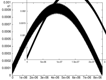
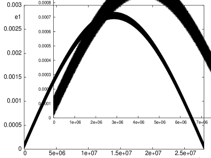
Figure 3: Inner eccentricity against time. Left column graphs: ${K_{1}=0.3}$, ${K_{2}=0.09}$, ${X=10}$ and ${\phi=90^{\circ}}$. Right column graphs: ${K_{1}=0.4}$, ${K_{2}=0.065}$, ${X=50}$ and ${\phi=90^{\circ}}$.The top graphs come from the numerical integration of the full equations of motion, the middle graphs show our theoretical solution based on the secular solution of Georgakarakos (2002) and the bottom graphs are based on the new secular solution.

Regarding the new secular solution we derived in subsection (2.2), it appears that we have achieved our aim, i.e. to correct the problem that arose from the singularity ${A-B=0}$ in the old solution. For example, if one checks the corresponding table in Georgakarakos (2006), he sees that for ${K_{1}=0.05}$ and ${K_{2}=0.01}$, the errors for ${X=10,20,30,50}$ are ${-1.7,-15.9,-17,-37}$ respectively. Using our new formula, the corresponding errors become ${9.4,3.9,3,1.6}$. Figures 3 demonstrate the improvement that is achieved by the use of our new formula. Both column graphs are plots of inner eccentricity against time. The left column graphs are for a system with ${K_{1}=0.3}$, ${K_{2}=0.09}$, ${X=10}$ and ${\phi=90^{\circ}}$, while the parameter values for the right column graphs are ${K_{1}=0.4}$, ${K_{2}=0.065}$, ${X=50}$ and ${\phi=90^{\circ}}$. The top graphs come from the numerical integration of the full equations of motion, the middle graphs are based on the old theoretical solution of Georgakarakos (2002) and the bottom graphs are produced by our new equations. The improvement is clearly noted (period and amplitude of oscillation). Note that, although ${X=50}$ for the right column graphs, and one may expect not to have a significant error, the old equations fail badly.

Finally, we would like to mention here, that , after a more careful inspection of the systems in Table 1 of Georgakarakos (2006), a few secular periods were corrected and some other systems that were not given a secular period, they now have one, as it can be seen in Table 1 of this paper.

Table 1: Percentage error between the averaged numerical ${e^{2}_{1}}$ and equation (18). For each (${K1,K2}$) pair, there are four entries, corresponding, from top to bottom, to ${X=10,20,30,50}$ respectively. The numbers in parentheses are the secular periods of the systems. In the system of units used, the inner binary period is ${T_{{\rm in}}=2\pi}$.

${K2\backslash\ K1}$	${0.001}$	${0.005}$	${0.01}$	${0.05}$	${0.1}$	${0.3}$	${0.5}$
0.001	11.9 (${1.15\times 10^{6}}$)	9.9 (${4.7\times 10^{5}}$)	9.2 (${2\times 10^{5}}$)	9.5 (${3.5\times 10^{4}}$)	9.8 (${1.9\times 10^{4}}$)	11 (${7.5\times 10^{3}}$)	12.2
	3 (${5\times 10^{6}}$)	1.8 (${3.5\times 10^{6}}$)	4.3 (${1.1\times 10^{6}}$)	3.1 (${1.9\times 10^{5}}$)	3.1 (${10^{5}}$)	3.3 (${4.2\times 10^{4}}$)	3.7
	2.4 (${1.05\times 10^{7}}$)	3.7(${1.05\times 10^{7}}$)	4.1 (${3\times 10^{6}}$)	1.8 (${5\times 10^{5}}$)	1.7 (${2.6\times 10^{5}}$)	1.7 (${1.1\times 10^{5}}$)	1.9
	-0.5 (${3\times 10^{7}}$)	2 (${5\times 10^{7}}$)	1.1 (${1.2\times 10^{7}}$)	0.9 (${1.7\times 10^{6}}$)	0.9 (${8.5\times 10^{5}}$)	0.8 (${3.7\times 10^{5}}$)	0.8
0.005	11.4 (${1.65\times 10^{5}}$)	12.8 (${2.2\times 10^{5}}$)	10.7 (${3\times 10^{5}}$)	9.6 (${4.2\times 10^{4}}$)	9.8 (${2.1\times 10^{4}}$)	11 (${8.5\times 10^{3}}$)	12.2
	4 (${6.45\times 10^{5}}$)	5.9 (${9\times 10^{5}}$)	5.8 (${1.6\times 10^{6}}$)	3.3 (${2.5\times 10^{5}}$)	3.1 (${1.15\times 10^{5}}$)	3.4 (${4.4\times 10^{4}}$)	3.7
	2.3 (${1.5\times 10^{6}}$)	3.8 (${2\times 10^{6}}$)	3.4 (${3.5\times 10^{6}}$)	1.3 (${7.2\times 10^{5}}$)	2 (${3\times 10^{5}}$)	1.8 (${1.15\times 10^{5}}$)	1.9
	1.1(${4.3\times 10^{6}}$)	1.8 (${5.5\times 10^{6}}$)	1.4 (${8.6\times 10^{6}}$	-0.5 (${2.7\times 10^{6}}$)	1.4 (${1.03\times 10^{6}}$)	0.8 (${4\times 10^{5}}$)	0.8
0.01	11.4 (${8\times 10^{4}}$)	11.1 (${10^{5}}$)	11 (${1.2\times 10^{5}}$)	9.4 (${5.6\times 10^{4}}$)	10 (${2.3\times 10^{4}}$)	11 (${9\times 10^{3}}$)	12.2
	4 (${3\times 10^{5}}$)	4.7 (${3.6\times 10^{5}}$)	3.2 (${5\times 10^{5}}$)	3.9 (${3.8\times 10^{5}}$)	4.3 (${1.3\times 10^{5}}$)	3.4 (${5\times 10^{4}}$)	3.8
	2.1 (${7.8\times 10^{5}}$)	3.1 (${8\times 10^{5}}$)	1.4 (${1.1\times 10^{6}}$)	3 (${1.22\times 10^{6}}$)	2.9 (${3.7\times 10^{5}}$)	1.5 (${1.45\times 10^{5}}$)	1.9
	1.2 (${2\times 10^{6}}$)	0.7 (${2.5\times 10^{6}}$)	1.4 (${2.8\times 10^{6}}$)	1.6(${6\times 10^{6}}$)	-0.9 (${1.5\times 10^{6}}$)	0.9 (${4.4\times 10^{5}}$)	0.8
0.05	12.5	12.5 (${1.4\times 10^{4}}$)	12.6 (${1.5\times 10^{4}}$)	12.3 (${2.2\times 10^{4}}$)	9.2 (${3.5\times 10^{4}}$)	12.2 (${1.8\times 10^{4}}$)	12.5
	4.4	4.6 (${6.5\times 10^{4}}$)	4.5 (${7\times 10^{4}}$)	6.3 (${9\times 10^{4}}$)	4.5 (${1.6\times 10^{5}}$)	5.4 (${1.2\times 10^{5}}$)	3.9
	2.4	2.8 (${1.45\times 10^{5}}$)	2.9 (${1.5\times 10^{5}}$)	4.4 (${2\times 10^{5}}$)	2.5 (${3.4\times 10^{5}}$)	2.8 (${4.2\times 10^{5}}$)	2
	1.1	1.3 (${4.6\times 10^{5}}$)	1.3 (${4.7\times 10^{5}}$)	1.7 (${5.7\times 10^{5}}$)	2.2 (${8.2\times 10^{5}}$)	1.8(${2.6\times 10^{6}}$)	0.9
0.1	13.9	13.5(${7\times 10^{3}}$)	13.2(${9\times 10^{3}}$)	13 (${9\times 10^{3}}$)	12.2 (${1.1\times 10^{4}}$)	-3 (${3.3\times 10^{4}}$)	12.8
	5.4	5.3 (${3.4\times 10^{4}}$)	5.4 (${3.2\times 10^{4}}$)	5.2 (${4\times 10^{4}}$)	4.5 (${5\times 10^{4}}$)	2.2 (${1.25\times 10^{5}}$)	4
	3.3	3.2(${7.9\times 10^{4}}$)	3 (${9\times 10^{4}}$)	3.4 (${9\times 10^{4}}$)	3 (${1.1\times 10^{5}}$)	2.4 (${2.35\times 10^{5}}$)	2.1
	1.8	1.8 (${2.2\times 10^{5}}$)	1.8 (${2.25\times 10^{5}}$)	2 (${2.5\times 10^{5}}$)	1.5 (${3\times 10^{5}}$)	2.1 (${5.2\times 10^{5}}$)	1
0.5	21.3	21.2	21	19.1 (${1.5\times 10^{3}}$)	18.3 (${1.5\times 10^{3}}$)	15.5(${1.8\times 10^{3}}$)	15
	10.1	9.9	9.7	8.9 (${8.5\times 10^{3}}$)	8.4 (${8.5\times 10^{3}}$)	6.4 (${8\times 10^{3}}$)	5.1
	6.8	6.7	6.5	5.9 (${2\times 10^{4}}$)	5.6 (${2\times 10^{4}}$)	3.9 (${2.2\times 10^{4}}$)	2.8
	4.2	4.1	3.9	3.8 (${5.7\times 10^{4}}$)	3.7 (${5.7\times 10^{4}}$)	2.7 (${6.5\times 10^{4}}$)	1.3
1	26.7	26.6	26.4	25	23.5	18.9	17.3
	12.8	12.7	12.6	11.5	10.4(${5\times 10^{3}}$)	7.3 (${5\times 10^{3}}$)	5.9
	8.8	8.7	8.6	7.7 (${1.2\times 10^{4}}$)	6.8 (${1.5\times 10^{4}}$)	4.5 (${1.3\times 10{4}}$)	3.2
	5.6	5.5	5.4	4.9 (${2.7\times 10^{4}}$)	4.3 (${4.5\times 10^{4}}$)	2.6 (${4.2\times 10^{4}}$)	1.6
3	34.2	34.1	33.9	32.5	28.2 (${1.3\times 10^{3}}$)	23.2 (${10^{4}}$)	22.2
	15.6	15.5	15.3	14.5	13.1	9	7.4
	10.7	10.6	10.5	9.8	8.7	5.4	4
	6.9	6.8	6.8	6.4	5.4	3	2
5	35.8	35.7	35.5	34.1	32.3	26.5	24.3
	15.6	15.6	15.4	14.5	13.3	9.4	7.9
	10.6	10.5	10.4	9.7	8.7	5.6	4.3
	6.8	6.8	6.7	6.3	5.5	3.1	2.1
10	36	35.9	35.7	34.5	32.9	28.1	26.2
	14.8	14.7	14.6	13.8	12.8	9.6	8.4
	9.8	9.7	9.6	8.9	8.2	5.6	4.6
	6.2	6.2	6.1	5.6	5.4	3.1	2.2
50	32.7	32.7	32.6	31.9	31.2	28.9	28.1
	11.8	11.8	11.7	11.3	10.8	9.4	8.9
	7.2	7.2	7.2	6.8	6.4	5.2	4.8
	4.3	4.3	4.2	4	3.7	2.7	2.4
100	31.4	31.4	31.4	30.9	30.4	28.9	28.3
	10.9	10.8	10.8	10.5	10.2	9.2	8.9
	6.5	6.4	6.4	6.2	5.9	5.1	4.8
	3.7	3.7	3.6	3.5	3.2	2.6	2.3
500	29.7	29.6	29.6	29.5	29.3	28.7	28.5
	9.6	9.6	9.6	9.5	9.4	9.1	8.9
	5.4	5.4	5.4	5.3	5.2	4.9	4.8
	2.9	2.9	2.9	2.8	2.7	2.5	2.4
1000	29.3	29.4	29.2	29.1	29	28.7	28.5
	9.4	9.4	9.4	9.3	9.2	9	8.9
	5.2	5.2	5.2	5.2	5.1	4.9	4.8
	2.7	2.7	2.7	2.6	2.6	2.4	2.4

4 SUMMARY

An even distant or light companion is expected to inject eccentricity to a close binary. A slight change in the binary separation can have drastic consequences on its subsequent evolution. Therefore, it is very useful to obtain analytical expressions about the amount of eccentricity injected into the binary orbit and the time-scales on which it is done. In addition, the analytical expressions could also be used for other purposes, such as the detection of a companion to a binary system (Mazeh and Shaham 1979), the determination of orbital elements of stellar triples or to set constrains to the masses and orbital elements of exoplanets.

In a series of papers, we derived formulae for estimating the inner eccentricity in hierarchical triple systems with various orbital characteristics and with the inner eccentricity being initially zero. The secular part of the solution we obtained in those papers, failed for certain combinations of the masses and the orbital parameters of some systems. In the current paper, we managed to obtain a secular solution for the inner eccentricity that had no such weakness. However the derivation applies only to hierarchical triple systems with initially circular outer binaries. For non-circular outer binaries, the system of the approximate secular differential equations is non-linear and therefore we can not obtain an improved solution as we did for the circular case. The numerical integrations of the full equations of motion confirmed that our new model works well where the previous one failed to do so.

Our future aim is to see whether a similar solution can be obtained for the non-coplanar formula of Georgakarakos (2004).

REFERENCES

Blaes O., Lee M. H., Socrates A., 2002, ApJ, 578, 775
Eggleton P., 2006, Evolutionary Processes in Binary and Multiple Stars. Cambridge University Press, UK
Eggleton P. P., Kiseleva L. G., 1996, in Wijers R. A. M. J., Davies M. B., eds, Proc. NATO Adv. Study Inst., Evolutionary Processes in Binary Stars. Kluwer Dordrecht, p. 345
Fekel F. C., Jr.; Tomkin J., 1982, ApJ 263, 289
Ford E. B., Kozinsky B., Rasio F. A., 2000, ApJ, 535, 385
Georgakarakos N., 2002, MNRAS, 337, 559
Georgakarakos N., 2003, MNRAS, 345, 340
Georgakarakos N., 2004, CeMDA, 89, 63
Georgakarakos N., 2006, MNRAS, 366, 566
Hinkle K. H., Fekel F. C., Johnson D. S., Scharlach W. W. G., 1993, AJ, 105, 1074
Jha S., Torres G., Stefanik R. P., Latham D. W., Mazeh T., 2000, MNRAS, 317, 375
Kiseleva-Eggleton L.G., Eggleton P.P., 2001, in Podsiadlowski P., Rappaport S., King A. R., D’Antona F., Burderi L., eds, ASP Conf. Ser. Vol 229, Evolution of Binary and Multiple Star Systems. Astron. Soc. Pac., San Francisco, p. 91
Kiseleva L. G., Eggleton P. P., Mikkola S., 1998, MNRAS, 300, 292
Krymolowski Y., Mazeh T., 1999, MNRAS, 304, 720
Libert A., Henrard J., 2005, CeMDA, 93, 187
Marchal C., 1990, The Three-Body Problem. Elsevier Science Publishers, the Netherlands
Mazeh T., 2008, in Goupil M.-J., Zahn J.-P., eds, EAS Publ. Ser. Vol 29, Tidal Effects in Stars, Planets and Disks, p. 1
Mazeh T.,Shaham J., 1979, A ${\&}$ A, 77, 145
Migaszewski C., Gozdziewski K., 2008, MNRAS, 388, 789
Mikkola S., 1997, CeMDA, 67, 145
Lee M. H., Peale S. J., 2003, ApJ 592, 1201
Tokovinin A.A., 1997, A ${\&}$ AS, 124, 75