A signature for the Luttinger liquid phase in alternating Heisenberg spin-1/2 chains

Abstract

We have studied the zero and low-temperature behavior of anisotropic alternating antiferromagnetic-ferromagnetic Heisenberg spin-1/2 chains in a transverse magnetic field. Using the analytical spinless fermion approach, the thermodynamic behavior of the model has been studied. We have introduced a new order parameter to distinguish the gapless Luttinger liquid phase from the other gapped phases. The exact diagonalization Lanczos results are also used to compare with the spinless fermion ones. We have found a double peak structure in the specific heat curves for the region between the two quantum critical points. Using the numerical full diagonalization results, the existence of the double peak structure is confirmed.

I introduction

The study of continuous phase transitions has been one of the most fertile branches of theoretical physics in the last decades. Each phase can usually be characterized by an order parameter. Often, the choice of an order parameter is obvious. However, in some cases finding an appropriate order parameter is complicated. In particular, many magnetic systems experience the Luttinger liquid (LL) phase for certain values of some non-thermal control parameter. Luttinger liquid is the paradigm for the description of interacting one-dimensional (1D) quantum systemsGiam04 ; Taka99 . The correlation functions decay as power laws and the ground state has a quasi-long range order. In spite of all manifestations of this phase, the magnetic ordering in the LL phase is still unclear, i.e, all suggested local magnetic order parameters turn out to be zero, having no effect in determining the structure of the LL phase. In this work, we will concentrate on studying the probably nonlocal magnetic ordering of the LL phase.

One dimensional quantum spin systems such as antiferromagnetic spin-1/2 chainsLake05 , spin ladder systemsDago96 , or bond alternating spin-1/2 AF-F chains are good candidates for studying the LL phase. When these systems are placed in an external magnetic field, they can be mapped onto a 1D system of interacting spinless fermionsGiam04 ; Chit97 ; Usam98 ; Furu99 ; Hiki01 ; Yama05 . The filling of a fermionic band can thus be continuously tuned, making these systems suitable for probing the LL physicsGiam04 ; Lake05 ; Okun07 ; Kimu08 . In the case of isotropic bond alternating AF-F spin-1/2 chains the whole band can be covered. In the absence of an external magnetic field ($h=0$), the model is mapped onto a nonlinear sigma model with a $4\pi s$ topological angleBosq00 . This model is always gapful and can be regarded as a Haldane gapped spin-1 chainHald83 . The gap decreases by increasing the magnetic field and goes to zero at the lower critical field $h_{c_{1}}$Mahd1-08 . At $h_{c_{1}}$, the system enters the gapless phase and the fermionic band starts to be filled. This process continues until the upper critical field $h_{c_{2}}$ is reached. Increasing the field beyond $h_{c_{2}}$ reopens the gap and the band is then completely filled.

Recently, It was demonstrated that ${\rm CuBr_{4}(C_{5}H_{12}N)_{2}}$ is a unique system for controlling and probing the physics of LL Klan08 . This sample is a spin ladder system with $h_{c_{1}}=6.6$ T and $h_{c_{2}}=14.6$ TWats01 . Bond alternating AF-F spin-1/2 chains that allow experimental access to the whole fermionic band are not known. However the $\rm{(CH_{3})_{2}NH_{2}CuCl_{3}}$ system has been considered to be a suitable realization of bond alternating AF-F spin chain. Linked-cluster calculations and bulk measurements show that $\rm{DMACuCl_{3}}$ is also a realization of the spin-1/2 alternating AF-F chain with nearly the same strength of antiferromagnetic and ferromagnetic couplingsSton07 . Other experimental samples of the AF-F alternating spin-1/2 chain compounds have also been reported in Refs.[Hagi97, ; Taka97, ; Koda99, ; Mana97-1, ; Mana97-2, ]. Although it is not known whether these systems can experience the LL phase, theoretically, an isotropic bond alternating AF-F spin chain, in its ground state, can enter the LL phase with quasi-long range order. In this paper, we look for an order parameter to describe the LL phase of the bond alternating AF-F spin-1/2 chain. The Hamiltonian of this model with anisotropic ferromagnetic coupling is given by

$$\hat{H} = -J_{F}\sum_{j=1}^{N/2}(S_{2j}^{x}S_{2j+1}^{x}+\Delta S_{2j}^{y}S_{2j+1}^{y}+S_{2j}^{z}S_{2j+1}^{z})$$ (1)

$$+J_{AF}\sum_{j=1}^{N/2}{\bf S}_{2j-1}\cdot{\bf S}_{2j}+h\sum_{j=1}^{N}S_{j}^{\alpha},$$

where $S_{j}^{\alpha},(\alpha=x,y,z)$ are spin-1/2 operators on the $j$-th site. $J_{F}$ and $J_{AF}$ denote the ferromagnetic and antiferromagnetic couplings, respectively. $\Delta$ is the anisotropy parameter and $h$ is a uniform magnetic field.

The ground-state propertiesTaka92 ; Hida92a ; Hida93 ; Saka95 ; Hida92b ; Kohm92 ; Yama93 and low-lying excitationsHida94 of this model have been thoroughly investigated by numerical tools and variational schemes. In particular, the string order parameter which was originally defined for the spin-1 Heisenberg chainsNijs89 has been generalized to this system. The ground state has long-range string order, which is characteristic of the Haldane phase. Hida has shown that the Haldane phase of the AF-F alternating chain is stable against any strength of randomnessHida99 . The ground state phase diagram of the AF-F alternating chain in a longitudinal ($\alpha=y$) magnetic field is studied using numerical diagonalization and finite-size scaling based on conformal field theorySaka95 . It is shown that the magnetic state is gapless and described by the LL phase. The model represented by the Hamiltonian in Eq. 1 which includes a transverse magnetic field has been studied recently using the numerical Lanczos methodMahd1-08 . The main attention in this study was focused on the investigation of field-induced effects in the ground state phase diagram, present when the antiferromagnetic coupling $J_{AF}$ dominates ($J_{AF}>J_{F}$). The system has two critical fields and the energy gap in the intermediate region depends on the anisotropic parameter $\Delta$. For $\Delta\neq 1$, the intermediate state is gapful and the ground state of the model has stripe-antiferromagnetic orderMahd1-08 .

In this paper we consider again an anisotropic AF-F chain in a transverse magnetic field. Using the numerical exact diagonalization method and the analytical spinless fermion approach, we investigate the zero temperature and thermodynamic behavior of the model. We introduce a new mean field order parameter which can distinguish the LL phase from the other gapped phases (Fig. 2). In the specific heat curves versus temperature, a double peak structure appears in the intermediate region of the magnetic fields $h_{c_{1}}<h<h_{c_{2}}$.

The outline of the paper is as follows. In section II we discuss the zero-temperature ground state phase diagram of the model. In section III we present the results of the spinless fermion approach and the numerical full diagonalization results on the low-temperature behavior of the model. Finally we conclude and summarize our results in section IV.

II zero-temperature behavior

II.1 RESULTS FROM THE NUMERICAL LANCZOS METHOD

In this section we briefly discuss the model (1) in the limiting case of the strong AF coupling $J_{AF}\gg J_{F}$. In this limit the model can be mapped onto an effective spin-chain HamiltonianMila98 . At $J_{AF}\gg J_{F}$, the system behaves as a nearly independent block of pairsMila98 . Indeed an individual block may be in a singlet or a triplet state with the corresponding energies given by

$$E_{1,-1}={J_{AF}\over 4}\ \mp h,\,\,E_{0}={J_{AF}\over 4},\,\,E_{s}=-{3J_{AF}\over 4}.$$

For $h\leq J_{AF}$, one component of the triplet becomes closer to the singlet ground state such that for a strong enough magnetic field we have a situation when the singlet and $S^{z}=1$ component of the triplet create a new effective spin $\tau=1/2$ system. On the new singlet-triplet subspace, the original Hamiltonian becomes the Hamiltonian of a fully anisotropic XYZ spin-1/2 chain in an effective magnetic fieldMahd1-08

$$H_{\emph{eff}} = \frac{J_{F}}{2}\sum_{j=1}^{N/2}[-\frac{1}{2}\tau^{z}_{j}\tau^{z}_{j+1}+\Delta\tau^{y}_{j}\tau^{y}_{j+1}+\tau^{x}_{j}\tau^{x}_{j+1}]$$ (2)

$$+ h^{eff}\sum_{j=1}^{N/2}\tau^{z}_{j}\,,$$

where $\mathrm{h}^{eff}=h-J_{AF}+J_{F}/4$. At $\Delta=1$, the effective problem reduces to the theory of the $XXZ$ chain with a fixed antiferromagnetic anisotropy of $1/2$ in a magnetic fieldTaka99 . The gapped Haldane phase at $\mathrm{h}^{eff}<\mathrm{h}^{eff}_{c_{1}}=-\frac{J_{F}}{4}$ for the AF-F alternating chain corresponds to the negatively saturated magnetization phase for the effective spin chain, whereas the massless LL phase of the AF-F alternating chain corresponds to the finite magnetization phase of the effective spin-1/2 chain. The critical field $\mathrm{h}^{eff}_{c_{2}}=\frac{J_{F}}{4}$ where the AF-F alternating chain is totally magnetized, corresponds to the fully magnetized phase of the effective spin chain.

Away from the isotropic point $\Delta=1$ the effective Hamiltonian (2) describes the fully anisotropic ferromagnetic XYZ chain in a magnetic field that is directed perpendicular to the easy axis. In this case, it is foundMahd1-08 that a gapped stripe-antiferromagnetic phase exists for the intermediate values of the transverse magnetic field $h_{c_{1}}<h<h_{c_{2}}$.

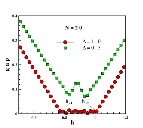
To recognize the different phases induced by the transverse magnetic field in the ground-state phase diagram, we implemented the modified Lanczos algorithm of finite-size chains $(N=12,16,20,24)$Mahd1-08 with $J_{AF}=1,J_{F}=1/2$ and different values of the anisotropy parameter $\Delta$. The energies of a few lowest eigenstates were obtained for the chains with periodic boundary conditions. In Fig. 1 we have plotted the results of these calculations for different values of the anisotropy parameter $\Delta=1.0,~{}0.5$, and chain length $N=20$. As it is clearly seen from this figure, in the case of zero magnetic field the spectrum of the model is gapped. For $h\neq 0$ the gap decreases linearly with $h$ and vanishes at the critical field $h_{c_{1}}(\Delta)$. In the isotropic case $\Delta=1.0$, the spectrum remains gapless for $h_{c_{1}}=0.78\pm 0.01<h<h_{c_{2}}=1.0$ and becomes once again gapped for $h>h_{c_{2}}$. But, in the anisotropic case $\Delta=0.5$, the excitation spectrum is gapfull except at two critical field values $h_{c_{1}}=0.82\pm 0.01$ and $h_{c_{2}}=0.94\pm 0.01$. In the intermediate region $h_{c_{1}}<h<h_{c_{2}}$ the spin gap which appears at $h>h_{c_{1}}$, first increases vs external field and after passing a maximum decreases to vanish at $h_{c_{2}}$.

In conclusion, at $T=0$, two quantum phase transitions in the ground-state phase diagram of the model have been identified with increasing transverse magnetic field Mahd1-08 . The first transition corresponds to the transition from the gapped Haldane phase to the gapless LL phase (or gapped stripe-antiferromagnetic for the anisotropic case). The other one is the transition from the gapless LL phase (or gapped stripe-antiferromagnetic) to the fully polarized phase.

Figure 1: The excitation gap of a spin-1/2 AF-F chain versus the uniform magnetic field $h$, for different anisotropy parameters $\Delta=1.0,~{}0.5$ and chain size $N=20$.

II.2 FERMIONIZATION

The behavior of the gap and the quantum phase space of the model lead us to investigate the thermodynamic properties of the model. In this respect, we implement the Jordan-Wigner transformation to fermionize the model. Because of two types of coupling constant, we introduce two kinds of spinless fermion through the following Jordan-Wigner transformations:

$$S_{2n-1}^{+} = a_{n}^{\dagger}e^{i\pi\bigg{(}\sum_{m=1}^{n-1}a_{m}^{\dagger}a_{m}+\sum_{m=1}^{n-1}b_{m}^{\dagger}b_{m}\bigg{)}},$$

$$S_{2n}^{+} = b_{n}^{\dagger}e^{i\pi\bigg{(}\sum_{m=1}^{n}a_{m}^{\dagger}a_{m}+\sum_{m=1}^{n-1}b_{m}^{\dagger}b_{m}\bigg{)}},$$

$$S_{2n-1}^{z} = a_{n}^{\dagger}a_{n}-\frac{1}{2},~{}~{}~{}~{}~{}~{}~{}S_{2n}^{z}=b_{n}^{\dagger}b_{n}-\frac{1}{2}.$$

Using the above transformations, the thermodynamic behavior of the isotropic ($\Delta=1$) Heisenberg AF-F spin-1/2 chains has been studied in the absence of a magnetic fieldYama05 . By the above transformations, the AF-F spin chain is mapped onto a 1D system of interacting spinless fermions;

$$\hat{H}_{f} = -\frac{Nh}{2}+\sum_{n=1}^{N/2}(\frac{J_{F}}{2}-\frac{J_{AF}}{2}+h)(a_{n}^{\dagger}a_{n}+b_{n}^{\dagger}b_{n})$$ (3)

$$+\sum_{n=1}^{N/2}(\frac{J_{AF}}{2}a_{n}^{\dagger}b_{n}-\frac{1+\Delta}{4}J_{F}a_{n+1}^{\dagger}b_{n}$$

$$-\frac{1-\Delta}{4}J_{F}b_{n}^{\dagger}a_{n+1}^{\dagger}+h.c)+\sum_{n=1}^{N/2}J_{AF}a_{n}^{\dagger}a_{n}b_{n}^{\dagger}b_{n}$$

$$-\sum_{n=1}^{N/2}J_{F}b_{n}^{\dagger}b_{n}a_{n+1}^{\dagger}a_{n+1}.$$

Treating the Hamiltonian $H_{f}$ in the mean field approximation, the interacting fermionic system reduces to a 1D system of new non-interacting dynamical quasi-particles. Many mean field order parameters (auxiliary fields) might be considered. Many of them are irrelevant, i.e., they do not have a stable mean field solution, while some are relevant. In our system we have introduced the magnetization, ferromagnetic and antiferromagnetic dimers as mean field order parameters;

$$\langle a_{n}^{\dagger}a_{n}\rangle = d_{a},~{}~{}~{}\langle b_{n}^{\dagger}b_{n}\rangle=d_{b},$$ (4)

$$\langle a_{n+1}^{\dagger}b_{n}\rangle = P_{F},~{}~{}\langle b_{n}^{\dagger}a_{n}\rangle=P_{AF}.$$

Utilizing the above order parameters, the mean field Hamiltonian is given by;

$${\cal H}_{HF}=E_{0}+\sum_{k}{\frac{A}{2}a_{k}^{\dagger}a_{k}+\frac{B}{2}b_{k}^{\dagger}b_{k}+\gamma_{k}a_{k}^{\dagger}b_{k}+h.c}$$ (5)

where,

$$A = (J_{AF}-J_{F})(d_{b}-1/2)+h,$$

$$B = (J_{AF}-J_{F})(d_{a}-1/2)+h,$$

$$\gamma_{k} = J_{AF}(1/2-P_{AF})e^{ik/2}+J_{F}(P_{F}^{*}-\frac{1+\Delta}{4})e^{-ik/2}$$

$$E_{0} = \frac{N}{2}\bigg{(}J_{AF}(|P_{AF}|^{2}-d_{a}d_{b}+1/4)-h$$ (6)

$$-J_{F}(|P_{F}|^{2}-d_{a}d_{b}+1/4)-\frac{J_{F}}{16}(1-\Delta^{2})^{2}\bigg{)}.$$

In the above, $\langle\dots\rangle$ represents thermal averaging over the Hartree-Fock eigen-states. $d_{a}$ and $d_{b}$ are related to the magnetization, and $P_{F}$ and $P_{AF}$ are ferromagnetic and antiferromagnetic exchange order parameters, respectively. It is clear that $P_{AF}(P_{F})$ in the Hilbert space is the AF(F)-dimer order parameter, i.e.,

$$\langle S^{-}_{2n}S^{+}_{2n+1}\rangle=\langle a_{n+1}^{\dagger}b_{n}\rangle=P_{F},$$

$$\langle S^{-}_{2n-1}S^{+}_{2n}\rangle=\langle b_{n}^{\dagger}a_{n}\rangle=P_{AF}.$$ (7)

Using the following unitary transformations

$$a_{k} = u_{k}\alpha_{k}+v_{k}e^{i\theta_{k}}\beta_{k},$$

$$b_{k} = v_{k}e^{-i\theta_{k}}\alpha_{k}+u_{k}\beta_{k},$$

the diagonalized Hamiltonian is given by

$${\cal H} = E_{0}+\sum_{k}\sum_{\sigma=\pm}(\epsilon_{k}^{+}\alpha^{\dagger}\alpha_{k}+\epsilon_{k}^{-}\beta^{\dagger}\beta_{k}),$$

$$\epsilon_{k}^{\pm}=\xi\pm\sqrt{\eta^{2}+\gamma_{k}^{2}}+h,$$

$$\eta=\frac{B-A}{2},~{}~{}~{}~{}~{}~{}\xi=\frac{B+A}{2},$$

Equation(6) clearly shows that the effect of the anisotropy appears in the dispersion relations. The dispersion relations of low-lying excitation read as,

$$\epsilon_{k}^{\pm}\cong\pm[(J_{AF}\tilde{P}_{AF}-J_{F}\tilde{P}_{F})^{2}+J_{AF}J_{F}\tilde{P}_{AF}\tilde{P}_{F}k^{2}]^{\frac{1}{2}}+h,$$

where $\tilde{P}_{AF}=1/2-ReP_{AF}$ and $\tilde{P}_{F}=\frac{1+\Delta}{4}-ReP_{F}$. Using the above order parameters, the thermodynamic functions such as the internal energy and the specific heat are expressed as follows:

$$U = E_{0}+\sum_{k}\sum_{\sigma=\pm}\epsilon_{k}^{\sigma}\bar{n}_{k}^{\sigma},$$

$$C = \frac{\partial U}{\partial T},$$ (10)

where, $\bar{n}_{k}^{\sigma}=[e^{\frac{\epsilon_{k}^{\sigma}}{T}}+1]^{-1}$ is the fermion distribution function (choose $k_{\rm B}=1$).

In order to obtain the thermodynamic behavior of the system, we need to know the whole temperature behavior of the order parameters for different values of $h$. The order parameters satisfy a set of self consistent equations and it should be solved the equations (4), self-consistently.

In Fig.2-(a), we have plotted the ferromagnetic dimer order parameter of both anisotropic $(\Delta=0.5)$ and isotropic ($\Delta=1$) AF-F Heisenberg spin-1/2 chains versus $h$. The curves have been plotted close to the zero temperature. As we mentioned, at $T=0$ for different values of $h$, our 1D system experiences three phases. In the Haldane phase ($h<h_{c_{1}}$), the quantum fluctuations are strong enough to suppress the ferromagnetic order of the system and the AF(F)-dimer parameters $P_{AF}(P_{F})$ should be close to the classical value $-0.5(0)$Japa07 . In this region the energy spectrum is gapped and the gap is decreased by increasing $h$.

Figure 2: a) The spinless fermion results of the real part of the ferromagnetic exchange order parameter at temperature $T=0.05$ versus $h$, $J_{AF}=1$ and $J_{F}=0.5$, b) Exact diagonalization Lanczos results of the real part of the $P_{F}$ for a chain size $N=20$.

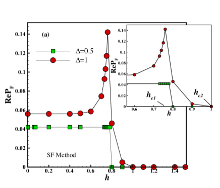
The first quantum phase transition occurs at $h_{c_{1}}$. At the same time the fermionic band starts to be filled where the excited state sticks to the ground state and the gap of the system is closed. For the first region there is no specific difference between the two anisotropic and isotropic cases. i.e., anisotropy shows a marked behavior for the case of $h_{c_{1}}<h<h_{c_{2}}$.

For the case of $\Delta=1$ and $h=0$, the system is isotropic and has SU(2) rotational symmetry. In the intermediate region this system is gapless and correlations decay in a power lawSaka95 . In this region, the Luttinger liquid phase, the magnetic field suppresses quantum fluctuations and induces quasi long-range order in the 1D system. Although the power law behavior of the correlations and other properties of the LL phase are manifest, the lack of an order parameter to show the behavior of the system in this phase is still felt. As it is obviously seen from Fig.2, the F-dimer order parameter has a considerable value in this region and is sensitive to $h$. The value of this order parameter falls sharply at the second critical field where the fermionic band is completely filled and the gap of the system is reopened.

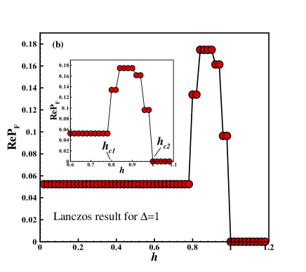
We have also plotted in Fig.2-(b) the F-dimer order parameter of the isotropic AF-F Heisenberg spin-1/2 chain by using the exact diagonalization Lanczos results. The numerical Lanczos method is implemented as a reference approach to see the accuracy of our spinless fermion method. As it is clearly observed from Fig.2-(b) the results of Lanczos method, confirms that the defined mean field order parameter has considerable value for the intermediate values of field.

We have also plotted in Fig.2 the F-dimer order parameter of anisotropic F-AF spin-1/2 chain versus transverse magnetic field. Regarding the anisotropy in ferromagnetic coupling, the anisotropic system is mapped to a 1D XYZ model with U(1) symmetry. In the intermediate region ($h_{c_{1}}<h<h_{c_{2}}$) the system has the magnetic long range order and spins are aligned stripe-antiferromagnetically. This phase is gapfull and the F-dimer order has no considerable value in the this phase. Moreover, there is a big discrepancy between the values of the F-dimers of the isotropic and anisotropic cases, i.e. in the LL gapless phase the behavior of the F-dimer order parameter ($ReP_{F}$) is different from those of the gapped phases. Therefore, we can conclude that the above F-dimer order parameter can distinguish between the gapless LL phase and the other gapped phases.

This means that experimenters might look for such behavior in $ReP_{F}$ at finite temperatures. I.e., experimental results on this quantity may be used to distinguish between the isotropic chains and anisotropic ones (gapped stripe-antiferromagnetic and gapless LL phases).

III Thermal behavior of the model

In this section we will study the thermal behavior of the mean field order parameters of the Heisenberg spin-1/2 AF-F chains in both anisotropic and isotropic cases. The order parameters also have different behavior for different values of $h$.

For $h<h_{c_{1}}$, in the Haldane phase, an increase in temperature increases the thermal fluctuations and Haldane ordering is suppressed. The solution of the Eqs. 4 shows that the AF-dimer order parameter ($ReP_{AF}$) decreases with temperature.

However, $J_{F}$ couplings supply an interaction between the unit cells and try to establish F-dimer order ($ReP_{F}$) even at moderate temperatures (scaled with $J_{F}$), i.e. ($ReP_{F}$) increases with temperature up to $T_{F}$ (see Fig. 3). Above $T_{F}$, fluctuations are large enough to decrease $ReP_{F}$. The locations of the maximum value of ($ReP_{F}$) with respect to $h$ are shown in Fig.3. As it is obviously seen from this plot, there is a peak at $h$ very close to the first critical field. The location of this peak is a good candidate to find the first critical point.

By increasing the magnetic field, the value of $T_{F}$ (location of the maximum value of $ReP_{F}$) decreases. It is found that $T_{F}$ goes to a minimum (Fig.4) when $h$ increases up to $h_{c_{1}}$. Increasing the magnetic field further and for $h_{c_{1}}\sim 0.76<h<h_{c_{2}}\sim 1$, $T_{F}$ always maintains a minimum value and the value of $ReP_{F}$ decreases monotonically with increasing $T$. Increasing the magnetic field even further, for $h>h_{c_{2}}$, $T_{F}$ also increases.

Figure 3: The spinless fermion results of the real part of the ferromagnetic exchange order parameter at temperature $T_{F}$ versus $h$, for $J_{AF}=1$ and $J_{F}=0.5$ .

Figure 4: The spinless fermion results for $T_{F}$ versus $h$, with $J_{AF}=1$ and $J_{F}=0.5$ .

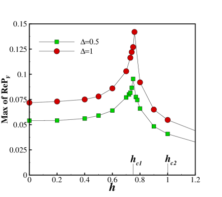
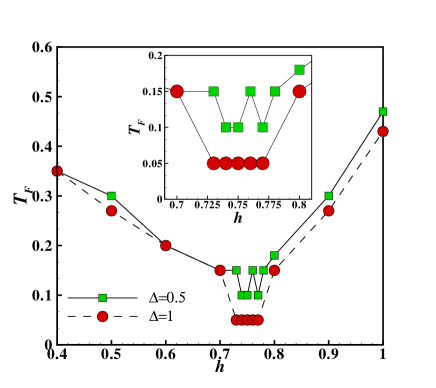
The SF calculations also show that the behavior of $T_{F}$ is similar to the energy gap (see Fig.1)

Figure 5: The spinless fermion results of the specific heat of an alternating AF-F spin-1/2 chain versus $T$ for different values of the magnetic field $h$ with $J_{AF}=1$ and $J_{F}=0.5$. (a) $\Delta=1$ (b) $\Delta=0.5$.

Figure 6: Full diagonalization results of the specific heat of an alternating AF-F spin-1/2 chain versus $T$ for different values of the magnetic field $h$ with $J_{AF}=1$ and $J_{F}=0.5$. (a) $\Delta=1$ (b) $\Delta=0.5$.

Figure 7: Specific heat of the AF-F Heisenberg spin-1/2 chain vs. $T$ for both values of $\Delta$ and $h=0.9$ using the spinless fermion (SF) and full diagonalization (FD) approaches.

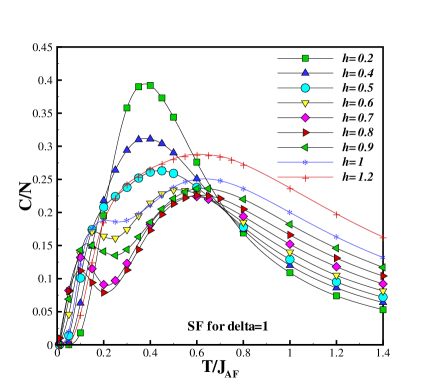
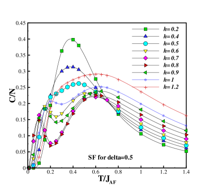
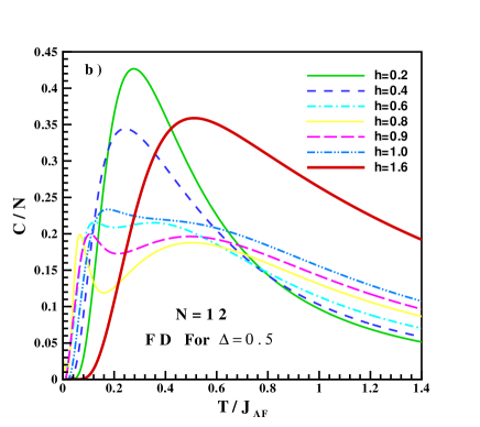
The discovery of gapless or gapped excitations have led to the investigation of the thermodynamic properties of the model. One of the most important thermodynamic functions is the specific heat. In this respect, we study the temperature-dependence of the specific heat of the model in different quantum regimes. We have calculated the specific heat of both isotropic and anisotropic cases, using two methods, the analytical SF and the numerical full diagonalization methods. In Fig. 5a(b) we have plotted the results of the SF method in the form of the specific heat $C/N$ versus $T$ with $\Delta=1$ and $\Delta=0.5$ for different values of $h$. As it is clearly seen from this figure, in the Haldane and paramagnetic regions ($h<h_{c_{1}}$ and $h>h_{c_{2}}$, respectively), there is only one peak on the specific heat curve. However, in the intermediate region ($h_{c_{1}}<h<h_{c_{2}}$) a double peak is observed. At $h=0$ there is a Schottky like peak in the specific heat which is expected from the Haldane phase. By increasing $h$, the peak becomes wider and goes to lower temperatures. Increasing $h$ further, causes a shoulder to appear on the right hand side of the curve. For $h>h_{c_{1}}$, increasing $h$, an additional peak appears which is the signal for the paramagnetic phase. Because of the two F and AF interactions ($J_{F}$ and $J_{AF}$), there are two kinds of quasi-particles in the system. These quasi-particles have two different dynamics. These dynamics bring about two energy scales in the system. The energy scales affect the behavior of the response functions. It is obviously seen from the plots of the specific heat $C/N$ that the energy scales create a double peak in the specific heat at two different temperatures. As a general statement, two energy scales can produce a double peak structure in the specific heat.

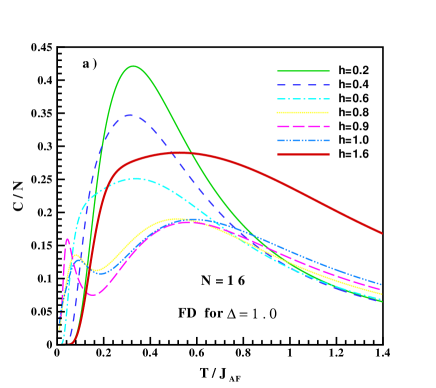
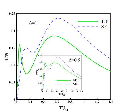
We have also plotted in Figs. 6 a(b) the specific heat of the model by using the full diagonalization method. We have computed all the eigenvalues of the energies for different values of the transverse magnetic field $h$ and anisotropy parameter $\Delta$. Therefore, using these eigen-energies, we have computed the specific heat as a function of the temperature $T$. The specific heat curves have been plotted for $J_{AF}=1$ and $J_{F}=0.5$ and the anisotropy parameter $a)\Delta=1$, $b)\Delta=0.5$. As it is clearly seen from this figures, in the Haldane and paramagnetic regions ($h<h_{c_{1}}$ and $h>h_{c_{2}}$, respectively), there is only one peak in the specific heat curve. To see the qualitative agreement between spinless fermion results and Full diagonalization ones, we have plotted the specific heat versus $T$ for an intermediate value of $h$ (for example $h=0.9$). As it is seen from Fig.7 the mean field results are in agreement with the others, qualitatively. It is interesting that the numerical results confirm the existence of the double peak in the intermediate region ($h_{c_{1}}<h<h_{c_{2}}$).

IV conclusion

To summarize, we have studied the zero and finite-temperature behavior of the anisotropic alternating AF-F Heisenberg spin-1/2 chains in a transverse magnetic field. The numerical exact diagonalization method and analytical spinless fermion approach are applied to analyze the model. The first notable point is introducing a new mean field order parameter which can distinguish between a gapless LL phase and the gapped phases. This order parameter in the spin language of Hilbert space is the F-dimer order parameter. In the isotropic case, the F-dimer order parameter has a considerable value in the LL region. We have shown that there is a big discrepancy between the values of the F-dimers of the isotropic and anisotropic cases, i.e., in the LL gapless phase the behavior of the F-dimer order parameter ($ReP_{F}$) is different from that of the gapped phases. Therefore, we have concluded that the F-dimer order parameter can distinguish the gapless LL phase from the other gapped phases.

The second notable point is found from the specific heat. We have obtained a double peak structure in the specific heat curves vs temperature.

There are some questions behind the defined order parameter which are still controversial and we can investigate them in future. The most remarkable questions referred to the topological order and spontaneous symmetry breaking. I.e. in the LL phase, where the real part of the F-dimer is not zero, how can describe topological order and what kind of spontaneous symmetry breaking is occurred.

V Acknowledgments

It is our pleasure to thank G. I. Japaridze for his valuable comments and fruitful discussions. J. A. also would like to thank A. Langari and F. Shahbazi for their useful suggestions and comments. We are also grateful to B. Farnudi for reading carefully the manuscript and appreciate his useful comments. J. A. was supported by the grant of Shahrood University of Technology.

References

- (1) T. Giamarchi, Quantum physics in one dimension, (Oxford Univ.Press, Oxford, 2004).
- (2) M. Takahashi, Thermodynamics of one-dimensional solvable models, (Cambridge University Press: Cambridge, 1999 ).
- (3) B. Lake, D. A. Tennant, C. D. Frost and S. E. Nagler, Nat. Mat. 4, 329 (2005).
- (4) E. Dagotto and T. M. Rice, Science 271, 618 (1996).
- (5) R. Chitra and T. Giamarchi, Phys. Rev. B 55, 5816 (1997).
- (6) M. Usami and S. Suga, Phys. Rev. B 58, 14401 (1998).
- (7) A. Furusaki and S.-C. Zhang, Phys. Rev. B 60, 1175 (1999).
- (8) T. Hikihara and A. Furusaki, Phys. Rev. B 63, 134438 (2001).
- (9) S. Yamamoto et. al,: Fiz. Nizk. Temp. 31, 974 (2005).
- (10) K. Okunishi and T. Suzuki, Phys. Rev. B 76, 224411 (2007).
- (11) S. Kimura, T. Takeuchi, K. Okunishi, M. Hagiwara, Z. He, K. Kindo, T. Taniyama and M. Itoh, Phys. Rev. Lett. 100 057202 (2008).
- (12) M. Bosquet and Th. Jolicoeur, Eur. Phys. J. B, 14, 47 (2000).
- (13) F. D. M. Haldane: Phys. Rev. Lett 50, 1153 (1983) .
- (14) S. Mahdavifar and A. Akbari, J. Phys. Soc. Jpn. 77, 024710 (2008).
- (15) M. Klanjek, H. Mayaffre, C. Berthier, M. Horvati, B. Chiari, O. Piovesana, P. Bouillot, C. Kollath, E. Orignac, R. Citro and T. Giamarchi, arXiv:0804.2639
- (16) B. C. Watson, et. al, Phys. Rev. Lett. 86 5168 (2001).
- (17) M. B. Stone, W. Tian, M. D. Lumsden, G. E. Granroth, D. Mandrus, J.-H. Chung, N. Harrison, and S. E. Nagler: Phys. Rev. Lett 99, 087204 (2007).
- (18) M. Hagiwara, Y. Narumi, K. Kindo, T. C. Kobayashi, H. Yamakage, K. Amaya, and G. Schumauch, J. Phys. Soc. Jpn. 66, 1792 (1997).
- (19) M. Takahashi, Y. Hosokoshi, H. Nakano, T. Goto, and M. Kinoshita: Mol. Cryst. Liq. Cryst. Sci. Technol., Sect. A 306, 111 (1997).
- (20) K. Kodama, H. Harashina, H. Sasaki, M. Kato, M. Sato, K. Kakurai, and M. Nishi: J. Phys. Soc. Jpn. 68, 237 (1999).
- (21) H. Manaka, I. Yamada and K. Yamaguchi, J. Phys. Soc. Jpn. 66, 564 (1997).
- (22) H. Manaka and I. Yamada, J. Phys. Soc. Jpn. 66, 1908 (1997).
- (23) S. Takada: J. Phys. Soc. Jpn. 61 (1992) 428.
- (24) K. Hida and S. Takada: J. Phys. Soc. Jpn. 61, 1879 (1992) .
- (25) K. Hida: J. Phys. Soc. Jpn. 62, 439 (1993).
- (26) T. Sakai: J. Phys. Soc. Jpn. 64, 251 (1995).
- (27) K. Hida: Phys. Rev. B 46, 8268 (1992).
- (28) M. Kohmoto and H. Tasaki: Phys. Rev. B 46, 3486 (1992).
- (29) M. Yamanaka, Y. Hatsugai, and M. Kohmoto: Phys. Rev. B 48, 9555 (1993).
- (30) K. Hida: J. Phys. Soc. Jpn. 63, 2514 (1994).
- (31) M. den Nijs and K. Rommelse: Phys. Rev. B 40 ,4709 (1989).
- (32) K. Hida: Phys. Rev. Lett 83 ,3297 (1999).
- (33) F. Mila, Eur. Phys. J. B 6, 201 (1998).
- (34) G. I. Japaridze, A. Langari, and S. Mahdavifar, J. Phys.: Condens. Matter 19, 076201 (2007).
- (35) S. Mahdavifar and A. Akbari, J. Phys.: Condens. Matter, 20, 215213 (2008).