Entanglement renormalization in two spatial dimensions
Abstract
We propose and test a scheme for entanglement renormalization capable of addressing large two-dimensional quantum lattice systems. In a translationally invariant system, the cost of simulations grows only as the logarithm of the lattice size; at a quantum critical point, the simulation cost becomes independent of the lattice size and infinite systems can be analysed. We demonstrate the performance of the scheme by investigating the low energy properties of the 2D quantum Ising model on a square lattice of linear size with periodic boundary conditions. We compute the ground state and evaluate local observables and two-point correlators. We also produce accurate estimates of the critical magnetic field and critical exponent . A calculation of the energy gap shows that it scales as at the critical point.
pacs:
05.30.-d, 02.70.-c, 03.67.Mn, 05.50.+qEntanglement renormalization ER has been recently proposed as a real-space renormalization group (RG) method Wilson to study extended quantum systems on a lattice. A highlight of the approach is the removal, before the coarse-graining step, of short-range entanglement by means of unitary transformations called disentanglers. This prevents the accumulation of short-range entanglement over successive RG transformations. Such accumulation is the reason why the density matrix renormalization group (DMRG) DMRG – an extremely powerful technique for lattices in one spatial dimension – breaks down in two dimensions, where it can only address small systems.
The use of disentanglers leads to a real-space RG transformation that can in principle be iterated indefinitely, enabling the study of very large systems in a quasi-exact way. This RG transformation also leads to the so-called multi-scale entanglement renormalization ansatz (MERA) MERA to describe the ground state of the system – or, more generally, a low energy sector of its Hilbert space. In a translation invariant lattice made of sites, the cost of simulations grows only as NewAlgorithm . In the presence of scale invariance, this additional symmetry is naturally incorporated into the MERA and a very concise description, independent of the size of the lattice, is obtained in the infrared limit of a topological phase topo or at a quantum critical point ER ; MERA ; FreeFermions ; FreeBosons ; Transfer ; CFT ; Transfer2 .
While the basic principles of entanglement renormalization are the same in any number of spatial dimensions, most available calculations refer to 1D models. Numerical work with 2D lattices incurs a much larger computational cost and has so far been limited to exploratory studies of free fermions FreeFermions and free bosons FreeBosons and of the Ising model in a square lattice of small linear size Finite2D . It must be emphasized, however, that the approach of Refs. FreeFermions ; FreeBosons relies on the gaussian character of free particles and can not be generalised to the interacting case, whereas the results of Ref. Finite2D were obtained by exploiting a significant reduction in computational cost that occurs only for small 2D lattices.
In this paper we present an implementation of the MERA that allows us to consider, with modest computational resources, 2D systems of arbitrary size, including infinite systems. In this way we demonstrate the scalability of entanglement renormalization in two spatial dimensions and decisively contribute to establishing the MERA as a competitive approach to systematically address 2D lattice models. The key of the present scheme is a carefully planned organization of the tensors in the MERA, leading to simulation costs that grow as , where is the dimension of the vector space of an effective site. This is drastically smaller than the cost of the best previous scheme FreeFermions ; FreeBosons ; Finite2D . We also demonstrate the performance of the scheme by analysing the 2D quantum Ising model, for which we obtain accurate estimates of the ground state energy and magnetizations, as well as two-point correlators (shown to scale polynomially at criticality), the energy gap, and the critical magnetic field and beta exponent. Finally, we discuss how the use of disentanglers affects the simulation costs, by comparing the MERA with a tree tensor network (TTN) TTN .
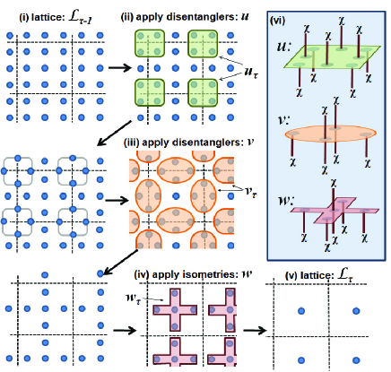
2D MERA.— Let us consider a square lattice made of sites, each one described by a Hilbert space of finite dimension . The proposed 2D MERA is characterized by the coarse-graining transformation of Fig. (1), where blocks of sites of lattice are mapped onto single sites of a coarser lattice . This is achieved in three steps: first disentanglers are applied on the four sites located at the corners of four adjacent blocks; then disentanglers are applied at the boundary between two adjacent blocks, transforming four sites into two; finally, isometries are used to map a block into a single effective site. In this way, tensors and isometric ,
| (1) |
transform the state of the lattice in which we are interested (typically the ground state of a local Hamiltonian ) into a state of the effective lattice through the sequence
| (2) |
To understand the role of these tensors, it is useful to think of the state as possessing three different kinds of entanglement: short-range entanglement residing at the corners of four adjacent blocks, short-range entanglement residing near the boundary shared by two blocks, and long-range entanglement. Then the disentanglers and are used to reduce the amount of short-range entanglement residing near the corners and boundaries of the blocks. In other words, in states and increasing amounts of short-range entanglement from have been removed. This fact facilitates significantly the job of the isometry , namely to compress into an effective site of those degrees of freedom in a block that still remain entangled (now mostly through long-range entanglement) with degrees of freedom outside the block. Thus, the resulting state still contains the long-range entanglement of , but most of its short-range entanglement is gone. We complete the above construction by noticing that a -dimensional space is often too small to accommodate all the relevant degrees of freedom left on a block. Accordingly, we shall describe the effective sites of with a space of larger dimension . This dimension determines both the accuracy and cost of the simulations.
The transformation of Fig. 1 can now be applied to lattice , producing a coarser lattice . More generally, if is finite, iterations will produce a sequence of lattices where the top lattice contains only a small number of sites and can be addressed with exact numerical techniques. Thus, given a Hamiltonian on , we can use the above RG transformation to obtain a sequence of Hamiltonians , then diagonalize to find its ground state , and finally recover the ground state of by reversing all the RG transformations:
| (3) |
This is precisely how the MERA is defined. Specifically, the MERA for is a tensor network containing (i) a top tensor, that describes , and (ii) layers of tensors (disentanglers and isometries), where each layer is used to invert one step of the coarse-graining transformation of Fig. 1 according to the sequence (3).
The technical details on how to numerically optimize the disentanglers and isometries of the MERA to approximate the ground state of are analogous to those discussed in Ref. NewAlgorithm for a 1D lattice and will not be repeated here. Instead, we focus on the key aspect that makes the present 2D scheme much more efficient than that of Refs. FreeFermions ; FreeBosons ; Finite2D . For this purpose, we consider an operator whose support is contained within a block of sites of lattice . Direct inspection shows that, no matter where this block is placed with respect to the disentanglers and isometries of Fig. 1, the support of the resulting coarse-grained operator is also contained within a block of sites of , and the same holds for any subsequent coarse-graining. This is in sharp contrast with the 2D scheme of Refs. FreeFermions ; FreeBosons ; Finite2D , where the minimal stable support of local observables (or ’width’ of past causal cones) corresponded to blocks of sites. In the present case, much smaller objects (operators acting on sites instead of sites) are manipulated during the calculations, resulting in the announced dramatic drop in simulation costs.
Benchmark calculations.— We have tested the proposed scheme by investigating low energy properties of the quantum Ising model with transverse magnetic field,
| (4) |
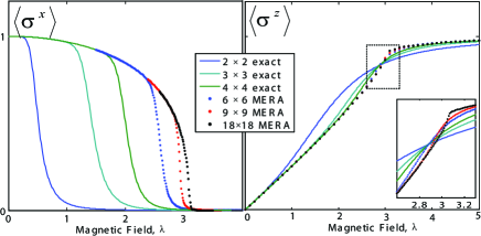
on a square lattice with periodic boundary conditions (local dimension ). First of all, we consider a sequence of lattices with increasing linear size . For each of them, a MERA approximation to the ground state of for different values of the transverse magnetic field is obtained using . Computing the ground state for and critical transverse magnetic field takes 4 days on a 3GHz dual-core desktop PC with 8Gb RAM when starting from a randomly initialized MERA chireduction . Fig. 2 displays the expected value of the parallel and transverse magnetizations, both of which show characteristic signs of a second order phase transition as increases. We emphasize that since the simulation costs grow only as the logarithm of , it is straightforward to increase the system size until e.g. finite size effects become negligible on local observables.
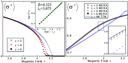
Fig. 3 shows how the parallel and transverse magnetizations change with increasing , for . Since the cost of the simulations grows as , only small values of can be considered in practice. However, with one already obtains estimates for the location of the critical point and the critical exponent that already fall within of the best Monte Carlo results MC .
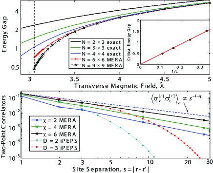
By using the MERA to represent a two-dimensional subspace and minimizing the expectation value of , we obtain the system’s energy gap . Fig. 4 shows as a function of the transverse magnetic field and system size. Notice that at the critical point the gap closes with the system size as (dynamic exponent ). Two-point correlators can also be extracted. Fig. 4 shows the correlator along a row or column of the lattice, obtained using the scale invariant algorithm CFT , which directly addresses an infinite lattice at the critical point.
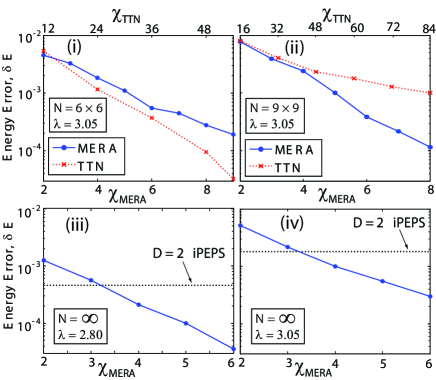
Role of disentanglers.— In order to highlight the importance of disentanglers, we have also performed simulations with a tree tensor network (TTN). This corresponds to a more orthodox real-space RG approach where the block of sites in Fig. 1 is directly mapped into an effective site without the use of disentanglers. Recall that a 2D ground state typically displays a boundary law, , for the entanglement entropy of a block of sites. To reproduce this boundary law with a TTN, one needs to increase the dimension at each step of the coarse-graining. Specifically, must grow doubly exponentially with the linear size of the lattice. On the other hand, the cost of manipulating a 2D TTN grows only as a small power of . As a result, much larger values of can be used with a TTN, leading to a very competitive approach for small lattice sizes TTN . Fig 5 (i and ii) compares the performance of the MERA and the TTN in lattices of size and . It shows that a TTN is more efficient than the MERA in computing the ground state of the lattice; however, this trend is already reversed in the lattice, where the cumulative benefit of using disentanglers clearly outweighs the large cost they incur. Disentanglers, by acting on the boundary of a block, readily reproduce the entropic boundary law (for any value of ) and allow us to consider arbitrarily large systems. Fig. 5 (iii and iv) shows results for an infinite lattice near and at criticality.
To summarize, we have proposed an entanglement renormalization scheme for the square lattice and demonstrated its scalability by addressing the quantum Ising model on systems of linear size , with cost , and on an infinite system at criticality, with cost . The key of the present approach is the use of two types of disentanglers that remove short-range entanglement residing near the corners and near the boundaries of the blocks while leading to narrow causal cones of sites. Similar schemes can be built e.g. for triangular, hexagonal and Kagome lattices kagMERA .
The authors thank Roman Orus, Luca Tagliacozzo and Philippe Corboz for comments. Support from the Australian Research Council (APA, FF0668731, DP0878830) is acknowledged.
References
- (1) G. Vidal, Phys. Rev. Lett. 99, 220405 (2007).
- (2) K.G. Wilson, Rev. Mod. Phys. 47, 773 (1975).
- (3) S. R. White, Phys. Rev. Lett. 69, 2863 (1992), Phys. Rev. B 48, 10345 (1993).
- (4) G. Vidal, Phys. Rev. Lett. 101, 110501 (2008).
- (5) G. Evenbly, G.Vidal, Phys. Rev. B 79, 144108 (2009).
- (6) M. Aguado, G. Vidal, Phys. Rev. Lett. 100, 070404 (2008). R. Koenig, B. Reichardt, G. Vidal, arXiv:0806.4583v1 [cond-mat.str-el].
- (7) G. Evenbly and G. Vidal, arXiv:0710.0692v2 [quant-ph].
- (8) G. Evenbly and G. Vidal, arXiv:0801.2449v1 [quant-ph].
- (9) V. Giovannetti, S. Montangero, R. Fazio, Phys. Rev. Lett. 101, 180503 (2008).
- (10) R. N. C. Pfeifer, G. Evenbly, G. Vidal, Phys. Rev. A. 79, 040301 (2009).
- (11) S. Montangero, M. Rizzi, V. Giovannetti, R. Fazio, arXiv:0810.1414v1 [quant-ph].
- (12) L. Cincio, J. Dziarmaga, M. M. Rams, Phys. Rev. Lett. 100, 240603 (2008)
- (13) L. Tagliacozzo, G. Evenbly, and G. Vidal, arXiv:0903.5017v1.
- (14) The tensors of the MERA are called disentanglers or isometries depending on whether they are in charge of eliminating short-range entanglement or of mapping a block of sites into a single site ER ; MERA ; NewAlgorithm . This distinction is somewhat arbitrary: one can consider tensors that fulfill the two roles simultaneously, such as tensor in Fig. 1, that we still call disentangler. All these tensors must be isometric, that is , , . The hermitian conjugation () in Eq. (1) appears for consistency with previous references.
- (15) Calculations for are achieved by using a disentangler with on selected indices. The computation time is reduced to a few hours per point by re-using a MERA previously converged (for a similar magnetic field) as the starting point of a simulation.
- (16) H. Rieger, N. Kawashima, Europ. Phys. J. B 9, 233 (1999). H.W.J. Blote and Y. Deng, Phys. Rev. E 66, 066110(2002).
- (17) A. Pelissetto, E. Vicari, Phys. Rept. 368, 549 (2002).
- (18) J. Jordan et al., Phys. Rev. Lett. 101, 250602 (2008)
- (19) G. Evenbly, G. Vidal, arXiv:0904.3383v1.