THE OPTX PROJECT I: THE FLUX AND REDSHIFT CATALOGS FOR THE
CLANS, CLASXS, AND CDF-N FIELDS

Abstract

We present the redshift catalogs for the X-ray sources detected in the Chandra Deep Field North (CDF-N), the Chandra Large Area Synoptic X-ray Survey (CLASXS), and the Chandra Lockman Area North Survey (CLANS). The catalogs for the CDF-N and CLASXS fields include redshifts from previous work, while the redshifts for the CLANS field are all new. For fluxes above $10^{-14}$ ergs cm^-2 s^-1 ($2-8~{}\rm keV$) we have redshifts for $76$% of the sources. We extend the redshift information for the full sample using photometric redshifts. The goal of the OPTX Project is to use these three surveys, which are among the most spectroscopically complete surveys to date, to analyze the effect of spectral type on the shape and evolution of the X-ray luminosity functions and to compare the optical spectral types with the X-ray spectral properties.

We also present the CLANS X-ray catalog. The nine ACIS-I fields cover a solid angle of $\sim$0.6 deg² and reach fluxes of $7\times 10^{-16}$ ergs cm^-2 s^-1 ($0.5-2~{}{\rm keV}$) and $3.5\times 10^{-15}$ ergs cm^-2 s^-1 ($2-8~{}{\rm keV}$). We find a total of 761 X-ray point sources. Additionally, we present the optical and infrared photometric catalog for the CLANS X-ray sources, as well as updated optical and infrared photometric catalogs for the X-ray sources in the CLASXS and CDF-N fields.

The CLANS and CLASXS surveys bridge the gap between the ultradeep pencil-beam surveys, such as the CDFs, and the shallower, very large-area surveys. As a result, they probe the X-ray sources that contribute the bulk of the $2-8~{}{\rm keV}$ X-ray background and cover the flux range of the observed break in the log$N-$log$S$ distribution. We construct differential number counts for each individual field and for the full sample.

1. INTRODUCTION

We combine data from the Chandra Deep Field North (CDF-N), the Chandra Large Area Synoptic X-ray Survey (CLASXS), and the Chandra Lockman Area North Survey (CLANS) to provide one of the most spectroscopically complete large samples of Chandra X-ray sources for use in the OPTX Project. In this article, the first in the OPTX Project series, we present the database that we use in Yencho et al. (2008) to examine the X-ray luminosity functions and their dependence on spectral classification and in L. Trouille et al. (2008, in preparation) to compare the optical spectral classifications with the X-ray spectral properties.

As a community, we have obtained a myriad of X-ray surveys, from deep pencil-beam to shallow wide-field surveys (see Figure 1 in Brandt & Hasinger 2005). The ultradeep surveys (CDF-N, Brandt et al. 2001 and Alexander et al. 2003; Chandra Deep Field South or CDF-S, Giacconi et al. 2002) have resolved nearly $100$% of the $2-8~{}\rm keV$ X-ray background (hereafter XRB; see Churazov et al. 2007 for a recent measurement of the XRB using INTEGRAL and Gilli et al. 2007 and Frontera et al. 2007 for in-depth comparisons of the various XRB measurements to date). The shallow (ASCA, Ueda et al. 1999; XBoötes, Murray et al. 2005) and intermediate-depth (SEXSI, Harrison et al. 2003; CLASXS, Yang et al. 2004; AEGIS, Nandra et al. 2005, Davis et al. 2007; extended-CDF-S, Lehmer et al. 2005, Virani et al. 2006a; XMM-COSMOS, Cappelluti et al. 2007; ChaMP, Kim et al. 2007a; and CLANS, this article) wide-area surveys improve statistics on active galactic nuclei (AGN) evolution and luminosity functions, detect the rarer sources (obscured QSOs and high-redshift AGNs), and uncover the extent of large-scale structure.

However, it is essential that these surveys be followed up spectroscopically as completely as possible. While deep multi-band photometry for surveys has made determining photometric redshifts possible (e.g., Rowan-Robinson et al. 2008 and references therein) and the reliability can be improved by incorporating near-infrared (NIR) and mid-infrared (MIR) data (Wang et al. 2006), with optical spectra of the X-ray sources we can both make redshift identifications and spectrally classify the sources. Throughout this paper, “identification” of redshifts is defined as the robust determination of a redshift from the observed optical spectrum. We can also use the optical spectra to compare optical emission line luminosities with X-ray luminosities (Mulchaey et al. 1994; Alonso-Herrero et al. 1997).

While other X-ray surveys have numerous redshifts, they are relatively incomplete in heterogeneous ways (see Table 1). In contrast, the present article is one in a series focusing on three of the most uniformly observed and spectroscopically complete surveys to date. The deep pencil-beam CDF-N survey is the most spectroscopically complete of all of the X-ray survey fields. Our group (Barger et al. 2002, 2003, 2005; present work) has spectroscopically observed 459 of the 503 X-ray sources in this field and has obtained reliable redshift identifications for 312. In comparison, of the 349 X-ray sources in the 1 Ms CDF-S, 251 have been spectroscopically observed and 168 have redshift identifications (Szokoly et al. 2004).

Our two intermediate-depth wide-area surveys provide an essential step between the ultradeep narrow Chandra surveys and the shallow wide-area surveys. They cover large cosmological volumes, detect rare, high-luminosity AGNs, and robustly probe AGN evolution between $z\sim 0$ and 1.

Yang et al. (2004) undertook an $\sim$0.4 deg² contiguous Chandra survey of the Lockman Hole-Northwest field. The Chandra Large Area Synoptic X-ray Survey (CLASXS) was designed to sample a large, contiguous solid angle, while remaining sensitive enough to measure $2-3$ times fainter than the observed break in the $2-8~{}\rm{keV}$ log$N-$log$S$ distribution. Our group (Steffen et al. 2004; present work) has spectroscopically observed 468 of the 525 X-ray sources in the CLASXS field and obtained reliable redshift identifications for 280.

In 2004 the Chandra/SWIRE team (PI, B. Wilkes) observed a solid angle of $\sim$0.6 deg² in a second field in the Lockman Area to a $2-8~{}\rm keV$ limiting flux of $3.5\times 10^{-15}$ ergs cm^-2 s^-1. This field is also part of the Spitzer Wide-Area Infrared Extragalactic Survey (SWIRE; Lonsdale et al. 2003, 2004), which surveyed approximately 65 deg² distributed over 7 fields in the northern and southern sky. Polletta et al. (2006) used Chandra/SWIRE to study the Spitzer selected sources in the field. Here we describe the Chandra survey in detail for the first time. For clarity, we have renamed it the Chandra Lockman Area North Survey (CLANS). We have spectroscopically observed 533 of the 761 X-ray sources in the CLANS field and have obtained reliable redshift identifications for 336.

In this paper we present the X-ray data for the CLANS field and the most up-to-date photometric and spectroscopic data of the optical and infrared counterparts to the X-ray sources for the CLANS, CLASXS, and CDF-N fields. In §2 we describe the CLANS X-ray observations and provide the X-ray catalog. We discuss our optical and infrared imaging data in §3, our redshift information in §4, and our optical spectral classifications in §5. In §6 we present the CLANS, CLASXS, and CDF-N optical and infrared photometric and spectroscopic catalogs. We calculate the rest-frame $2-8~{}\rm keV$ X-ray luminosities in §7, and in §8 we construct differential log$N-$log$S$ relations and compare our results with those of other surveys.

We use J2000 coordinates and assume $\Omega_{M}=0.3,\Omega_{\Lambda}=0.7$, and H${}_{0}=70$ km s^-1 Mpc^-1. All magnitudes are in the AB magnitude system and, unless otherwise specified, fluxes are in ergs cm^-2 s^-1.

2. X-RAY PROPERTIES

2.1. CLANS X-ray Observations

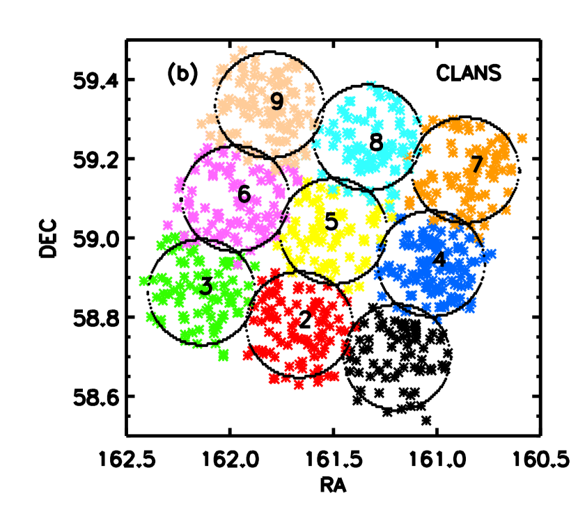
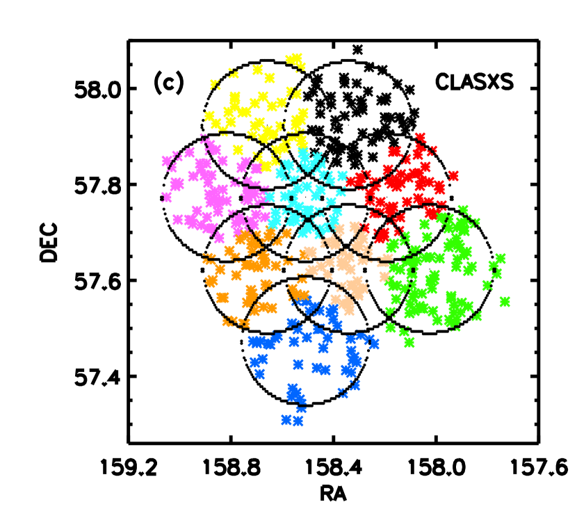
Figure 1.— (a) Location of the CLANS and CLASXS pointings in the Lockman Hole. The circles delimit $5\arcmin$ from the pointing centers (the area within which the sensitivity of source detection in the ACIS-I images is approximately uniform). Location of the (b) CLANS and (c) CLASXS X-ray sources. The circles delimit $8\arcmin$ from the pointing centers, which is the limiting off-axis angle used in §8 when calculating the log$N-$log$S$ distributions for these fields. The numbers 1-9 in (b) correspond to the Chandra/SWIRE Lockman pointings listed in Table 2.

To minimize the effects of Galactic attenuation, both the CLANS and CLASXS fields reside in the Lockman Hole high latitude region of extremely low Galactic HI column density ($5.7\times 10^{19}$ cm^-2; Lockman et al. 1986). The Galactic HI column density along the line of sight to the CDF-N is $1.6\times 10^{20}$ cm^-2 (Stark et al. 1992).

CLANS consists of nine separate $\sim$70 ks Chandra ACIS-I exposures centered at $(\alpha,\delta)_{J2000}=(10^{h}46^{m},+59^{\circ}01\arcmin$) (see Table 2) combined to create an $\sim$0.6 deg² image containing 761 sources. The X-ray flux limits are $f_{2-8~{}{\rm keV}}\sim 3.5\times 10^{-15}$ ergs cm^-2 s^-1 and $f_{0.5-2~{}{\rm keV}}\sim 7\times 10^{-16}$ ergs cm^-2 s^-1.

While the ACIS-I field of view is $17\arcmin\times 17\arcmin$, the sensitivity of the source detection is approximately uniform only within off-axis angles less than $\sim 5\arcmin$. As the off-axis angle increases, the sensitivity drops due to vignetting effects, quantum efficiency changes across the field, and the broadening of the point-spread functions (see Figure 3 and §2.5). Therefore, while the CLANS ACIS-I pointings exposed an almost contiguous area, the actual coverage, as evidenced by the gaps between the $5\arcmin$ circles in Figure 1a, is non-uniform. The survey was optimized to obtain the largest solid angle possible. The CLASXS survey, on the other hand, was designed to achieve uniform field coverage (at off-axis angles $\approx 5\arcmin$, the CLASXS pointings overlap slightly as shown in Figure 1a).

In Figures 1b and 1c we show $8\arcmin$ circles around the CLANS and CLASXS pointings. This is the limiting off-axis angle used in §8 when calculating the log$N-$log$S$ distributions for these fields. While there is substantial overlap between the CLASXS pointings at these off-axis angles, the CLANS pointings overlap very little. This is important in the determination of the effective areas for each field (see §2.5).

In Table 3 we list the characteristics of the CLANS field in terms of the Chandra exposure times, areas covered, X-ray flux limits, and total number of X-ray sources. We include the CLASXS and CDF-N characteristics for comparison.

2.2. CLANS X-ray Source Detection and Fluxes

Brandt et al. (2001) and Alexander et al. (2003) used the wavdetect tool included in the CIAO package (Freeman et al. 2002) to detect the X-ray sources in the CDF-N. Yang et al. (2004) also used wavdetect on the CLASXS field, in particular because the program uses a set of scales to optimize the source detection, making it excellent at separating nearby sources in crowded fields. In general, wavdetect provides better sensitivity than the classical sliding-box methods.

We ran wavdetect on the full-resolution CLANS images with wavelet scales of 1, $\sqrt{2}$, 2, 2$\sqrt{2}$, 4, 4$\sqrt{2}$, and 8. We used a significance threshold of $10^{-7}$, which translates to a probability of a false detection of 0.4 per ACIS-I field based on Monte Carlo simulation results (Freeman et al. 2002).

We used the aperture photometry tool for source flux extraction described in detail in Yang et al. (2004). The method uses circular extraction cells. We linearly interpolated the CIAO Library PSFs to the off-axis angles and $\sim 95$% of the enclosed energies for each source. In the $0.5-2~{}\rm keV$ ($2-8~{}\rm keV$) band, the 95% encircled radius is equal to $2.5\arcsec$ at an off-axis angle of $3\arcmin$ ($2\arcmin$) and is equal to $9.5\arcsec$ ($10\arcsec$) at an off-axis angle of $8\arcmin$. For a plot of the variation of the 95% encircled radius with off-axis angle, see Figure 3 in Yang et al. (2004). If the determined PSF value were greater than 2$\farcs$5, then we used it as the radius of the circular extraction cell for that source and applied an aperture correction to the final flux determination. If it were less than 2$\farcs$5, then we used a fixed 2$\farcs$5 radius. As described in Yang et al. (2004), we estimated the background using an eight-piece segmented annulus region four times as large as the source cell area, with an inner radius $5\arcsec$ larger than the source cell radius. We excluded any segments containing more counts than the 3$\sigma$ Poisson upper limit in order to avoid nearby sources. We then determined the background surface brightness by dividing the counts by the area enclosed in the remaining segments. By multiplying this background surface brightness by the area within the circular extraction cell, we determined the background counts. We obtained the net counts by subtracting the background counts from the counts within the circular extraction cell.

We then made full-resolution spectrally weighted exposure maps. We used these exposure maps only to correct for vignetting. We computed the flux conversion at the aim point using spectral modeling (using monochromatic maps does not change the results significantly). For each source we convolved the exposure map with the PSF generated using mkpsf and normalized it to the exposure time at the aim point. This gives the effective exposure time if the source is at the aim point. In XSPEC we obtained the count rate to flux conversion factor at the aim point by assuming each source has a single power law spectrum with Galactic absorption (using the CIAO-scripts mkacisrmf and mkarf to generate the necessary RMF and ARF files). We calculated the power law photon index, $\Gamma$, for each source using the hardness ratio, defined as HR$\equiv$C${}_{2-8~{}\rm keV}$/C${}_{0.5-2~{}\rm keV}$, where C${}_{2-8~{}\rm keV}$ and C${}_{0.5-2~{}\rm keV}$ are the count rates. For a more detailed description and analysis of this flux conversion method, see Yang et al. (2004).

Table 1Spectroscopic Completeness of Selected Surveys from the Literature

	eCDF-S	AEGIS	SEXSI	ChaMP
Area (deg2)	0.3	0.5	2	9.6
X-ray Flux Limit (10-16 ergs cm2 s-1)	6.7	8.2	300	9.0
Optical Limit for Spectroscopic Follow-up	$R_{AB}<25$	$R_{AB}<24.1$	$R_{AB}<24$	$r_{AB}^{\prime}<24$
Spectroscopic Completeness	35%	$\cdots$	40-70%	54%

Table 2CLANS Observation Summary

					Exposure
Target Name	Observation ID	$\alpha_{2000}$	$\delta_{2000}$	Observation Start Date	(ks)
SWIRE LOCKMAN 5 (center)	5023	10 46 00.00	+59 01 00.00	2004 Sept 12 21:30:56	67
SWIRE LOCKMAN 1	5024	10 44 46.15	+58 41 55.45	2004 Sept 16 06:53:47	65
SWIRE LOCKMAN 2	5025	10 46 39.44	+58 46 51.24	2004 Sept 17 20:30:04	70
SWIRE LOCKMAN 3	5026	10 48 32.77	+58 51 47.33	2004 Sept 18 16:17:12	69
SWIRE LOCKMAN 4	5027	10 44 06.67	+58 56 05.28	2004 Sept 20 14:40:35	67
SWIRE LOCKMAN 6	5028	10 47 53.44	+59 05 57.00	2004 Sept 23 03:36:12	71
SWIRE LOCKMAN 7	5029	10 43 27.23	+59 10 15.07	2004 Sept 24 03:43:15	71
SWIRE LOCKMAN 8	5030	10 45 20.56	+59 15 11.16	2004 Sept 25 19:47:08	66
SWIRE LOCKMAN 9	5031	10 47 13.85	+59 20 06.95	2004 Sept 26 14:47:00	65

Table 3X-ray Data Specifications

Category	CLANS	CLASXS	CDF-N
Exposure Time	$\sim 70$ ks	$\sim 40$ ks (73 ks)	2 Ms
Area (deg2)	0.6	0.45	0.124
$0.5-2~{}\rm keV$ Flux Limit	$7$	$12$ ($7$)	$0.25$
$2-8~{}\rm keV$ Flux Limit	$35$	$60$ ($35$)	$1.5$
Total # of X-ray Sources	761	525	503

Table 4CLANS X-ray Catalog: Basic Source Properties

		$\Delta\alpha$	$\Delta\delta$
Num.	$\alpha_{2000}$	$\delta_{2000}$	(arcsec)	(arcsec)	$f_{0.5-2~{}{\rm keV}}$	$f_{2-8~{}{\rm keV}}$	$f_{0.5-8~{}{\rm keV}}$	HR	$\Gamma$
(1)	(2)	(3)	(4)	(5)	(6)	(7)	(8)	(9)	(10)
1	160.58846	59.25157	0.831	0.457	3.37${}_{-0.51}^{+0.70}$	11.82${}_{-2.31}^{+2.80}$	14.36${}_{-1.80}^{+2.17}$	0.79${}_{-0.20}^{+0.25}$	1.05${}_{-0.26}^{+0.25}$
2	160.64172	59.17641	0.301	0.239	7.79${}_{-0.83}^{+0.97}$	10.01${}_{-1.75}^{+2.28}$	17.98${}_{-1.62}^{+1.94}$	0.37${}_{-0.08}^{+0.10}$	1.71${}_{-0.19}^{+0.20}$
3	160.64175	59.16873	0.710	0.376	0.63${}_{-0.22}^{+0.38}$	0.75${}_{-0.52}^{+0.79}$	1.45${}_{-0.50}^{+0.60}$	0.34${}_{-0.27}^{+0.42}$	1.76${}_{-0.69}^{+0.78}$
4	160.65615	59.11504	1.231	0.581	1.52${}_{-0.57}^{+1.01}$	0.51${}_{-0.42}^{+1.74}$	2.20${}_{-0.67}^{+1.30}$	0.13${}_{-0.12}^{+0.46}$	2.37${}_{-1.08}^{+0.36}$
5	160.66704	59.07057	0.983	0.559	1.19${}_{-0.31}^{+0.46}$	6.34${}_{-1.83}^{+2.12}$	7.88${}_{-1.51}^{+1.83}$	1.09${}_{-0.42}^{+0.56}$	0.74${}_{-0.13}^{+0.44}$
6	160.66924	59.25401	1.004	0.460	0.93${}_{-0.28}^{+0.37}$	4.63${}_{-1.38}^{+1.86}$	5.86${}_{-1.21}^{+1.49}$	1.03${}_{-0.44}^{+0.59}$	0.80${}_{-0.18}^{+0.49}$
..	..	..	..	..	..	..	..	..	..

Table 5CLANS X-ray Catalog: Additional Source Properties

				t${}_{0.5-2~{}\rm keV}$	t${}_{2-8~{}\rm keV}$	t${}_{0.5-8~{}\rm keV}$	R
Num.	n${}_{0.5-2~{}\rm keV}$	n${}_{2-8~{}\rm keV}$	n${}_{0.5-8~{}\rm keV}$	($10^{4}$ s)	($10^{4}$ s)	($10^{4}$ s)	(arcminutes)
(1)	(2)	(3)	(4)	(5)	(6)	(7)	(8)
1	36.50${}_{-5.56}^{+7.63}$	26.00${}_{-5.07}^{+6.16}$	59.75${}_{-7.48}^{+9.04}$	5.90	5.34	5.80	9.7
2	83.75${}_{-8.90}^{+10.45}$	29.75${}_{-5.20}^{+6.78}$	112.50${}_{-10.12}^{+12.16}$	6.47	6.26	6.40	6.8
3	6.75${}_{-2.35}^{+4.01}$	2.25${}_{-1.57}^{+2.38}$	9.25${}_{-3.21}^{+3.85}$	6.48	6.28	6.41	6.8
4	5.75${}_{-2.15}^{+3.83}$	0.75${}_{-0.62}^{+2.54}$	7.50${}_{-2.28}^{+4.44}$	2.71	2.62	2.65	7.2
5	12.75${}_{-3.32}^{+4.94}$	13.25${}_{-3.82}^{+4.44}$	27.00${}_{-5.17}^{+6.26}$	5.65	5.40	5.54	8.5
6	11.00${}_{-3.28}^{+4.41}$	11.00${}_{-3.28}^{+4.41}$	23.00${}_{-4.77}^{+5.86}$	6.27	6.07	6.20	7.8
..	..	..	..	..	..	..	..

2.3. CLANS X-ray Catalog

The CLANS observations consist of a 3$\times$3 raster with an $\sim 2\arcmin$ overlap between continguous pointings (Polletta et al. 2006; see our Figure 1). Following the prescription in Yang et al. (2004) for the CLASXS field, we merged the nine individual pointing catalogs to create the final CLANS X-ray catalog. For sources with more than one detection in the nine fields, we used the detection from the observation in which the effective area of the source was the largest.

We present the CLANS X-ray catalog in Tables 4 and 5. In both tables, column (1) is the source number. The numbers correspond to ascending order in right ascension. In Table 4, columns (2) and (3) give the right ascension and declination coordinates of the X-ray sources. Columns (4) and (5) list the 95% confidence errors from wavdetect on these right ascension and declination coordinates. Columns (6), (7), and (8) provide the X-ray fluxes in the $0.5-2~{}\rm keV$, $2-8~{}\rm keV$, and $0.5-8~{}\rm keV$ bands, respectively, in units of 10^-15 ergs cm^-2 s^-1. The errors quoted are the $1\sigma$ Poisson errors, using the approximations from Gehrels (1986). They do not include the uncertainty in the flux conversion factor; however, the errors are generally dominated by the Poisson errors. Column (9) gives the hardness ratio, as defined in §2.2. Column (10) lists the value of $\Gamma$ for each source. The errors in Columns 9 and 10 are the $1\sigma$ errors propagated from the $1\sigma$ errors on the counts listed in Table 5.

In Table 5, columns (2), (3), and (4) list the net counts in the $0.5-2~{}\rm keV$, $2-8~{}\rm keV$, and $0.5-8~{}\rm keV$ bands, respectively. The errors quoted are the $1\sigma$ Poisson errors, using the approximations from Gehrels (1986). Columns (5), (6), and (7) give the effective exposure times from the exposure maps in each of the three energy bands. Column (8) provides the distance from the pointing center for each source.

2.4. Flux Limits

Following the prescription in Alexander et al. (2003), we determined the flux limits for a signal-to-noise ratio ($S/N$) of 3 for the CLANS and CLASXS fields. To determine the sensitivity across the field it is necessary to take into account the broadening of the PSF with off-axis angle, as well as changes in the effective exposure and background rates across the field. Under the simplifying assumption of $\sqrt{N}$ uncertainties, we can determine the sensitivity across the field following Muno et al. (2003) as

$$S=\frac{n_{\sigma}^{2}}{2}(1+[1+\frac{8b}{n_{\sigma}^{2}}]^{1/2}),$$ (1)

where $S$ is the number of source counts and $b$ is the number of background counts in a source cell. The $n_{\sigma}$ is the required signal-to-noise ratio.

After setting $n_{\sigma}=3$, the only component within Equation 1 that we need to measure is the background counts. We determined the median number of background counts at each off-axis angle (using the method described in §2.2) and inputted this into Equation 1 to determine $S$ at each off-axis angle. Using the flux conversion method discussed in §2.2, we converted $S$ from counts to flux values.

The red lines in Figure 2 show the flux limits (for a $S/N=3$) versus the off-axis angle. The green circles (black squares) identify the sources whose fluxes are greater (less) than the corresponding flux limit. Because all of the CLANS pointings have exposure times of $\sim$70 ks, there is only a single red line that increases slightly in flux as the off-axis angle increases. In the CLASXS field, however, the LHNW-1 pointing has an exposure time of 73 ks, while the other pointings are all $\sim$40 ks. Thus, the dashed red line located at slightly lower fluxes than the solid red line shows the flux limits corresponding to the deeper 73 ks ACIS-I pointing. The bottom plots in Figure 2 show the Alexander et al. (2003) flux limits (for a $S/N=3$) for the CDF-N field.

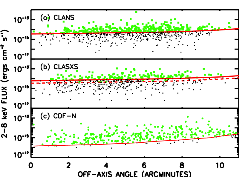
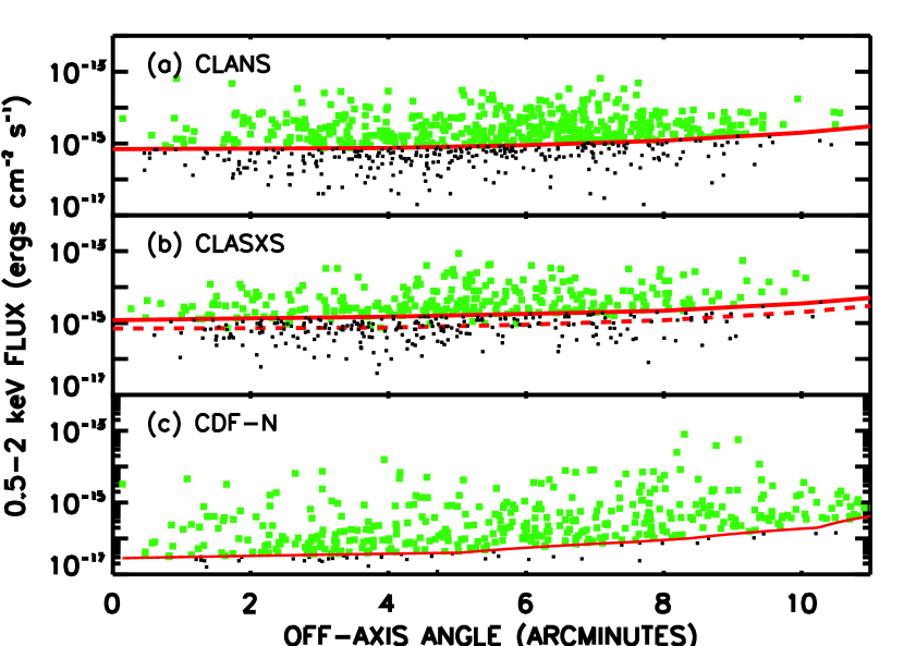
Figure 2.— $2-8~{}\rm keV$ and $0.5-2~{}\rm keV$ flux versus off-axis angle for the X-ray sources in the CLANS, CLASXS, and CDF-N fields (red lines, $S/N=3$ flux limits at the off-axis angle of each source detected by wavdetect; dashed red lines, $S/N=3$ flux limits for the deeper $73~{}$ks pointing in the CLASXS field; green circles, sources with fluxes greater than the corresponding flux limit; black squares, sources with fluxes below the corresponding flux limit).

2.5. Effective Areas

Yang et al. (2004, 2006) used Monte Carlo simulations of the CLASXS 40 ks and 70 ks $2-8~{}\rm keV$ and $0.5-2~{}\rm keV$ band ACIS-I images to examine the incompleteness in their number counts. The sensitivity of the source detection drops with off-axis angle due to vignetting effects, quantum efficiency changes across the field, and the broadening of the point-spread functions. Using wavdetect on their simulated images, Yang et al. obtained an estimate of the detection probability function, or probability that a source would be detected by wavdetect, at different fluxes and off-axis angles.

The differences at small and large off-axis angles between their 2004 and 2006 simulations are attributable to two methodological changes. First, in their 2004 simulations they used many fewer simulated sources, causing an undersampling at small off-axis angles. Second, in their 2004 simulations they did not use large wave scales, causing a quick drop in source detection at off-axis angles greater than $6\arcmin$.

We interpolated from their 40 ks and 70 ks 2006 simulations to the exposure times for the nine pointings in both the CLANS and CLASXS fields, respectively (see Table 2 for the CLANS field exposure times and Yang et al. 2004 Table 1 for the CLASXS field exposure times) to determine the probability of detection for a source at a given off-axis angle and flux in each pointing. Figure 3 shows the probability of source detection as a function of off-axis angle and $2-8~{}\rm{keV}$ flux for the central CLANS pointing (Chandra/SWIRE Lockman 5 in Table 2) with an exposure time of 67 ks. As expected, the probability of detecting a source at a given off-axis angle decreases as the flux of the source decreases.

We then determined the effective sky area for each pointing using the formula

$$A(f_{x})=\int_{0}^{a}2\pi a~{}da~{}D(a,f_{x})~{}g(a),$$ (2)

where $a$ is the off-axis angle from the pointing center, $g(a)$ is the geometric fraction, and $D(a,f_{x})$ is the detection probability, equivalent to an incompleteness factor.

Figure 4 shows the geometric fraction, or fraction of the total area covered by an annulus of width $0\farcm 5$ and outer radius $a$ that is contained within the ACIS-I chip. Figure 4a shows our ULBCam $H$-band image (see §3.3) of the CLANS field overlaid with the ACIS-I chip outline (the square) and two annuli with off-axis angles $7\arcmin-7\farcm 5$ and $9\farcm 5-10\arcmin$. Figure 4(b) shows that the geometric fraction is 1 for all annuli with outer radii less than $\sim 8\arcmin$. At $a>8\arcmin$, $g(a)$ decreases rapidly.

We determined $A(f_{x})$ for 5 different limiting detection probabilities, 20%, 30%, 50%, 70%, and 90%. In the determination of $A(f_{x})$, if the simulated $D(a,f_{x})$ at the off-axis angle of a source of flux $f_{x}$ were found to be below this limiting detection probability, then we assigned $D(a,f_{x})=0$ for that source.

Because the sensitivity of Chandra degrades at large off-axis angles, we exclude sources with off-axis angles greater than $8\arcmin$ in our number counts determination (see §8). In the CLANS field at these off-axis angles there is little overlap between pointings, so $\Omega(f_{x})\approx\sum A_{i}(f_{x})$. However, in the CLASXS field the pointings overlap significantly (as shown in Figure 1). We used the ds9 funtools function that determines area within region files to subtract the overlapping area from the total $\Omega(f_{x})$ value. We also made sure that any area that had already been subtracted as part of the geometric fraction determination was not subtracted a second time at this stage.

Figure 5 shows the total true effective area, $\Omega$, versus flux for (a) the 20%, 30%, 50%, 70%, and 90% probability of detection cases for the CLANS field and (b) the 30% probability of detection case for the CLASXS field. The dashed line shows the effective area if $D(a,f_{x})=1$ is set for all fluxes and off-axis angles, in other words, where $\Omega=9\times\int_{0}^{a}2\pi a~{}da~{}g(a)$ minus any overlapping areas between pointings.

This figure shows that the small off-axis angles (or small $\Omega$ values) probe the faintest fluxes, since the Chandra sensitivity is highest close to the pointing center. Figure 5a also shows that we can probe to fainter fluxes at the expense of more incompleteness, since the lower we push our probability of detection, the fainter the flux probed at a given off-axis angle.

In our calculation of the log$N-$log$S$ distribution (see §8), we use the results from the 30% probability of detection case. Although this is a fairly arbitrary choice, we chose it to maximize depth while not using too low of a probability of detection.

Figure 3.— Probability of source detection as a function of off-axis angle and $2-8~{}\rm{keV}$ flux for the 67 ks central CLANS pointing. To obtain these results, we interpolated from the Yang et al. (2006) simulations for 40 ks and 70 ks exposure times.

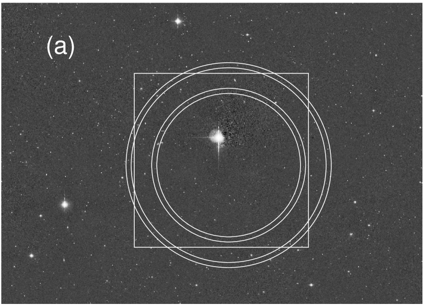
Figure 4.— (a) ACIS-I chip outline overlaid on the ULBCam $H$-band image of the CLANS field. Two annuli (off-axis angles $7\arcmin-7\farcm 5$ and $9\farcm 5-10\arcmin$) are shown in white. Note the offset of the chip center from the pointing center. (b) Fraction of the total area covered by an annulus of width $0\farcm 5$ that is contained within the ACIS-I chip versus the annulus’ outer radius.

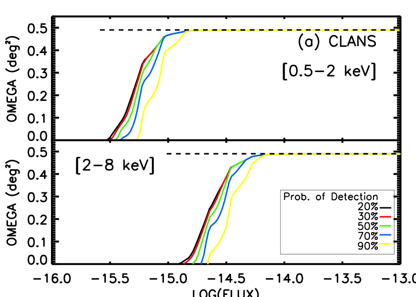
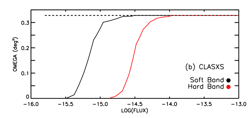
Figure 5.— Total true effective area, $\Omega$, versus $0.5-2~{}\rm keV$ and $2-8~{}\rm keV$ flux for off-axis angles $<8\arcmin$ for (a) the CLANS field (for the 20%, 30%, 50%, 70%, and 90% probability of detection cases) and (b) the CLASXS field (for only the 30% probability of detection case). The dashed line shows the effective area if $D(a,f_{x})=1$ is set for all fluxes and off-axis angles (i.e., where $\Omega=9\times\int_{0}^{a}2\pi a~{}da~{}g(a)$ minus any overlapping areas between pointings).

3. OPTICAL AND IR IMAGING

In this section we present new $g^{\prime},r^{\prime},i^{\prime},z^{\prime},J,H$, and $K$ photometry for the CLANS X-ray sources (see Table 6), new $u,g^{\prime},i^{\prime},J,H$, and $K$ photometry, as well as updated $B,V,R,I,$ and $z^{\prime}$ photometry, for the CLASXS X-ray sources (see Table 7 and §3.7), and new $J,H,$ and $K_{s}$ photometry for the CDF-N X-ray sources (see Table 8). We also present the Spitzer $3.6~{}\mu$m and $24~{}\mu$m data for all three fields (see §3.5).

3.1. MegaCam

The CFHT MegaCam/Megaprime camera has a 1 deg² field of view on the 3.6 m CFHT telescope. The focal plane is covered with 36 $2$k$\times 4.5$k EEV CCD detectors with excellent response between 3200 Å and 9000 Å (Aune et al. 2003; Boulade et al. 2003).

We used MegaCam to obtain deep $g^{\prime},r^{\prime},i^{\prime}$, and $z^{\prime}$-band data for the CLANS field and deep $u,g^{\prime}$, and $i^{\prime}$-band data for the CLASXS field. Observations were taken in sets of 7-point dithered exposures forming a circular pattern. The radius of the dither circle was $7\farcs 5$, which was enough to fill the chip gaps but minimized the chip overlap.

The CFHT operates in queue observing mode for MegaCam observations, which ensures uniform image quality and photometry, and a standard reduction pipeline (Elixir) is provided by CFHT and TERAPIX. The queue observer takes calibration frames each night, which the Elixir pipeline uses to calibrate the data (Magnier & Cuillandre 2004). The pipeline corrects for bias, dark current, flatfielding, and scattered light, with the final photometric calibration better than 1% across the field of view.

The TERAPIX data processing center provided further reduction of our data including astrometric and photometric calibration, sky subtraction, and image combination. At TERAPIX the ‘qualityFITS’ data quality assessment tool was used to visually inspect the calibrated images provided by Elixir and any defective images were rejected. Images with a seeing larger than $1\farcs 25$ in the $g^{\prime},r^{\prime},i^{\prime},$ and $z^{\prime}$-band and larger than $1\farcs 35$ in the $u$-band were also rejected.

3.2. WIRCam

We obtained our $K_{s}$-band photometry for the CDF-N using WIRCam on CFHT. We used our own IDL program to stack the images into a final mosaic, remove cosmic rays, establish a background estimation, align the astrometry to the USNO catalog, and derive a final zeropoint via comparison with 2MASS. More details of the observations and reductions can be found in Barger et al. (2008).

3.3. ULBCam

We carried out deep $J$- and $H$-band imaging of the three fields using the Ultra-Low Background Camera (ULBCam) on the University of Hawaii 2.2 m telescope during $2003-2006$. ULBCam consists of four 2k$\times$2k HAWAII-2RG arrays (Loose et al. 2003) with a total $16\arcmin\times 16\arcmin$ field of view. We took the images using a 13-point dither pattern with $\pm 30\arcsec$ and $\pm 60\arcsec$ dither steps in order to cover the chip gaps. We flattened the data using median sky flats from each dither pattern and corrected the image distortion using the astrometry in the USNO-B1.0 catalog (Monet et al. 2003). We combined the flattened, sky-subtracted, and warped images to form the final mosaic. A more extensive description of the data reduction and a detailed analysis is given in R. Keenan et al. (2008, in preparation).

3.4. WFCAM

We used WFCAM on the 3.8 m UKIRT telescope for our $K$-band photometry of the CLANS and CLASXS fields. The WFCAM camera has an 0.8 deg² field and is composed of four Rockwell Hawaii-II 2048$\times$2048 18 $\mu$m pixel array detectors, with a pixel scale of $0\farcs 4$. Acquired data are shipped from UKIRT to the Cambridge Astronomical Survey Unit (CASU). At CASU the WFCAM pipeline processes the data to produce stacked imaging data. The reduction steps are described in detail by Dye et al. (2006). Briefly, dark frames secured at the beginning of the night are subtracted from each target frame to remove bad pixels and amplifier glow and to reset anomalies from the raw frames. Twilight flats are then used to flatfield the data. The dithered frames are combined by weighted averaging (using a confidence map derived largely from the flatfield frames) to produce stacked frames.

The WFCAM Science Archive (WSA) archives all reduced WFCAM data. Each stacked frame contains four individual images, one for each of the four WFCAM cameras. After we retrieved the reduced data from WSA, we used our own IDL program to apply another background subtraction and astrometry check, to combine the four tiles into one frame, and to align the astrometry to the USNO catalog. A more extensive description of the data reduction is given in R. Keenan et al. (2008, in preparation).

3.5. Spitzer

To improve our photometric redshift determinations in the CLANS and CLASXS fields, we obtained $3.6~{}\mu$m data from the Spitzer Wide-Area Infrared Extragalactic Survey (SWIRE; Lonsdale et al. 2003) Legacy Science Program. We used the online NASA/IPAC Infrared Science Archive via GATOR to retrieve the $3.6~{}\mu$m and $24~{}\mu$m photometric catalogs, using a search radius of 2$\arcsec$ around our NIR counterpart source locations. The $3.6~{}\mu$m ($24~{}\mu$m) catalog has a $5\sigma$ limit of $5~{}\mu$Jy ($230~{}\mu$Jy) (Polletta et al. 2006).

Polletta et al. (2006) carried out an extensive analysis of the probability of false matches to the Spitzer IRAC catalogs for the CLANS field. Of the 774 X-ray sources in their catalog, they expect $\approx 19$ false assocations. We find a similar result of 23 false matches to the IRAC catalog using a simple randomization of our 761 CLANS X-ray sources. We find only 2 false matches to the MIPS catalog, which has many fewer sources than the IRAC catalog. The IRAC and MIPS data provide complete coverage for the CLANS field area. However, while the MIPS data provide complete coverage for the CLASXS field area, the IRAC data only cover 305 of the 525 CLASXS X-ray sources.

For the CDF-N X-ray sources, we obtained the relevant $3.6~{}\mu$m and $24~{}\mu$m data from the Great Observatories Origins Deep Survey-North (GOODS-N) Spitzer Legacy Science Project. We followed the method described in detail in Wang et al. (2006) to determine the $3.6~{}\mu$m Spitzer magnitudes from the GOODS-N first, interim, and second data release products (DR1, DR1+, DR2; M. Dickinson et al. 2008, in preparation). For the $24~{}\mu$m data, we used the DR1 + MIPS source list and the version 0.36 MIPS map provided by the Spitzer Legacy Program. The MIPS catalog is flux-limited and complete at $80~{}\mu$Jy and the median $1\sigma$ sensitivity of the MIPS map is $6.4~{}\mu$Jy. The $5\sigma$ sensitivity limit for the $3.6~{}\mu$m data is $0.327~{}\mu$Jy (Wang et al. 2006). Of the 503 CDF-N X-ray sources, 379 are in the area covered by the GOODS-N $3.6~{}\mu$m and $24~{}\mu$m micron observations.

Of the 761 CLANS, 305 CLASXS, and 379 CDF-N X-ray sources observed in the IRAC $3.6~{}\mu$m band, 633 CLANS, 249 CLASXS, and 351 CDF-N sources are detected to the limits of the SWIRE and GOODS-N surveys.

Of the 761 CLANS, 525 CLASXS, and 379 CDF-N X-ray sources observed in the MIPS $24~{}\mu$m band, 222 CLANS, 119 CLASXS, and 200 CDF-N sources are detected to the limits of the SWIRE and GOODS-N surveys.

Table 6CLANS Optical & Near-IR Specifications

Filter	Telescope	Average Seeing	$3\sigma$ Limit	Total Area
		(arcsec)	(AB mag)	(deg2)
$g^{\prime}$	CFHT	0.8	26.9	0.96
$r^{\prime}$	CFHT	1.1	26.5	1.16
$i^{\prime}$	CFHT	0.9	26.0	1.21
$z^{\prime}$	CFHT	0.9	25.3	1.33
$J$	UH 2.2 m	0.9	24.0	0.86
$H$	UH 2.2 m	0.9	23.2	0.83
$K$	UKIRT	1.2	22.1	0.74

Table 7CLASXS Optical & Near-IR Specifications

Filter	Telescope	Average Seeing	$3\sigma$ Limit	Total Area
		(arcsec)	(AB mag)	(deg2)
$u$	CFHT	1.3	25.9	1.16
$g^{\prime}$	CFHT	0.9	27.1	0.96
$i^{\prime}$	CFHT	1.0	25.3	1.12
$J$	UH 2.2 m	0.9	24.3	0.76
$H$	UH 2.2 m	1.1	23.1	0.68
$K$	UKIRT	1.0	22.1	0.74

Table 8CDF-N Near-IR Specifications

Filter	Telescope	Average Seeing	$3\sigma$ Limit	Total Area
		(arcsec)	(AB mag)	(deg2)
$J$	UH 2.2 m	1.2	24.7	0.25
$H$	UH 2.2 m	1.2	24.8	0.29
$K_{s}$	CFHT	0.8	24.2	0.29

3.6. Optical and NIR Source Detection and Photometry

We performed source detection and determined optical and NIR magnitudes using SExtractor (Bertin & Arnouts 1996). We set the detection threshold at eight contiguous pixels with counts at least 2$\sigma$ above the local sky background. Using the ASSOC_PARAMS function, we searched a $2\farcs 5$ radius around the X-ray point source location in the $z^{\prime}$-band image to determine the nearest optical counterpart location. We then used this $z^{\prime}$-band optical counterpart location to determine the magnitudes in the other bands. If there was no $z^{\prime}$-band optical counterpart but there was a $g^{\prime}$-band counterpart within the $2\farcs 5$ radius, we used this location instead. We then checked all sources by eye to ensure that the same source was being used to determine the optical and NIR magnitudes. In the CDF-N, for which we only present new NIR photometry, we used the Barger et al. (2003) X-ray source optical counterpart locations.

For sources with $z^{\prime}<21$, we used the MAG_AUTO magnitudes. For $z^{\prime}>21$, we used the $3\arcsec$ aperture-corrected magnitudes. We determined these by taking the ${3\arcsec}$ MAG_APER magnitude for each source and then applying an offset. We calculated the offset as the median difference between the $3\arcsec$ MAG_APER and $6\arcsec$ MAG_APER magnitudes for sources with $18<z^{\prime}<20$. The typical offset is 0.2 magnitudes with a $1\sigma$ error of 0.06. As expected, there is a slight trend towards smaller offsets with increasing magnitude ($\delta_{offset}<0.05$ magnitudes). Between $18<z^{\prime}<20$, the MAG_AUTO and $6\arcsec$ MAG_APER magnitudes generally agree well, with the MAG_AUTO magnitudes 0.01-0.03 magnitudes fainter than the $6\arcsec$ MAG_APER magnitudes. See R. Keenan et al. (2008, in preparation) for a more detailed discussion.

As stated above, in the catalogs we include magnitudes for sources with counts at least $2\sigma$ above the local sky background (as determined by SExtractor). We provide the aperture-corrected $3\sigma$ limits of the images in Tables 6, 7, and 8, which show the depth of our optical and NIR data. We determined these limits by laying down random $3\arcsec$ apertures away from objects on the images. We masked out the areas around bright stars to prevent erroneous detections and measurements from scattered light. We derived the aperture-corrected $3\sigma$ limit for each image from

$$3\sigma = -2.5\log(3~{}RMS\sqrt{\pi\times(1\farcs 5/platescale)^{2}})$$ (3)

$$+ZP~{}+OFFSET,$$

where RMS is the average standard deviation of the blank apertures, ZP is the zeropoint for the image in question, and OFFSET is the aperture-correction as discussed in the previous paragraph. A more detailed description of this method is given in R. Keenan et al. (2008, in preparation).

Typical $1\sigma$ errors on the CLANS $g^{\prime},r^{\prime},i^{\prime},z^{\prime},J,H,K,3.6~{}\mu$m and $24~{}\mu$m fluxes are 0.2, 0.3, 0.4, 0.9, 3.3, 7.2, 4.8, 10.2, and $629.9\times 10^{-30}$ ergs cm^-2 s^-1 Hz^-1, respectively. For the CLASXS field, typical $1\sigma$ errors for the $u,g^{\prime},i^{\prime},J,H,K,3.6~{}\mu$m and $24~{}\mu$m fluxes are 0.2, 0.2, 0.9, 2.4, 5.4, 3.6, 10.2, and $629.9\times 10^{-30}$ ergs cm^-2 s^-1 Hz^-1, respectively. And typical $1\sigma$ errors for the CDF-N $J,H,K,3.6~{}\mu$m and $24~{}\mu$m fluxes are 1.5, 1.3, 0.8, 0.5, and $64.0\times 10^{-30}$ ergs cm^-2 s^-1 Hz^-1, respectively.

3.7. CLASXS: Updated Optical Photometry

The original CLASXS catalog of Steffen et al. (2004) presented $B,V,R,I$, and $z^{\prime}$ photometry from CFHT and Subaru observations for 521 of the 525 X-ray point sources. When comparing the spectral energy distributions (SEDs) using these data with our more recent $u,g^{\prime}$, and $i^{\prime}$-band CFHT observations, we found that the original zeropoints for all but the $B$-band data were incorrect. The zeropointing errors reflect the difficulty of calibrating the Subaru Suprime-Cam images. Due to Subaru’s large collecting area, calibration stars saturate even with the shortest possible exposure times. Also, the Steffen et al. (2004) CFHT data were taken using CFH12K, which does not operate in queue mode, so no automatic calibrations were done (in contrast with the standard MegaCam queue mode procedure).

To determine the zeropoint offsets, we compared SEDs created from the Steffen et al. (2004) CFH12K data with SEDs made from the more recently obtained $u,g^{\prime}$, and $i^{\prime}$-band MegaCam data. We restricted our sample to sources with $21<g^{\prime}<23$. The zeropoint offsets listed in Table 9 are the mean of the values needed to shift the SEDs made from the original CFHT data onto the SEDs made from the new $u,g^{\prime}$, and $i^{\prime}$-band data.

We did this separately for the SEDs with a more obvious bluer slope (ascending SED as frequency increases) and those with a more obvious redder slope (descending SED as frequency increases), and found no major differences in the offsets between these two types of sources. We found that the CFHT $B$-band data had a negligible offset while the $R$- and $z^{\prime}$-band data were best re-zeropointed using an offset of -0.6.

We followed the same method to re-zeropoint the original Subaru $V,R,I$, and $z^{\prime}$-band data (see Table 9).

Table 9CLASXS Zeropoint Offsets

	$B$	$V$	$R$	$I$	$z^{\prime}$
Subaru	$\cdots$	-0.5	-0.5	-0.4	-0.3
CFHT	0.	$\cdots$	-0.6	$\cdots$	-0.6

4. REDSHIFT INFORMATION

4.1. Spectroscopic Observations

We have carried out extensive spectroscopic observations of the X-ray sources in the CLANS, CLASXS, and CDF-N fields. All of the CLANS spectroscopic observations are presented for the first time in this article. In addition, we have obtained some new spectroscopic observations for the CLASXS and CDF-N fields.

For the CLANS field we obtained all the optical spectra using the Deep Extragalactic Imaging Multi-Object Spectrograph (DEIMOS; Faber et al. 2003) on the 10 m Keck II telescope. We used the 600 line mm^-1 grating, which yielded a resolution of 3.5 Å and a wavelength coverage of 5300 Å. The exact central wavelength depends on the slit position, but the average was 7200 Å. Each $\sim$1 hr exposure was broken into three subsets, with the objects stepped along the slits by $1\farcs 5$ in each direction.

The DEIMOS spectroscopic reductions follow the same procedures used by Cowie et al. (1996) for the Low-Resolution Imaging Spectrograph (LRIS; Oke et al. 1995) reductions. In brief, we removed the sky contribution by subtracting the median of the dithered images. We then removed cosmic rays by registering the images and using a cosmic ray rejection filter as we combined the images. We also removed geometric distortions and applied a profile-weighted extraction to obtain the spectrum. We did the wavelength calibration using a polynomial fit to known sky lines rather than using calibration lamps. We inspected each spectrum individually and measured a redshift only for sources where a robust identification was possible. The high-resolution DEIMOS spectra can resolve the doublet structure of the [O II] $\lambda\lambda$3727 and 3729 lines, allowing spectra to be identified by this doublet alone. For sources not identified by this doublet, only redshift identifications based on multiple emission and/or absorption lines were included in the sample. We find that the spectroscopic redshifts for the non-broad-line AGNs (broad-line AGNs) are accurate to $\sim 0.001$ ($\sim 0.005$).

Steffen et al. (2004) presented a spectroscopic redshift catalog for the CLASXS X-ray sources. Most of the spectroscopically observed sources were observed using DEIMOS, following the same procedures as for the CLANS field, but some of the brighter sources ($I<19$) were observed using HYDRA (Barden et al. 1994) on the WIYN 3.5 m telescope. However, for any source observed with HYDRA for which Steffen et al. (2004) were unable to determine a redshift and classification, they re-observed the source with DEIMOS. Thus, only a small number of the CLASXS sources have redshifts and classifications based on their HYDRA spectra. Subsequent to Steffen et al. (2004), we obtained 11 additional spectra in the CLASXS field using DEIMOS. We have redshift identifications and classifications for all 11. In Table 12, s indicates the spectroscopic redshifts from Steffen et al. (2004).

Barger et al. (2003) presented a spectroscopic redshift catalog for the 2 Ms CDF-N X-ray sources. The spectra were obtained with either DEIMOS or LRIS. Fainter objects were observed a number of times with DEIMOS such that the total exposure times for these sources are greater than the $\sim 1$ hr used for the CLANS and CLASXS sources. For this reason, the redshift identification rate for the CDF-N, as compared with the CLANS and CLASXS fields, is slightly higher. We supplement these CDF-N spectroscopic observations with eight redshifts obtained by Chapman et al. (2005) and Swinbank et al. (2004), adopting the Swinbank et al. (2004) NIR redshifts over the Chapman et al. (2005) optical redshifts, where available, because redshift measurements are generally more reliable when they are made from emission-line features. Where there are redshifts from both sources, the redshifts are within $<0.008$ of each other. We acquired one more spectroscopic redshift from Reddy et al. (2006). The source classifications, however, are not available for the Chapman et al. (2005), Swinbank et al. (2004), and Reddy et al. (2006) redshifts. Subsequent to Barger et al. (2003), we obtained 49 additional spectra in the CDF-N field using DEIMOS. We have redshift identifications and classifications for 39 of these. In Table 13, a, b, c, and d indicate the spectroscopic redshifts from Barger et al. (2003), Swinbank et al. (2004), Chapman et al. (2005), and Reddy et al. (2006), respectively.

4.2. Spectroscopic Completeness

Figure 6 shows the useful flux ranges of the three Chandra surveys. Specifically, Figures 6a and 6b show the fraction of spectroscopically observed sources in each flux bin that are spectroscopically identified and Figures 6c and 6d show the fraction of all sources in each flux bin that are spectroscopically identified (see Table 10 for the actual numbers for each field). Above $10^{-14}$ ergs cm^-2 s^-1 ($2-8~{}\rm keV$), 79%, 71%, and 82% of all the CLANS, CLASXS, and CDF-N X-ray sources, respectively, have spectroscopic redshifts.

The higher spectroscopic completeness at high X-ray fluxes (i.e., $f_{2-8~{}\rm{keV}}>10^{-14}$ ergs cm^-2 s^-1) is partly due to the fact that at these fluxes the sample is dominated by broad-line AGNs, and broad-line AGNs are straightforward to identify. In addition, at fainter X-ray fluxes the sources tend to be optically fainter, making the redshift identifications at these fluxes more difficult. In particular, the intermediate-flux, optically normal galaxies at $z\sim 2$ are the most difficult to identify. At the faintest X-ray fluxes Chandra begins to detect star forming galaxies at lower redshifts, and it is the appearance of this population that again improves our spectroscopic completeness.

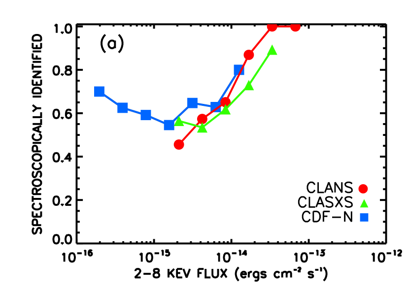
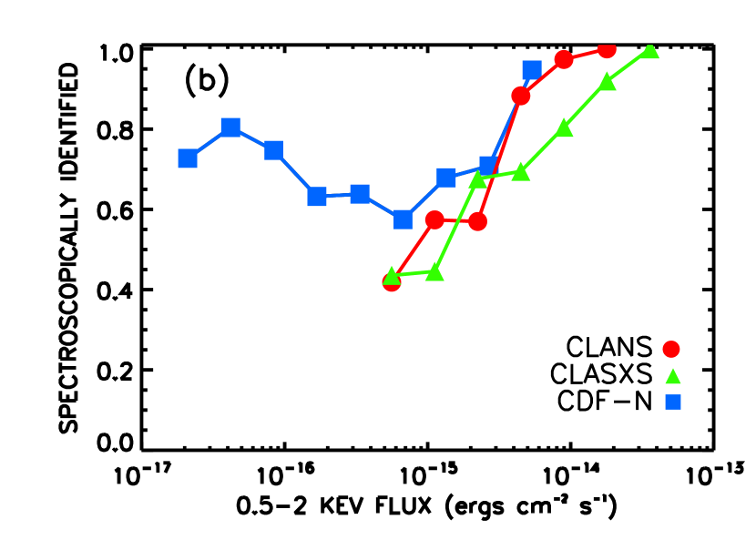
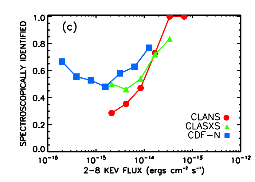
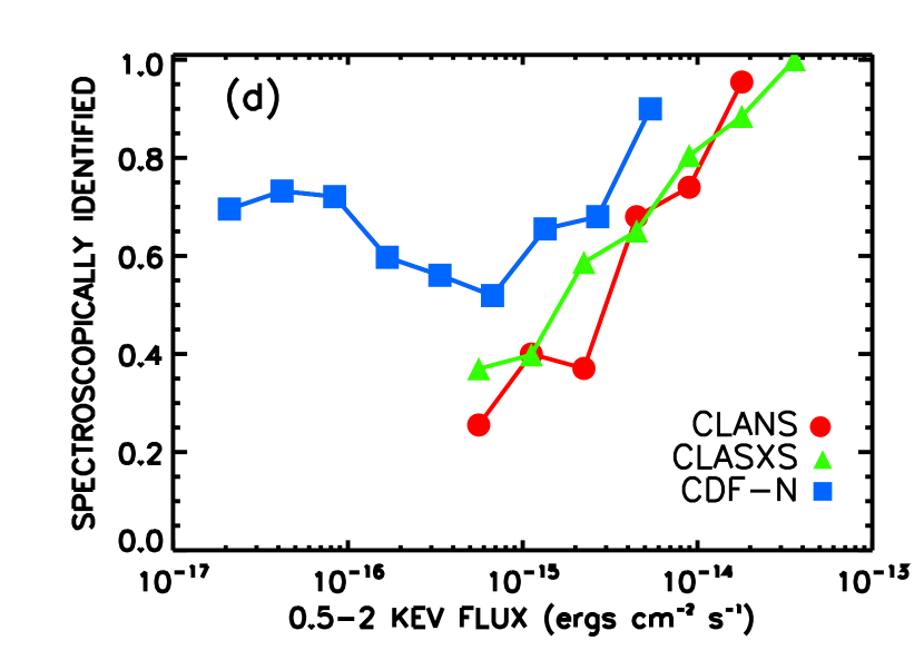
Figure 6.— (a) Fraction of spectroscopically observed sources that are spectroscopically identified in the $2-8~{}\rm keV$ band (red circles, CLANS; green triangles, CLASXS; blue squares, CDF-N). Only flux bins containing more than 10 sources are plotted. (b) Same as (a) but in the $0.5-2~{}\rm keV$ band. (c) Fraction of all sources that are spectroscopically identified in the $2-8~{}\rm keV$ band. (d) Same as (c) but in the $0.5-2~{}\rm keV$ band.

4.3. Photometric Redshifts

It is possible to extend the redshift information to fainter magnitudes using photometric redshifts. To determine photometric redshifts for the X-ray sources in the CLANS, CLASXS, and CDF-N fields, we used the template-fitting method described in Wang et al. (2006; see also Pérez-González et al. 2005). In this method one builds comparison templates using sources within the sample.

Following the prescription in Wang et al. (2006), we created SEDs for our sources using the optical through IR data to match with template SEDs. The CLANS field has 8 bands of coverage ($g^{\prime},r^{\prime},i^{\prime},z^{\prime},J,H,K,3.6~{}\mu$m), the CLASXS field has 11 bands of coverage ($u,B,g^{\prime},V,R,i^{\prime},z^{\prime},J,H,K,3.6~{}\mu$m), and the CDF-N field has 10 bands of coverage ($U,B,V,R,I,z^{\prime},J,H,K_{s},3.6~{}\mu$m). We used the $J$-band fluxes to normalize the bolometric fluxes for each source.

We then used the spectroscopically identified sources in each field to construct seven distinct templates over the frequency range from $6\times 10^{13}$ to $3\times 10^{15}$ Hz. Each template was created by taking the median $\nu f_{\nu}/\nu f_{\nu~{}(J-band)}$ values of the rest-frame SEDs with similar shapes. Figure 7 shows the templates for the CDF-N field. In this work, we have not created templates specific to each spectroscopic class, although the majority of the SEDs used to create the templates with large FUV to J-band ratios are broad-line AGNs. Trouille et al. (2008, in preparation) discuss in detail the differences between the SEDs for broad-line AGNs and for non-broad-line AGNs for our sample.

Figure 7.— CDF-N template SEDs created by taking the median $\nu f_{\nu}/\nu f_{\nu~{}(J-band)}$ values of the rest-frame SEDs with similar shapes.

Next we determined the photometric redshifts by finding the best-fit, via least-squares minimization, between our individual source SEDs and these templates. The best-fit in least-squares minimization is the one in which the sum of the squared residuals has its least value; a residual being the difference between the observed value and the template value. Sources whose best-fit corresponded to a value greater than 4.5 were not assigned a photometric redshift. This optimized the number of sources for which we could determine photometric redshifts in each field while minimizing the number of seriously discrepant sources. Throughout, we only used sources with reliable magnitude determinations in at least 4, 5, and 5 of the wavebands for the CLANS, CLASXS, and CDF-N fields, respectively.

In Figure 8 we compare our photometric redshifts ($z_{T}$) with the spectroscopic redshifts ($z_{S}$) for the spectroscopically identified sources. Of the 327, 260, and 307 spectroscopically identified sources in the CLANS, CLASXS, and CDF-N fields that are not stars, we detected 270, 223, and 296, respectively, in at least the minimum number of bands. We were able to determine photometric redshifts for $\sim 80$% of these.

Figure 8 also shows the photometric redshift residuals for each field (base panels). The dashed lines enclose the 1$\sigma$ error interval for $(z_{T}-z_{S})/(1+z_{S})$. The redshift dispersion for the combined sample is $\sigma_{z}\sim 0.16(1+z_{S})$. The redshift dispersion improves slightly to $\sigma_{z}\sim 0.11(1+z_{S})$ when only considering the absorbers in our sample and degrades to $\sigma_{z}\sim 0.2(1+z_{S})$ for the broad-line AGNs (these are marked in the figure with large open squares). The effect of this is mitigated by the fact that in our spectroscopically observed sample, the identification of the broad-line AGNs is highly complete (see §5) and so these sources generally do not require photometric redshifts. Therefore, this is only of importance to the relatively small percentage ($10-30$%) of spectroscopically unobserved sources in our three fields. With $<6$% of the sources for which we are able to determine photometric redshifts being seriously discrepant sources (i.e., having $[z_{T}-z_{S}]/[1+z_{S}]>2~{}\sigma$), the method robustly places sources in the correct redshift range.

Of the sources for which we could not determine photometric redshifts (sources whose least-squares minimization exceeded our threshold of 4.5), $\sim$50% have SEDs that lack the smoothness needed to be fit by any of our individual templates. The other $\sim$50% are smooth but have SEDs that differ too much from any of the templates to be fit by them.

Of the 425, 245, and 182 spectroscopically unidentified sources in the CLANS, CLASXS, and CDF-N fields, we detected 286, 166, and 134, respectively, in at least the minimum number of bands. Of these, we were able to determine photometric redshifts for 234, 134, and 107, respectively (i.e., again, for about 80% of them).

In order to test the reliability of our template-fitting program, we compared our CDF-N photometric redshift determinations with those we determined using the publicly available photometric redshift code HyperZ (Bolzonella et al. 2000). We used the CDF-N field because it has the highest level of spectroscopic completeness of the three fields and excellent multiwavelength coverage. HyperZ measures photometric redshifts by finding the best fit, defined by the $\chi^{2}$ statistic, to the observed SED from a library of galaxy templates. We used the eight Bruzual & Charlot (1993) templates provided with the program covering a range of galaxy types (burst, elliptical, S0, Sa, Sb, Sc, Sd, Im).

Imposing a $\chi^{2}<15$ and $P(\chi)<1$ limit appears to optimize the completeness of the HyperZ photometric redshifts while minimizing the number of seriously discrepant sources. We determined this by comparing our HyperZ photometric redshifts with our spectroscopic redshifts for the spectroscopically identified sources. The triangles in Figure 8c show the 190 HyperZ photometric redshifts for the spectroscopically identified sources in the CDF-N field. The redshift dispersion for the HyperZ results is $\sigma_{z}\sim 0.29(1+z_{S})$, as compared to $\sigma_{z}\sim 0.15(1+z_{S})$ using our template-fitting approach on the CDF-N. Restricting the sample to only broad-line AGNs, both methods exhibit a degraded goodness-of-fit. The redshift dispersion for the broad-line AGNs using HyperZ is $\sigma_{z}\sim 0.30(1+z_{S})$, as compared to $\sigma_{z}\sim 0.24(1+z_{S})$ using our template-fitting approach on the CDF-N broad-line AGNs.

Of the spectroscopically unidentified sources in the CDF-N field that were detected in at least the minimum number of bands (134), we were able to determine photometric redshifts for 75 of them using HyperZ. For comparison, we were able to determine photometric redshifts for 107 of them using our template-fitting technique.

Figure 9 shows the HyperZ photometric redshifts versus our template-fit photometric redshifts for all the sources (spectroscopically identified or unidentified) in the CDF-N for which we were able to determine photometric redshifts. The panel at the base of this figure shows the photometric redshift residuals. The dashed lines enclose the 1$\sigma$ error interval, which is $\sigma_{z}\sim 0.25(1+z_{S})$. We have overlaid open circles on the 15 $(z_{H}-z_{T})/(1+z_{T})>\sigma$ sources with known spectroscopic redshifts. For all 15 of these sources, our template-fit photometric redshifts are within $\Delta z<0.5$ of the spectroscopic redshifts. Of the remaining sources, less than 5% of the HyperZ CDF-N photometric redshifts exhibit $(z_{H}-z_{T})/(1+z_{T})>2\sigma$.

Given that our template-fitting method provides a more reliable, self-consistent, and complete photometric redshift determination method than HyperZ, we only use our template-fit photometric redshifts hereafter.

Figure 8.— Comparison of the photometric redshifts with the spectroscopic redshifts for the spectroscopically identified sample in the (a) CLANS, (b) CLASXS, and (c) CDF-N fields (open circles, our template-fitting technique results; large open squares, broad-line AGNs; filled triangles in c only, HyperZ results). The panels at the base of each figure show the photometric redshift residuals for our template-fitting results for each field. Dashed lines enclose the 1$\sigma$ error interval for $(z_{T}-z_{S})/(1+z_{S})$.

Figure 9.— Our template-fit photometric redshifts versus HyperZ photometric redshifts for all the sources (spectroscopically identified or unidentified) in the CDF-N field for which we were able to determine photometric redshifts (solid circles). Open squares indicate the broad-line AGNs. Open circles designate the 15 $(z_{H}-z_{T})/(1+z_{T})>\sigma$ outlier sources with known spectroscopic redshifts. For all 15 of these sources, our template-fit photometric redshifts are within $\Delta z<0.5$ of the spectroscopic redshifts.

4.4. Redshift and Flux Distributions

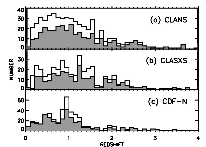
Figure 10.— Number of sources with spectroscopic (shading) and photometric (open) redshifts versus redshift for the CLANS, CLASXS, and CDF-N samples. Bin size $\Delta z=0.1$.

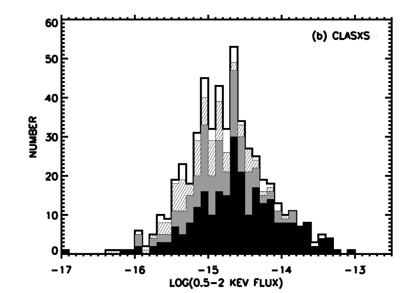
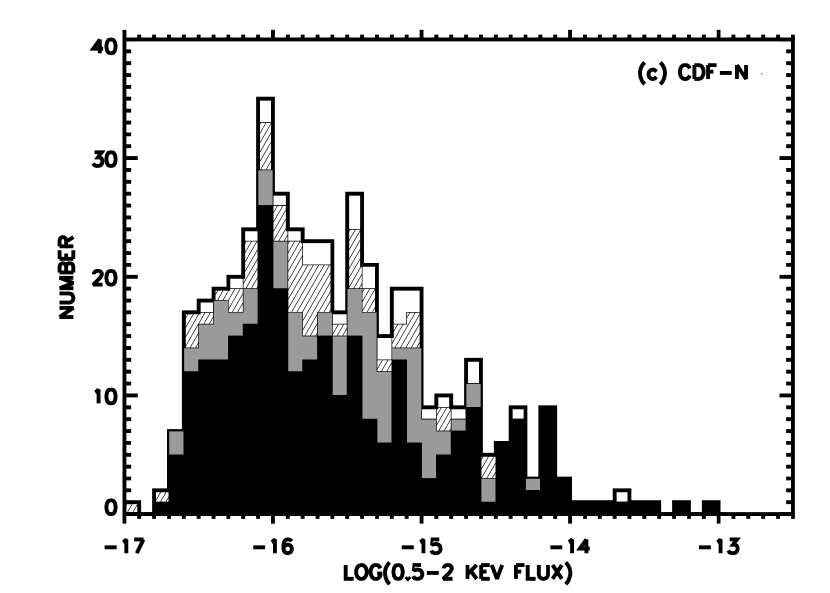
Figure 11.— $0.5-2~{}\rm{keV}$ flux distributions for the (a) CLANS, (b) CLASXS, and (c) CDF-N X-ray sources (filled, spectroscopic redshifts; shading, photometric redshifts; hatched, spectroscopically observed but unidentified and no photometric redshift determined; open, spectroscopically unobserved and no photometric redshift determined).

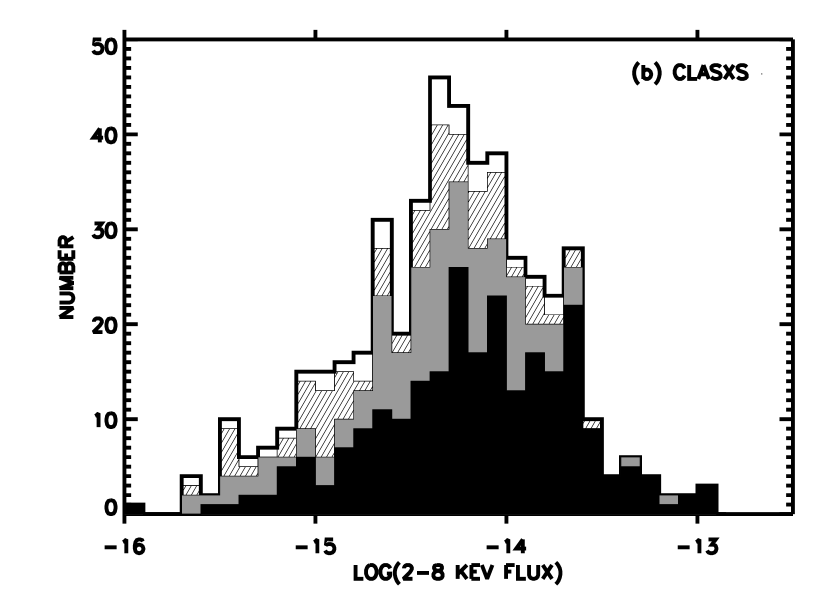
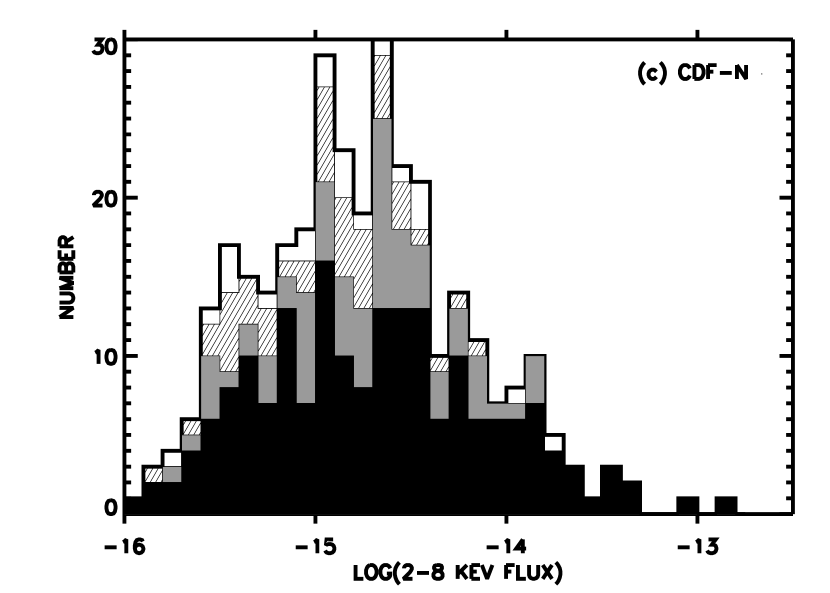
Figure 12.— $2-8~{}\rm{keV}$ flux distributions for the (a) CLANS, (b) CLASXS, and (c) CDF-N X-ray sources (filled, spectroscopic redshifts; shading, photometric redshifts; hatched, spectroscopically observed but unidentified and no photometric redshift determined; open, spectroscopically unobserved and no photometric redshift determined).

Figure 10 shows the redshift distribution of sources in the three fields with spectroscopic (shading) and photometric (open) redshifts using a low-resolution ($\Delta z=0.1)$ binning. There are no obvious structures at $z<1$ in the CLANS and CLASXS spectroscopic redshift distributions, unlike the apparent excesses found at $z=0.48$ and $0.94$ in the CDF-N sample by Barger et al. (2003) and at $z=0.674$ and $0.734$ in the CDF-S sample by Gilli et al. (2003) and Szokoly et al. (2004). There may be a grouping of CLASXS sources at $z\sim 1.2$. While there is some structure in the redshift distributions for both the CLANS and CLASXS fields, the differences between the redshift distributions for those fields versus the CDFs show that we have sampled a large enough area in the CLANS and CLASXS fields to suffer less cosmic variance compared to the CDFs.

Figures 11 and 12 show the $0.5-2~{}{\rm keV}$ and $2-8~{}{\rm keV}$ flux distributions for the CLANS, CLASXS, and CDF-N sources. The spectroscopically identified sources (filled), photometrically identified sources (shading), spectroscopically observed but neither spectroscopically nor photometrically identified sources (hatched), and spectroscopically unobserved and photometrically unidentified sources (open) are indicated. With photometric redshifts for more than $50$% of the spectroscopically unidentified sources below $10^{-14}$ ergs cm^-2 s^-1 ($2-8~{}\rm keV$), we are able to determine $2-8~{}\rm keV$ X-ray luminosities for $\sim 75$% of all the sources in the full sample (see §7).

5. OPTICAL SPECTRAL CLASSIFICATION

We have classified the spectroscopically identified Chandra sources into four optical spectral classes according to the prescription in Barger et al. (2005). We call sources without any strong emission lines [EW([OII])$<3$ Å or EW(H$\alpha$ + NII) $<10$ Å] absorbers; sources with strong Balmer lines and no broad or high-ionization lines star formers; sources with [NeV] or CIV lines or strong [OIII] [EW([OIII] $\lambda 5007)>3$EW(H$\beta$)] high-excitation sources; and, finally, sources with optical lines having FWHM line widths greater than 2000 km s^-1 broad-line AGNs. See Barger et al. (2005) for a more detailed discussion of the use of 2000 km s^-1 as the dividing line for broad-line AGNs.

In an effort to have our classifications for the sources in the three fields be as uniformly determined as possible, several of the authors repeated the classifications for all of the sources in all three fields and came to a consensus. We note that there may be some redshift bias in the classifications. Above $z\sim 0.65$, at which point MgII enters the bandpass, we can expect to have a uniform classification of broad-line AGNs, though there may be a few anomolous cases. At lower redshifts, however, there may be a number of sources classified as broad-line Seyferts which would not be identified as broad-line AGNs at high redshifts.

Table 10 gives the number of sources by optical spectral type for the CLANS, CLASXS, and CDF-N samples.

Table 10Breakdown of the X-ray Samples by Field and Spectral Class

Category	CLANS	CLASXS	CDF-N
Total	761	525	503
Observed	533	468	459
Identified	336	280	312
Broad-line	126	103	39
High-excitation	92	57	42
Star formers	87	77	146
Absorbers	22	23	71
Stars	9	20	14

6. OPTICAL/IR COUNTERPARTS CATALOGS

6.1. CLANS

In Table 11 we present the all new optical, NIR, and MIR magnitudes and spectroscopic information for the CLANS X-ray point source catalog. We ordered the 761 sources by increasing right ascension and labeled each with the Table 3 source number (col [1]). Columns (2) and (3) give the right ascension and declination coordinates of the optical/NIR counterparts in decimal degrees. Columns (4)-(10) provide the aperture-corrected, broadband $g^{\prime},r^{\prime},i^{\prime},z^{\prime},J,H,$ and $K$ magnitudes. Columns (11) and (12) give the $3.6~{}\mu$m and $24~{}\mu$m Spitzer magnitudes. Column (13) lists the spectroscopic redshifts, column (14) lists the photometric redshifts determined using our template-fitting technique, and column (15) lists the optical spectral classifications.

6.2. CLASXS

In Table 12 we present the new and updated or existing optical, NIR, and MIR magnitudes and spectroscopic information for the CLASXS X-ray point source catalog. For any source with both CFHT and Subaru data in the $R$- and $z^{\prime}$-bands, we used the CFHT magnitude. We ordered the 525 X-ray sources by increasing right ascension and labeled each with the Yang et al. (2004) source number (col [1]). Columns (2) and (3) give the right ascension and declination coordinates of the optical/NIR counterparts in decimal degrees. Columns (4)-(13) provide the new and updated aperture-corrected broadband $u,g^{\prime},B,V,R,i^{\prime},z^{\prime},J,H,$ and $K$ magnitudes. Columns (14) and (15) give the $3.6~{}\mu$m and $24~{}\mu$m Spitzer magnitudes. Column (16) lists the updated spectroscopic redshifts, column (17) lists the photometric redshifts determined using our template-fitting technique, and column (18) lists the optical spectral classifications.

6.3. CDF-N

In Table 13 we give the optical, NIR, MIR, and spectroscopic information for the CDF-N X-ray point source catalog. We ordered the 503 sources by increasing right ascension and labeled each with the Alexander et al. (2003) Table 3a source number (col [1]). Columns (2) and (3) provide the right ascension and declination coordinates of the optical/NIR counterparts in decimal degrees. Columns (4)-(9) provide the Barger et al. (2003) $U,B,V,R,I,$ and $z^{\prime}$ magnitudes (from the images of Capak et al. 2004). Columns (10)-(12) give the new $J,H,$ and $K_{s}$ magnitudes. Columns (13) and (14) give the $3.6~{}\mu$m and $24~{}\mu$m Spitzer magnitudes. Column (15) lists the updated spectroscopic redshifts, column (16) lists the photometric redshifts determined using our template-fitting technique, and column (17) lists the optical spectral classifications.

Table 11CLANS Optical/IR Counterparts Catalog

#	RA	DEC	$g^{\prime}$	$r^{\prime}$	$i^{\prime}$	$z^{\prime}$	$J$	$H$	$K$	$3.6~{}\mu$m	$24~{}\mu$m	zspec	zphot	class
(1)	(2)	(3)	(4)	(5)	(6)	(7)	(8)	(9)	(10)	(11)	(12)	(13)	(14)	(15)
1	-99.000	-99.000	-99.00	-99.00	-99.00	-99.00	-99.00	-99.00	-99.00	-99.00	-99.00	-1.00	-99.00	-1
2	160.642	59.176	23.04	22.40	21.91	21.78	21.02	19.80	-99.00	19.50	-99.00	1.43	-3.00	4
3	160.642	59.169	25.43	25.04	24.40	23.71	22.53	21.93	-99.00	-99.00	-99.00	-1.00	1.35	-1
4	-99.000	-99.000	-99.00	-99.00	-99.00	-99.00	-99.00	-99.00	-99.00	-99.00	-99.00	-1.00	-99.00	-1
5	-99.000	-99.000	-99.00	-99.00	-99.00	-99.00	-99.00	-99.00	-99.00	20.87	-99.00	-1.00	-99.00	-1
..	..	..	..	..	..	..	..	..	..	..	..	..	..	..

Table 12CLASXS Optical/IR Counterparts Catalog

#	RA	DEC	$u$	$B$	$g^{\prime}$	$V$	$R$	$i^{\prime}$	$z^{\prime}$	$J$	$H$	$K$	$3.6~{}\mu$m	$24~{}\mu$m	zspec	zphot	class
(1)	(2)	(3)	(4)	(5)	(6)	(7)	(8)	(9)	(10)	(11)	(12)	(13)	(14)	(15)	(16)	(17)	(18)
1	157.731	57.556	24.33	-99.00	23.69	-99.00	22.44	21.91	-99.00	20.17	20.30	-99.00	-1.00	-99.00	-1.00s	0.55	-1
2	157.748	57.646	-99.00	-99.00	23.74	-99.00	21.97	21.44	-99.00	20.44	20.17	-99.00	-1.00	17.84	-1.00s	0.45	-1
3	157.764	57.614	23.96	-99.00	-99.00	-99.00	22.80	22.65	-99.00	22.06	21.88	-99.00	-1.00	-99.00	0.00s	0.25	-99
4	157.774	57.630	23.80	-99.00	23.78	-99.00	23.04	22.96	23.05	22.56	-99.00	-99.00	-1.00	-99.00	0.00s	-99.00	-99
5	157.800	57.590	25.29	24.51	24.27	-99.00	23.24	22.71	22.39	21.94	21.76	-99.00	-1.00	-99.00	0.00s	0.35	-99
..	..	..	..	..	..	..	..	..	..	..	..	..	..	..	..	..	..

Table 13CDF-N Optical/IR Counterparts Catalog

#	RA	DEC	$U$	$B$	$V$	$R$	$I$	$z^{\prime}$	$J$	$H$	$K_{s}$	3.6$~{}\mu$m	24$~{}\mu$m	zspec	zphot	class
(1)	(2)	(3)	(4)	(5)	(6)	(7)	(8)	(9)	(10)	(11)	(12)	(13)	(14)	(15)	(16)	(17)
1	188.813	62.235	26.4	25.7	25.3	25.1	25.2	24.8	-99.0	-99.0	23.12	-99.00	-99.00	-1.00	-99.00	-1
2	188.820	62.261	25.4	24.9	24.9	24.5	24.7	24.5	-99.0	22.1	21.41	-99.00	-99.00	0.00a	-99.00	-99
3	188.828	62.264	21.3	20.2	19.1	18.6	18.2	18.0	17.0	16.7	16.62	-99.00	-99.00	0.14a	-3.00	0
4	188.831	62.228	27.2	26.7	25.6	24.4	23.6	23.2	-99.0	22.3	21.70	-99.00	-99.00	-1.00	0.65	-1
5	188.839	62.274	23.2	22.8	22.4	21.8	21.4	21.2	20.6	20.2	20.06	-99.00	-99.00	0.56a	-3.00	1
..	..	..	..	..	..	..	..	..	..	..	..	..	..	..	..	..

7. X-ray Luminosities

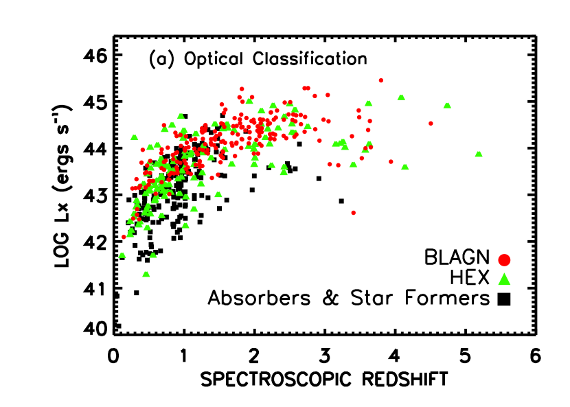
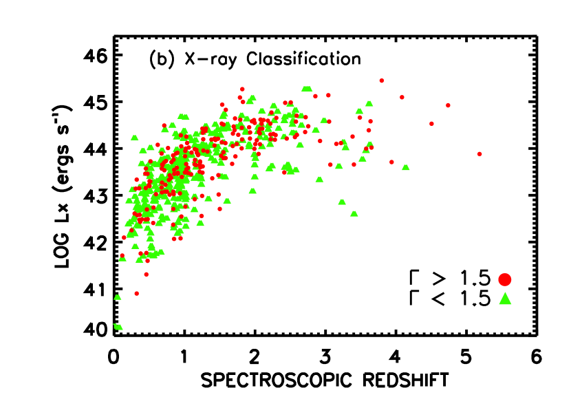
Figure 13.— (a) Rest-frame $2-8~{}\rm keV$ X-ray luminosity versus redshift for the CLANS, CLASXS, and CDF-N sources according to their optical classification (red circles, broad-line AGNs; green triangles, high-excitation narrow-line sources [HEX]; black squares, absorbers and star formers). We only include sources with spectroscopic redshifts, $L_{X}>10^{40}$ ergs s^-1, and an X-ray detection significance greater than $3\sigma$. (b) Same as (a) but now classifying the sources according to their X-ray spectral properties (red circles, $\Gamma>1.5$; green triangles, $\Gamma<1.5$).

We used the X-ray fluxes and redshifts of our sources to calculate their rest-frame $2-8~{}\rm keV$ X-ray luminosities. We limited our sample to sources with an X-ray detection significance greater than $3\sigma$. For the CLANS sources we determined the $3\sigma$ significance level using the $1\sigma$ error bars on the $2-8~{}\rm keV$ and $0.5-2~{}\rm keV$ flux values listed in Table 4. For the CLASXS and CDF-N sources we used the $1\sigma$ error bars from Yang et al. (2004) and Alexander et al. (2003), respectively.

At $z<3$, we calculated the luminosities from the observed-frame $2-8~{}\rm keV$ fluxes, and at $z>3$, we used the observed-frame $0.5-2$ keV fluxes. One advantage of using the observed-frame $0.5-2~{}\rm keV$ X-ray fluxes at high redshifts is the increased sensitivity, since the $0.5-2~{}\rm keV$ Chandra images are deeper than the $2-8~{}\rm keV$ images. In addition, at $z=3$, observed-frame $0.5-2~{}\rm keV$ corresponds to rest-frame $2-8~{}\rm keV$, providing the best possible match to the lower redshift data.

In calculating the $K-$corrections for obtaining the rest-frame $2-8~{}\rm keV$ luminosities, we assumed an intrinsic $\Gamma=1.8$. Since the $K-$correction factor for emission modeled by a power law follows the form $[1+z]^{\Gamma-2}$, these corrections are very small. If we instead assumed the individual photon indices used in the flux calculations (rather than the universal power-law index of $\Gamma=1.8$ adopted here) to calculate the $K-$corrections, we would find only a small difference in the rest-frame luminosities (Barger et al. 2002).

In short, the rest-frame $2-8~{}\rm keV$ luminosity, $L_{X}$, equals $f\times 4\pi d_{L}^{2}\times K-$correction.

$$\hskip 4.2679ptz<3:\hskip 5.69054ptK-{\rm corr.}=(1+z)^{-0.2}\hskip 5.69054pt{\rm\&}\hskip 5.69054ptf=f_{2-8~{}{\rm keV}}$$ (4)

$$z\geq 3:\hskip 5.69054ptK-{\rm corr.}=\frac{1}{4}(1+z)^{-0.2}\hskip 5.69054pt{\rm\&}\hskip 5.69054ptf=f_{0.5-2~{}{\rm keV}}$$ (5)

The $\frac{1}{4}$ factor in the $z\geq 3$ $K-$correction is a result of normalizing so that there is no $K-$correction if $z=3$, when the observed-frame $0.5-2$ keV corresponds exactly to the rest-frame $2-8$ keV.

Figure 13a shows rest-frame $2-8~{}\rm keV$ X-ray luminosity versus spectroscopic redshift for the CLANS, CLASXS, and CDF-N X-ray sources split by their optical spectral classification. This figure illustrates the Steffen effect, in which the broad-line AGNs dominate the number densities at higher X-ray luminosities, while the non-broad-line AGNs dominate at lower X-ray luminosities (Steffen et al. 2003).

Figure 13b shows the same relation, but now the sources in the three fields are split by their X-ray classifications. For the CLANS and CLASXS X-ray sources, we converted the individual hardness ratios, HR, into $\Gamma$ values, as described in §2.2. For the CDF-N X-ray sources, we used the Alexander et al. (2003) values for $\Gamma$. We note that $\sim 1/4$ of the sources in Figure 13b are within $1\sigma$ of $\Gamma=1.5$.

Figures 13a and 13b demonstrate that while the optical and X-ray classifications show generally the same broad differentiation between the classes, there is clearly a different scatter or mixing of the objects, which reflects the properties of each individual source. In Yencho et al. (2008) we present the X-ray luminosity functions by spectral type, and in L. Trouille et al. (2008, in preparation) we present a detailed analysis of the optical and X-ray spectral characteristics of the individual objects in our sample.

8. NUMBER COUNTS

In order to determine the amount of field to field variation within our sample and to compare our survey with those by others, we have determined the differential number counts for each individual field and for the full sample.

In the following, we have excluded any CLANS or CLASXS sources with off-axis angles greater than $8\arcmin$ because the sensitivity of Chandra drops significantly at large off-axis angles and because of the field overlap in the CLASXS region. Using the Yang et al. (2006) simulations (see §2.5), we have also excluded any CLANS and CLASXS sources with fluxes less than the flux threshold for the source’s particular off-axis angle location and pointing exposure time (see Figure 3). In this section, we use only the flux thresholds and $\Omega(S_{i})$ values for a 30% probability of detection. See §2.5 and Figure 5 for a discussion of the $\Omega(S_{i})$ values used for the CLANS and CLASXS fields.

The Poisson fluctuations in the source fluxes could result in an overestimation of the number counts close to the detection limits. This is known as the Eddington bias. For the CLANS and CLASXS fields, the detection threshold is below the ‘knee’ of the log$N-$log$S$ relation, and the Eddington bias is relatively small. We have not included the Eddington bias correction in our determination of the number counts for these fields (including the Eddington bias correction from the Yang et al. 2004 simulations does not change the results significantly).

We used the Alexander et al. (2003) $\Omega(S_{i})$ values (see their Figure 19) and flux threshold values for the CDF-N field. We also applied the Bauer et al. (2004) recovered flux corrections (see their Figure 2) to account for the few percent increase at all fluxes due to an additional aperture correction not originally accounted for in Alexander et al. (2003), an increase for faint sources due to photometry errors (see their Figure 3), and a decrease for faint sources due to the Eddington bias. In the following, we have excluded any CDF-N sources with off-axis angles greater than $10\arcmin$ as well as any CDF-N sources with fluxes less than the flux threshold for the source’s particular off-axis angle location.

We computed the differential log$N-$log$S$ relations for the full and individual samples using the formula

$$\frac{dN}{dS}=\sum_{S_{1}<S_{i}<S_{2}}\frac{1}{\Omega_{tot}(S_{i})\times\Delta S}$$ (6)

in units of deg^-2 per 10^-15 ergs cm^-2 s^-1. $S_{1}$ and $S_{2}$ are the minimum and maximum fluxes in each bin. $\Delta S=S_{2}-S_{1}$. We estimated the error bars in the number counts by the error propagation rule using Gehrels (1986) statistics.

Figure 14 shows the (a) $0.5-2~{}\rm keV$ and (b) $2-8~{}\rm keV$ differential number counts for the full sample, as well as for each field individually. The bottom plots compare the differential number counts for our full sample with those from other surveys. We parametrized our best-fits to the full sample, shown as black dashed lines in the plots, by means of a broken power law of the form

$$dN/dS=n_{0,faint}(S/10^{-14})^{-\alpha_{faint}}\hskip 14.22636pt(S<S_{break})\\$$ (7)

$$\hskip 34.1433pt=n_{0,bright}(S/10^{-14})^{-\alpha_{bright}}\hskip 11.38109pt(S>S_{break})$$ (8)

We determined the best-fits using error-weighted least-squares fits. Table 14 shows the best-fit parameters. The quoted errors are 1$\sigma$ formal errors on the fits.

Figure 15 shows the (a) $0.5-2~{}\rm keV$ and (b) $2-8~{}\rm keV$ differential number counts fractional residuals for each field separately, defined as 1 minus the ratio of $dN/dS$ for the individual sample and $dN/dS$ for the full sample. The fields agree reasonably well, exhibiting a variance of $<10\%$ in almost all of the $0.5-2~{}\rm keV$ and $2-8~{}\rm keV$ flux bins.

In Figure 16 we directly compare the best-fit slopes for the (a) $0.5-2~{}\rm keV$ and (b) $2-8~{}\rm keV$ faint and bright ends of our differential number counts with those of other surveys (see Kim et al. 2007b for an exhaustive comparison of differential number counts determinations from surveys to date). The best-fit slopes of $1.48\pm 0.02$ and $1.64\pm 0.02$, respectively, for the faint end of our full sample $0.5-2~{}\rm keV$ and $2-8~{}\rm keV$ band differential number counts agree well with other surveys. However, we note that our results at the faint end are not independent from the Kim et al. (2007b) and Cowie et al. (2002) results (points 4 and 6 in Figure 16), since these also include the CDF-N. At the bright end, our uncertainties are larger. However, the $0.5-2~{}\rm keV$ band differential number counts best-fit slope of $2.0\pm 0.3$ is within the errors of the other surveys (note that the Yang et al. 2004 slope was fixed at 2.5 with no error). The actual value of the slope is slightly shallower than that of the other surveys. In the $2-8~{}\rm keV$ band, the best-fit slope of $2.7\pm 0.5$ agrees reasonably well with the results from other surveys.

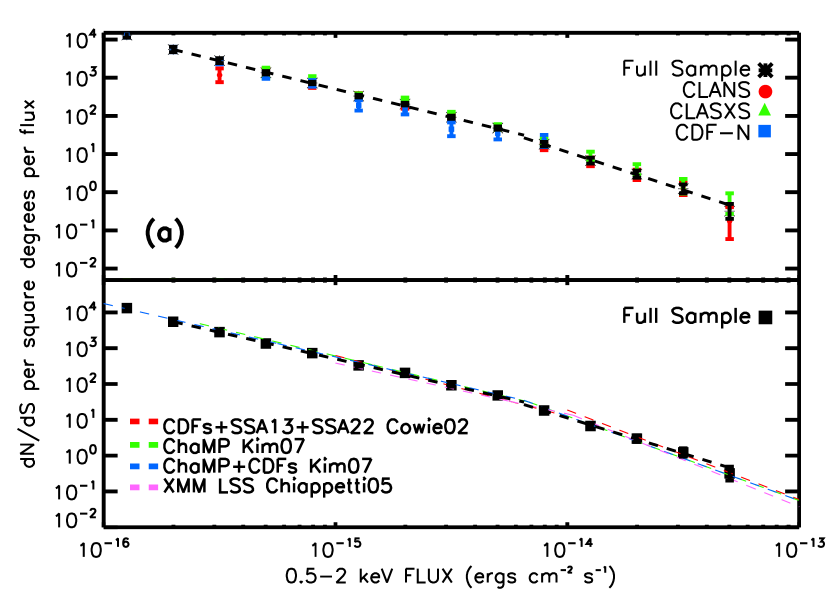
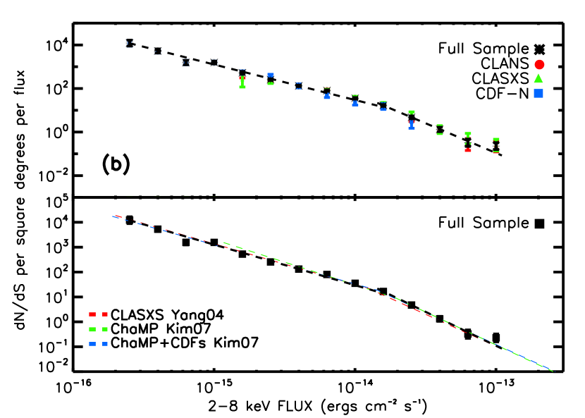
Figure 14.— (a) $0.5-2~{}\rm keV$ band differential number counts (black asterix, full sample; red circles, CLANS; green triangles, CLASXS; blue squares, CDF-N; black dashed line, best-fit to the full sample). Only results for bins with at least four sources are shown. Bottom plot in (a) shows the full sample (black squares) overplotted with results from other surveys, as indicated. (b) Same as (a) but for the $2-8~{}\rm keV$ band differential number counts.

Table 14Broken Power Law Best-fit Parameters for the Full Sample

Diff. Num. Counts	Faint End		Break Flux	Bright End
	$n_{0}$	$\alpha$		$n_{0}$	$\alpha$
$0.5-2~{}\rm keV$	$16.5\pm 1.2$	$1.48\pm 0.02$	$6.5\times 10^{-15}$	$11.3\pm 0.4$	$2.0\pm 0.3$
$2-8~{}\rm keV$	$29.7\pm 1.2$	$1.64\pm 0.02$	$1.44\times 10^{-14}$	$59.0\pm 27.0$	$2.7\pm 0.5$

Figure 15.— $0.5-2~{}\rm keV$ and $2-8~{}\rm keV$ band differential number count residuals, defined as 1 minus the ratio of $dN/dS$ for the individual sample and $dN/dS$ for the full sample, for the CLANS, CLASXS, and CDF-N fields. Only results for bins with at least four sources are shown.

Figure 16.— (Top) Faint and (bottom) bright power indices of the differential number counts for this and previous studies in (a) the $0.5-2~{}\rm keV$ band and (b) the $2-8~{}\rm keV$ band. The references are as follows: (1) this study; (2) Yang et al. (2004) CLASXS; (3) Chiappetti et al. (2005) XMM LSS; (4) Kim et al. (2007b) ChaMP+CDFs; (5) Kim et al. (2007b) ChaMP; (6) Cowie et al. (2002) CDFs+SSA13+SSA22. Note that Yang et al. (2004) fixed the bright slope as 2.5 in the $0.5-2~{}\rm keV$ band, so there is no error.

9. SUMMARY

In this paper, we compiled the database for the OPTX project, which combines data from the CLANS, CLASXS, and CDF-N fields to create one of the most spectroscopically complete samples of Chandra X-ray sources to date. With this database, we can analyze the effect of spectral type on the shape and evolution of the X-ray luminosity functions and compare the optical and X-ray spectral properties of the X-ray sources in our sample.

In detail, we presented the first X-ray, infrared, and optical photometric and spectroscopic catalogs for the CLANS field. The CLANS X-ray survey covers 0.6 deg² and reaches fluxes of $7\times 10^{-16}$ ergs cm^-2 s^-1 in the $0.5-2~{}\rm keV$ band and $3.5\times 10^{-15}$ ergs cm^-2 s^-1 in the $2-8~{}\rm keV$ band. We presented $g^{\prime},r^{\prime},i^{\prime},z^{\prime},J,H,K,3.6~{}\mu$m, and $24~{}\mu$m photometry for the 761 X-ray sources in the sample. We spectroscopically observed 533 of the CLANS sources, obtaining redshift identifications for 336. We extended the redshift information to fainter magnitudes using photometric redshifts, which resulted in an additional 234 redshifts.

We also presented new and updated CLASXS photometry and some new spectroscopy, along with existing data. Using new $u,g^{\prime},$ and $i^{\prime}$ magnitudes, we corrected the zeropoints for the original Steffen et al. (2004) $V,R,I,$ and $z^{\prime}$ photometry (the $B$-band zeropoint was fine). We also obtained $J,H,K,3.6~{}\mu$m, and $24~{}\mu$m photometry for the 525 X-ray sources in the sample. Since the publication of the Steffen et al. (2004) redshift catalog for this field, we have obtained an additional 11 spectra and identified redshifts for all 11. As a result, of the now 468 spectroscopically observed CLASXS sources, we have presented redshift identifications for 280. We extended the redshift information for the CLASXS field to include an additional 134 photometric redshifts.

Furthermore, we presented new CDF-N $J,H,$ and $K_{s}$ photometry and some new optical spectroscopy, along with existing data. We also included the GOODS-N Spitzer $3.6~{}\mu$m and $24~{}\mu$m detections. Since the publication of the Barger et al. (2003) redshift catalog for this field, we have obtained an additional 49 spectra and identified redshifts for 39. As a result, of the 503 X-ray sources in the CDF-N field, we have spectroscopically observed 459, obtaining redshift identifications for 312. We extended the redshift information for the CDF-N field to include an additional 107 photometric redshifts.

Finally, we determined the differential X-ray number counts for each survey individually and for the full sample. Our differential number counts for the combined sample agree well with the results from other X-ray surveys.

References

- Alexander et al. (2003) Alexander, D. M., et al. 2003, AJ, 126, 539
- Alonso-Herrero et al. (1997) Alonso-Herrero, A., Ward, M. J., & Kotilainen, J. K. 1997, MNRAS, 288, 977
- Aune et al. (2003) Aune S., et al. 2003, Proc. SPIE, 4841, 513
- Barden et al. (1994) Barden, S. C., Armandroff, T., Muller, G., Rudeen, A. C., Lewis, J., & Groves, L. 1994, Proc. SPIE, 2198, 87
- Barger et al. (2002) Barger, A. J., Cowie, L. L., Brandt, W. N., Capak, P., Garmire, G. P., Hornschemeier, A. E., Steffen, A. T., & Wehner, E. H. 2002, AJ, 124, 1839
- Barger et al. (2003) Barger, A. J., et al. 2003, AJ, 126, 632
- Barger et al. (2005) Barger, A. J., Cowie, L. L., Mushotzky, R. F., Yang, Y., Wang, W., Steffen, A. T., & Capak, P. 2005, AJ, 129, 578
- Barger et al. (2008) Barger, A. J., Cowie, L. L., & Wang, W.-H. 2008, ApJ, in press
- Bauer et al. (2004) Bauer, F. E., Alexander, D. M., Brandt, W. M., Schneider, D. P., Triester, E., Hornschemeier, A. E., & Garmire, G. P. 2004, AJ, 128, 2048
- Bertin & Arnouts (1996) Bertin, E., & Arnouts, S. 1996, A&AS, 117, 393
- Bolzonella et al. (2000) Bolzonella, M., Miralles, J.-M., & Pello, R. 2000, A&A, 363, 476
- Boulade et al. (2003) Boulade, O., et al. 2003, Proc. SPIE, 4841, 72
- Brandt et al. (2001) Brandt, W. N., et al. 2001, AJ, 122, 2810
- Brandt & Hasinger (2005) Brandt, W.N., & Hasinger, G. 2005, ARA&A, 43, 829
- Bruzual & Charlot (1993) Bruzual, G. & Charlot, S. 1993, ApJ, 405, 538
- Bundy et al. (2008) Bundy, K., et al. 2008, ApJ, in press
- Capak et al. (2004) Capak, P., et al. 2004, AJ, 127, 180
- Cappelluti et al. (2007) Cappelluti, N., et al. 2007, ApJS, 172, 341
- Chapman et al. (2005) Chapman S. C., Blan, A. W., Smail, I., & Ivison, R. J. 2005, ApJ, 622, 772
- Chiappeti et al. (2005) Chiappetti, L., et al. 2005, A&A, 439, 413
- Churazov et al. (2007) Churazov, E., et al. 2007, A&A, 467, 529
- Cowie et al. (1996) Cowie, L. L., Songaila, A., Hu, E. M., & Cohen, J. G. 1996, AJ, 112, 839
- Cowie et al. (2002) Cowie, L. L., Garmire, G. P., Bautz, M. W., Barger, A. J., Brandt, W. N., & Hornschemeier, A. E. 2002, ApJ, 566, L5
- Davis et al. (2003) Davis, M., et al. 2003, Proc. SPIE, 4834, 161
- Davis et al. (2007) Davis, M., et al. 2007, ApJ, 660, 1
- Dye et al. (2006) Dye., S., et al. 2006, MNRAS, 372, 1227
- Eckart et al. (2006) Eckart, M. E., Stern, D., Helfand, D. J., Harrison, F. A., Mao, P. H., & Yost, S. A. 2006, A&A, 450, 535
- Faber et al. (2003) Faber, S. M., et al. 2003, Proc. SPIE, 4841, 1657
- Freeman et al. (2002) Freeman, P. E., Kashyap, V., Rosner, R., & Lamb, D. Q. 2002, ApJS, 138, 185
- Frontera et al. (2007) Frontera, F., et al. 2007, ApJ, 666, 86
- Gehrels (1986) Gehrels, N. 1986, ApJ, 303, 336
- Georgakakis (07) Georgakakis, A., et al. 2007, ApJ, 660, L15
- Giacconi et al. (2002) Giacconi, R., et al. 2002, ApJS, 139, 369
- Gilli et al. (2003) Gilli, R., et al. 2003, ApJ, 592, 721
- Gilli et al. (2007) Gilli, R., Comastri, A., & Hasinger, G. 2007, A&A, 463, 79
- Harrison et al. (2003) Harrison, F., Eckart, M. E., Mao, P. H., Helfand, D. J., & Stern, D. 2003, ApJ, 596, 944
- (37) Kim, M., et al. 2007a, ApJS, 169, 401
- (38) Kim, M., Wilkes, B. J., Kim, D-W., Green, P. J., Barkhouse, W. A., Lee, M. G., Silverman, J. D., & Tananbaum, H. D. 2007b, ApJ, 659, 29
- Lehmer et al. (2005) Lehmer, B. D., et al. 2005, ApJS, 161, L21
- Lockman et al. (1986) Lockman, F. J., Jahoda, K., & McCammon, D., 1986, ApJ, 302, 432
- Lonsdale et al. (2003) Lonsdale, C. J., et al. 2003, PASP, 115, 897
- Lonsdale et al. (2004) Lonsdale, C. J., et al. 2004, ApJS, 154, 54
- Loose et al. (2003) Loose, M., Farris, M. C., Garnett, J. D., Hall, D. N. B., & Kozlowski, L. J. 2003, Proc. SPIE, 4850, 867
- Magnier & Cuillandre (2004) Magnier, E. A., & Cuillandre, J.-C. 2004, PASP, 116, 449
- Monet et al. (2003) Monet, D., et al. 2003, AJ, 125, 984
- Mulchaey et al. (1994) Mulchaey, J. S., Koratkar, A., Ward, M. J., Wilson, A. S., Whittle, M., Antonucci, R., Kinney, A. L., & Hurt, T. 1994, ApJ, 436, 586
- Muno et al. (2003) Muno, M. P., et al. 2003, ApJ, 589, 225
- Murray et al. (2005) Murray S. S., et al. 2005, ApJS, 161, 1
- Nandra et al. (2005) Nandra, K., Adelberger, K., Gardner, J. P., Mushotzky, R. F., Rhodes, J., Steidel, C. C., Teplitz, H. I., Arnaud, K. A. 2005, MNRAS, 356, 568
- Oke et al. (1995) Oke, J. B., et al. 1995, PASP, 107, 375
- Polletta et al. (2006) Polletta, M., et al. 2006, ApJ, 642, 673
- Pérez-González et al. (2005) Pérez-González, P. G., et al. 2005, ApJ, 630, 82
- Reddy et al. (2006) Reddy, N. A., Steidel, C., Erb, D. K., Shapley, A. E., & Pettini, M. 2006, ApJ, 653, 1004
- Rowan-Robinson et al. (2008) Rowan-Robinson, M., et al. 2008, MNRAS, 386, 697
- Silverman et al. (2008) Silverman, J. D., et al. 2008, ApJ, 675, 1025
- Stark et al. (1992) Stark, A. A., Gammie, C. F., Wilson, R. W., Bally, J., Linke, R. A., Heiles, C., & Hurwitz, M. 1992, ApJS, 79, 77
- Steffen et al. (2003) Steffen, A. T., Barger, A. J., Cowie, L. L., Mushotzky, R. F., & Yang, Y. 2003, ApJ, 596, L23
- Steffen et al. (2004) Steffen, A. T., Barger, A. J., Capak, P., Cowie, L. L., Mushotzky, R. F., & Yang, Y. 2004, AJ, 128, 1483
- Swinbank et al. (2004) Swinbank, A. M., Smail, I., Chapman, S. C., Blain, A. W., Ivison, R. J., & Keel, W. C. 2004, ApJ, 617, 64
- Szokoly et al. (2004) Szokoly, G. P., et al. 2004, ApJS, 155, 271
- Ueda et al. (1999) Ueda, Y., Takahashi, T., Ohashi, T., & Makishima, K. 1999, ApJ, 524, L11
- Virani et al. (2006) Virani, S. N., Treister, E., Urry, M., & Gawiser, E. 2006a, AJ, 131, 2373
- (63) Virani, S. N., et al. 2006b, in Proceedings of the X-ray Universe, Ed. A. Wilson (Madrid: El Escorial), 849
- Wang et al. (2006) Wang, W., Cowie, L. L., & Barger, A. J. 2006, ApJ, 647, 74
- Yang et al. (2004) Yang, Y., Mushotzky, R. F., Steffen, A. T., Barger, A. J., & Cowie, L. L. 2004, AJ, 128, 1501
- Yang et al. (2006) Yang, Y., Mushotzky, R. F., Barger, A. J., & Cowie, L. L. 2006, ApJ, 645, 68
- Yencho et al. (2008) Yencho, B., Barger, A. J., Trouille, L., & Winter, L. M. 2008, ApJ, submitted