Distributed Constrained Optimization with Semicoordinate Transformations

Abstract

Recent work has shown how information theory extends conventional full-rationality game theory to allow bounded rational agents. The associated mathematical framework can be used to solve constrained optimization problems. This is done by translating the problem into an iterated game, where each agent controls a different variable of the problem, so that the joint probability distribution across the agents’ moves gives an expected value of the objective function. The dynamics of the agents is designed to minimize a Lagrangian function of that joint distribution. Here we illustrate how the updating of the Lagrange parameters in the Lagrangian is a form of automated annealing, which focuses the joint distribution more and more tightly about the joint moves that optimize the objective function. We then investigate the use of “semicoordinate” variable transformations. These separate the joint state of the agents from the variables of the optimization problem, with the two connected by an onto mapping. We present experiments illustrating the ability of such transformations to facilitate optimization. We focus on the special kind of transformation in which the statistically independent states of the agents induces a mixture distribution over the optimization variables. Computer experiment illustrate this for $k$-sat constraint satisfaction problems and for unconstrained minimization of $NK$ functions.

Subject Classification: programming: nonlinear, algorithms, theory; probability: applications

Area of Review: optimization

1 Introduction

1.1 Distributed optimization and control with Probability Collectives

As first described in [wolp03b, wolp04a], it turns out that one can translate many of the concepts from statistical physics, game theory, distributed optimization and distributed control into one another. This translation is based on the fact that those concepts all involve distributed systems in which the random variables are, at any single instant, statistically independent. (What is coupled is instead the distributions of those variables.) Using this translation, one can transfer theory and techniques between those fields, creating a large common mathematics that connects them. This common mathematics is known as Probability Collectives (PC). Its unifying concern is the set of probability distributions that govern any particular distributed system, and how to manipulate those distributions to optimize one or more objective functions. See [wotu03a, wotu01a] for earlier, less formal work on this topic.

In this paper we consider the use of PC to solve constrained optimization and/or control problems. Reflecting the focus of PC on distributed systems, its use for such problems is particularly appropriate when the variables in the collective are spread across many physically separated agents with limited inter-agent communication (e.g., in a distributed design or supply chain application, or distributed control). A general advantage of PC for such problems is that since they work with probabilities rather than the underlying variables, they can be implemented for arbitrary types of the underlying variables. This same characteristic also means they provides multiple solutions, each of which is robust, along with sensitivity information concerning those solutions. An advantage particulary relevant to optimization is that the distributed PC algorithm can often be implemented on a parallel computer. An advantage particularly relevant to control problems is that PC algorithms can, if desired, be used without any modelling assumptions about the (stochastic) system being controlled. These advantages are discussed in more detail below.

1.2 The Probability Collectives Approach

Broadly speaking, the PC approach to optimization/control is as follows. First one maps the provided problem into a multi-agent collective. In the simplest version of this process one assigns a separate agent of the collective to determine the value of each of the variables $x_{i}\in\mathcal{X}_{i}$ in the problem that we control. So for example if the $i$’th variable can only take on a finite number of values, those $|\mathcal{X}_{i}|$ possible values constitute the possible moves of the $i$’th agent. The value of the joint set of $n$ variables (agents) describing the system is then $\mathbf{x}=[x_{1},\cdots,x_{n}]\in\mathcal{X}$ with $\mathcal{X}\triangleq\mathcal{X}_{1}\times\cdots\times\mathcal{X}_{n}$.

Unlike many optimization methods, in PC the variables are not manipulated directly. Rather a probability distribution is what is manipulated. To avoid combinatorial explosions as the number of dimensions of $\mathcal{X}$ grows, we must restrict attention to a low-dimensional subset of the space of all probability distributions. We indicate this by writing our distributions as $q\in\cal{Q}$ over $\mathcal{X}$. The manipulation of that $q$ proceeds through an iterative process. The ultimate goal of this process is to induce a distribution that is highly peaked about the $\mathbf{x}$ optimizing the objective function $G(\mathbf{x})$, sometimes called the world cost or world utility function. (In this paper we only consider problems with a single overall objective function, and we arbitrarily choose lower values to be better, even when using the term “utility”.)

In the precise algorithms investigated here, at the start of any iteration a single Lagrangian function of $q$, $\mathcal{L}:\mathcal{Q}\rightarrow\mathbb{R}$, is specified, based on $G(\mathbf{x})$ and the associated constraints of the optimization problem. Rather than minimize the objective function over the space $\mathcal{X}$, the algorithm minimizes that Lagrangian over $q\in\mathcal{Q}$. This is done by direct manipulation of the components of $q$ by the agents.

After such a minimization of a Lagrangian, one modifies the Lagrangian slightly. This is done so that the $q$ optimizing the new Lagrangian is more tightly concentrated about $\mathbf{x}$ that solve our optimization problem than is the current $q$. One then uses the current $q$ as the starting point for another process of having the agents minimize a Lagrangian, this time having them work on that new Lagrangian.

At the end of a sequence of such iterations one ends up with a final $q$. That $q$ is then used to determine a final answer in $\mathcal{X}$, e.g., by sampling $q$, evaluating its mode, evaluating its mean (if that is defined), etc. For a properly chosen sequence of Lagrangians and algorithm for minimizing the Lagrangians, this last step should, with high probability, provide the desired optimal point in $\mathcal{X}$.

For the class of Lagrangians used in this paper, the sequence of minimizations of Lagrangians is closely related to simulated annealing. The difference is that in simulated annealing an inefficient Metropolis sampling process is used to implicitly descend each iteration’s Lagrangian. By explicitly manipulating $q$, PC allows for more efficient descent.

In this paper we shall consider the case where $\cal{Q}$ is a product space, $q(\mathbf{x})=\prod_{i}q_{i}(x_{i})$. The associated formulation of PC is sometimes called “Product Distribution” theory. It corresponds to noncooperative game theory, with each $q_{i}$ being agent $i$’s “mixed strategy” [wolp04a, futi91]. Our particular focus is the use of such product distributions when $\mathcal{X}$ is not the same as the ultimate space of the optimization variables, $\cal{Z}$. In this formulation — a modification of what was presented above — there is an intermediate mapping from $\cal{X}\rightarrow\cal{Z}$, and the provided $G$ is actually a function over $\cal{Z}$, not (directly) over $\cal{X}$. Such intermediate mappings are called “semicoordinate systems”, and going from one to another is a “semicoordinate transformation”. As elaborated below, such transformations allow arbitrary coupling among the variables in $\cal{Z}$ while preserving many of the computational advantages of using product distributions over $\cal{X}$.

1.3 Advantages of Probability Collectives

There are many advantages to working with distribution in $\mathcal{Q}$ rather than points in $\mathcal{X}$. Usually the support of $q$ is all of $\mathcal{X}$, i.e., the $q$ minimizing the Lagrangian lies in the interior of the unit simplices giving $\mathcal{Q}$. Conversely, any element of $\mathcal{X}$ can be viewed as a probability distribution on the edge (a vertex) of those simplices. So working with $\mathcal{X}$ is a special case of working with $\mathcal{Q}$, where one sticks to the vertices of $\cal{Q}$. In this, optimizing over $\mathcal{Q}$ rather than $\mathcal{X}$ is analogous to interior point methods. Due to the breadth of the support of $q$, minimizing over it can also be viewed as a way to allow information from the value of the objective function at all ${\bf{x}}\in{\mathcal{X}}$ to be exploited simultaneously.

Another advantage, alluded to above, is that by working with distributions $\mathcal{Q}$ rather than the space $\mathcal{X}$, the same general PC approach can be used for essentially any $\mathcal{X}$, be it continuous, discrete, time-extended, mixtures of these, etc. (Formally, those different spaces just correspond to different probability measures, as far as PC is concerned.) For expository simplicity though, here we will work with finite $\mathcal{X}$, and therefore have probability distributions rather than density functions, sums rather than integrals, etc. See in particular [biwo04a, wobi04b, wolp04g, wost06] for analysis explicitly for the case of infinite $\mathcal{X}$.

Yet another advantage arises from the fact that when $\mathcal{X}$ is finite, $q\in\mathcal{Q}$ is a vector in a Euclidean space. Accordingly the Lagrangian we are minimizing is a real-valued function of a Euclidean vector. This means PC allows us to leverage the power of descent schemes for continuous spaces like gradient descent or Newton’s method — even if $\mathcal{X}$ is a categorical, finite space. So with PC, schemes like “gradient descent for categorical variables” are perfectly well-defined.

While the Lagrangians can be based on prior knowledge or modelling assumptions concerning the problem, they need not be. Nor does optimization of a Lagrangian require control of all variables $\mathcal{X}$ (i.e., some of the variables can be noisy). This allows PC to be very broadly applicable.

1.4 Connection with other sciences

A more general advantage of PC is how it relates seemingly disparate disciplines to one another. In particular, it can be motivated by using information theory to relate bounded rational game theory to statistical physics [wolp03b, wolp04a]. This allows techniques from one field to be imported into the other field. For example, as illustrated below, the grand canonical ensemble of physics can be imported into noncooperative game theory to analyze games having stochastic numbers of the players of various types.

To review, a noncooperative game consists of a sequence of stages. At the beginning of each stage every agent (aka “player”) sets a probability distribution (its “mixed strategy”) over its moves [futi91, auha92, baol99, fule98]. The joint move at the stage is then formed by agents simultaneously sampling their mixed strategies at that stage. So the moves those agents make at any particular stage of the game are statistically independent and the distribution of the joint-moves at any stage is a product distribution — just like in PC theory.

This does not mean that the moves of the agents across all time are statistically independent however. At each stage of the game each agent will set its mixed strategy based on information gleaned from preceding stages, information that in general will reflect the earlier moves of the other agents. So the agents are coupled indirectly, across time, via the updating of the $\{q_{i}\}_{i=1}^{n}$ at the end of each stage.

Analogously, consider again the iterative PC algorithm outlined above, and in particular the process of optimizing the Lagrangian within some particular single iteration. Typically that process proceeds by successively modifying $q$ across a sequence of timesteps. In each of those timesteps $q({\mathbf{x}})=\prod_{i}q_{i}({x}_{i})$ is first sampled, and then it is updated based on all previous samples. So just like in a noncooperative game there is no direct coupling of the values of the underlying variables {${x}_{i}$}at any particular timestep ($q$ is a product distribution). Rather just like in a noncooperative game, the variables are indirectly coupled, across time (i.e., across timesteps of the optimization), via coupling of the distributions $q_{i}(x_{i})$ at different timesteps.

In addition, information theory can be used to show that the bounded rational equilibrium of any noncooperative game is the $q$ optimizing an associated “maxent Lagrangian” $\mathcal{L}(q)$  [wolp04a]. (That Lagrangian is minimized by the distribution that has maximal entropy while being consistent with specified values of the average payoffs of the agents.) This Lagrangian turns out to be exactly the one that arises in the version of PC considered in this paper. So bounded rational game theory is an instance of PC.

Now in statistical physics often one wishes to find the distribution out of an allowed set of distributions (e.g., $\mathcal{Q}$) with minimal distance to a fixed target distribution $p\in{\mathcal{P}}$, the space of all possible distributions over $\mathcal{X}$. Perhaps the most popular choice for a distance measure between distributions is the Kullback-Leibler (KL) distance: $D(q\|p)\triangleq\sum_{\mathbf{x}}q(\mathbf{x})\ln\bigl{(}q(\mathbf{x})/p(\mathbf{x})\bigr{)}$ [coth91]. As the KL distance is not symmetric in its arguments $p$ and $q$ we shall refer to $D(q\|p)$ as the $qp$ KL distance (this is also sometimes called the exclusive KL distance), and $D(p\|q)$ as the $pq$ distance (also sometimes called the inclusive KL distance).

Typically in physics $p$ is given by one of the statistical “ensembles”. An important example of such KL minimization arises with the Boltzmann distribution of the canonical ensemble: $p(\mathbf{x})\propto\exp[-H(\mathbf{x})/T]$, where $H$ is the “Hamiltonian” of the system. The KL distance $D(q||p)$ to the Boltzmann distribution is proportional to the Gibbs free energy of statistical physics. This free energy is identical to the maxent Lagrangian considered in this paper. Stated differently, if one solves for the distribution $q$ from one’s set that minimizes $qp$ KL distance to the Boltzmann distribution, one gets the distribution from one’s set having maximal entropy, subject to the constraint of having a specified expected value of $H$. When the set of distributions one’s considering is $\mathcal{Q}$, the set of product distributions, this $q$ minimizing $qp$ KL distance to $p$ is called a “mean-field approximation” to $p$. So mean-field theory is an instance of PC.

This illustrates that bounded rational games and the mean-field approximation to Boltzmann distributions are essentially identical. To relate them one equates $H$ with a common payoff function $G$. The equivalence is completed by then identifying each (independent) agent with a different one of the (independent) physical variables in the argument of the Hamiltonian.

This connection between these fields allows us to exploit techniques from statistical physics in bounded rational game theory. For example, as mentioned above, rather than the canonical ensemble, we can apply the grand canonical ensemble to bounded rational games. This allows us to consider games in which the number of players of each type is stochastic [wolp04a].

1.5 The contribution of this paper

The use of a product distribution space $\mathcal{Q}$ for optimization is consistent with game theory (and more generally multi-agent systems). Further, this choice results in a highly parallel algorithm, and is well-suited to problems that are inherently distributed. Nonetheless, other concerns may dictate different $\mathcal{Q}$. In particular, in many optimization tasks we seek multiple solutions which may be far apart from one another. For example, in Constraint Satisfaction Problems (CSPs) [dechter03], the goal is to identify all feasible solutions which satisfy a set of constraints, or to show that none exist. For small problem instances exhaustive enumeration techniques like branch-and-bound are typically used to identify all such feasible solutions. However, for larger problems it is desirable to develop local-search-based approaches which determine multiple distinct solutions in a single run.

In cases like these, where we desire multiple distinct solutions, the use of PC with a product distribution is a poor choice. The problem is that if each distribution $q_{i}$ is peaked about every value of $x_{i}$ which occurs in at least one of the multiple solutions, then in general there will be spurious peaks in the product $q({\mathbf{x}})=\prod q_{i}(x_{i})$, i.e., $q({\mathbf{x}})$ may be peaked about some ${\mathbf{x}}$ that are not solutions. Alternatively, if each $q_{i}$ is peaked only about a few of the solutions, this does not provide us with many solutions. To address this we might descend the Lagrangian many times, beginning from different starting points (i.e., different initial $q$). However there is no guarantee that multiple runs will each generate different solutions.

PC offers a simple solution to this problem that allows one to still use product distributions: extend the event space underlying the product distribution so that a single game provides multiple distinct solutions to the optimization problem. Intuitively speaking, such a transformation recasts the problem in terms of a “meta-game” by cloning the original game into several simultaneous games, with an independent set of agents for each game. A supervisory agent chooses what game is to be played. We then form a Lagrangian for the meta-game that is biased towards having any agents that control the same variable in different games have different mixed strategies from one another. The joint strategies for each of the separate games in the meta-game then give a set of multiple solutions to the original game. The supervisory agent sets the relative importance of which such solution is used. Since in general the resultant distribution across the variables being optimized (i.e., across $\mathcal{Z}$) cannot be written as a single product distribution, it provides coupling among those variables.

Formally, the above process can be represented as a semicoordinate transformation. Recall that the space of arguments to the objective function $G(\mathbf{z})$ is $\mathcal{Z}$, and that the product distribution is defined over $\mathcal{X}$. A “semicoordinate system” maps from $\mathcal{X}$ to $\mathcal{Z}$ [wobi04b, wolp04c]. Before introduction of the semicoordinate system $\cal{X}=\cal{Z}$, and product distributions over $\cal{X}$ give product distributions over $\cal{Z}$. However when $\cal{X}\not=\mathcal{Z}$ and we introduce a semicoordinate system, product distributions over $\mathcal{X}$ (i.e., the noncooperative game is played in $\mathcal{X}$) need not be product distributions on $\mathcal{Z}$. By appropriate choice of the semicoordinate transformation, such distributions can be made to correspond to any coupled distributions across $\mathcal{Z}$. In general, any Bayes net topology can be achieved with an appropriate semicoordinate transformation [wolp04c, wobi04b]. Different product distributions over $\mathcal{X}$ correspond to different Bayes nets having the same independence relations.

Here we consider a $\mathcal{X}$ that results in a mixture of $M$ product distributions $\mathcal{Z}$,

$$q(\mathbf{z})=\sum_{m=1}^{M}q^{0}(m)q^{m}(\mathbf{z}).$$

Intuitively, $q^{0}$ is the distribution over the moves of the supervisor agent, with $m$ labelling the game that agent chooses. This mixture of product distributions allows for the determination of $M$ solutions at once. At the same time, an entropy term in the Lagrangian “pushes” the separate products $q^{m}(\mathbf{z})$ in the mixture apart. This biases the algorithm to locating well separated solutions, as desired.

In Sec. 2 we review how one arrives at the Lagrangian considered in this paper, the maxent Lagrangian. In Sec. 3 we review two elementary techniques introduced in  [wobi04a, wolp03b, wolp04g] for updating a product distribution $q$ to minimize the associated Lagrangian. Depending on the form of the objective, the terms involved in the updating of $q$ may be evaluated in closed form, or may require estimation via Monte Carlo methods. In the experiments reported here all terms are calculated in closed form. However, to demonstrate the wider applicability of the update rules we review in Appendix A a set of Monte-Carlo techniques providing low variance estimates of required quantities. The first derivation of these estimators is presented in this work.

With this background review complete, semicoordinate transformations are introduced in Sec. 4. As an illustration of the use of semicoordinate transformations particular attention is placed on mixture models, and how mixture models may be seen as a product distributions over a different space. In Sec.5 we analyze the minimization of the maxent Lagrangian associated with mixture-inducing semicoordinate transformations. In that section we also relate our maxent Lagrangian for mixture distributions to the Jensen-Shannon distance over $\mathcal{X}$. Experimental validation of these techniques is then presented for the $k$-satisfiability CSP problem (section 6.1) and the $NK$ family of discrete optimization problems (section 6.2). These sections consider the situation where the semicoordinate transformation is fixed a priori, but suggestions are made on how to determine a good semicoordinate transformation dynamically as the algorithm progresses. We conclude with a synopsis of some other techniques for updating a product distribution $q$ to minimize the associated Lagrangian. This synopsis serves as the basis for a discussion of the relationship between PC and other techniques.

Like all of PC, the techniques presented in this paper can readily be applied to problems other than constrained optimization. For example, PC provides a natural improvement to the Metropolis sampling algorithm [wole04], which the techniques of this paper should be able to improve further. In addition, while for simplicity we focus here on optimization over countable domains, PC can be extended in many ways to continuous space optimization. The associated technical difficulties can all be addressed[wost06]. See [anbi04, wobi04b, biwo04b, biwo04c] for other examples of PC and experiments.

It should be emphasized that PC usually is not a good choice for how best to optimize problems lying in some narrowly defined class. When one know a lot about the class of optimization problems under scrutiny, algorithms that are hand-tailored for that class will almost be called for. It is also in such situations that one often can call upon formal convergence bounds. In contrast, PC is in the spirit of Genetic Algorithms, the cross entropy method, simulated annealing, etc. It is a broadly applicable optimization algorithm that performs well in many domains, even when there is little prior knowledge about the domain. (See [woma97] for a general discussion of this issue.)

Finally, in statistical inference, one parameterizes the possible solutions to one’s problem to reduce the dimensionality of the solution space. Without such parameterization, the curse of dimensionality prevents good performance, in general [duha00]. By choosing one’s parameterization though, one assumes (implicitly or otherwise) that that parameterization is flexible enough to capture the salient aspects of the stochastic process generating one’s data. In essence, one assumes that the parameterization “projects out” the noise while keeping the signal.

The PC analogue of the problem of what parameterization to use is what precise semicoordinate transformation to use. Just as there is no universally correct choice of how to parameterize a statistics problem, there is no universally correct choice of what semicoordinate transformation to use. In both situations, one must rely on prior knowledge to make one’s choice, potentially combined with conservative online adaptation of that choice.

2 The Lagrangian for Product Distributions

We begin by considering the case of the identity semicoordinate system, and ${\mathcal{X}}={\mathcal{Z}}$. As discussed above, we consider $qp$ distance to the $T$-parameterized Boltzmann distribution $p(\mathbf{x})=\exp[-G(\mathbf{x})/T]/Z(T)$ where $Z(T)$ is the normalization constant. At low $T$ the Boltzmann distribution is concentrated on $\mathbf{x}$ having low $G$ values, so that the product distribution with minimal $qp$ distance to it would be expected to have the same behavior. Accordingly, one would expect that by taking $qp$ KL distance to this distribution as one’s Lagrangian, and modifying the Lagrangian from one iteration to the next by lowering $T$, one should end up at a $q$ concentrated on $\mathbf{x}$ having low $G$ values. (See [wobi04a, wolp04g] for a more detailed formal justification of using this Lagrangian based on solving constrained optimization problems with Lagrange parameters.)

More precisely, the $qp$ KL distance to the Boltzmann distribution is the maxent Lagrangian,

$$\mathcal{L}(q)=\mathbb{E}_{q}(G)-TS(q)$$ (1)

up to irrelevant additive and multiplicative constants. Equivalently, we can write it as

$$\mathcal{L}(q)=\beta\mathbb{E}_{q}(G)-S(q)$$ (2)

where $\beta\triangleq 1/T$, up to an irrelevant overall constant. In these equations the inner product $\mathbb{E}_{q}(G)\triangleq\sum_{\mathbf{x}}q(\mathbf{x})G(\mathbf{x})$ is the expected value of $G$ under $q$, and $S(q)\triangleq-\!\sum_{\mathbf{x}}q(\mathbf{x})\ln q(\mathbf{x})$ is the Shannon entropy of $q$.

For $q$’s which are product distributions $S(q)=\sum_{i}S(q_{i})$ where $S(q_{i})=-\!\sum_{x_{i}}q_{i}(x_{i})\ln q_{i}(x_{i})$. Accordingly, we can view the maxent Lagrangian as equivalent to a set of Lagrangians, $\mathcal{L}_{i}(q)=\sum_{x_{i}}\mathbb{E}_{q_{-i}}[G(x_{i},\mathbf{x}_{-i})]q_{i}(x_{i})-TS_{i}(q_{i})$, one such Lagrangian for each agent $i$ so that $\mathcal{L}(q)=\sum_{i=1}^{n}\mathcal{L}_{i}(q)$. The first term in $\mathcal{L}$ is minimized by having perfectly rational players, i.e. by players who concentrate all their probability on the moves that are best for them, given the distributions over the agents. The second term is minimized by perfectly irrational players, i.e., by a perfectly uniform joint mixed strategy $q$. So $T$ specifies the balance between the rational and irrational behavior of the players. In particular, for $T\rightarrow 0$, by minimizing the Lagrangian we recover the Nash equilibria of the game. Alternatively, from a statistical physics perspective, where $T$ is the temperature of the system, this maxent Lagrangian is simply the Gibbs free energy for the Hamiltonian $G$.

2.1 Incorporating constraints

Since we are interested in problems with constraints, we replace $G$ in Eqs. (1) and (2) with

$$G(\mathbf{x})+\sum_{a=1}^{C}\lambda_{a}c_{a}(\mathbf{x})$$ (3)

where $G$ is the original objective function and the $c_{a}$ are the set of $C$ equality constraint functions that are required to be equal to zero. For constraint satisfaction problems we take the original objective function to be the constant function 0. The $\lambda_{a}$ are Lagrange multipliers that are used to enforce the constraints. Collectively, we refer to the Lagrange multipliers with the $C\times 1$ vector $\boldsymbol{\lambda}$. The constraints are all equality constraints, so a saddle point of the Lagrangian over the space of possible $q$ and $\boldsymbol{\lambda}$ is a solution of our problem. Note however that we do not have to find the exact saddle point; in general sampling from a $q$ close to the saddle point will give us the ${\mathbf{x}}$’s we seek.

There are certainly other ways in which constraints can be addressed within the PC framework. An alternative approach might allow constraints to be weakly violated. We would then iteratively anneal down those weaknesses, i.e., strengthen the constraints, to where they are not violated. In this approach we could replace the maxent Lagrangian formulation encapsulated in Eq.’s  (2) and  (3) with

$$\mathcal{L}(q,\beta,\boldsymbol{\lambda})=\beta[\mathbb{E}_{q}(G)-\gamma_{G}]+\sum_{a}\lambda_{a}[\mathbb{E}_{q}(c_{a})-\gamma_{a}]-S(q).$$ (4)

In each iteration of the algorithm $\beta$, $\boldsymbol{\lambda}$ are treated as Lagrange parameters and one solves for their values that enforce the equality constraints $\mathbb{E}_{q}(G)=\gamma_{G}$, and the $C$ constraints $\mathbb{E}_{q}(c_{a})=\gamma_{a}$ while also minimizing $\mathcal{L}(q,\beta,\boldsymbol{\lambda})$. In the usual way, since our constraints are all equalities, one can do this by finding saddle points of $\mathcal{L}(q,\beta,\boldsymbol{\lambda})$. The next iteration would then start by modifying our Lagrangian by shrinking the values $\gamma_{G}$, {$\gamma_{a}$} slightly before proceeding to a new process of finding a saddle point.

Another more theoretically justified way to incorporate constraints requires that the support of $q$ is constrained to lie entirely within the feasible region. Any $\mathbf{x}$ which violates a constraint is assigned 0 probability, i.e. $q(\mathbf{x})=0$ at all $\mathbf{x}$ which violate the constraints.

For pedagogical simplicity, we do not consider these alternative approaches, but concentrate on the Lagrangian of Eq. (1) with the $G$ of Eq. (3). In addition to the constraints associated with the optimization problem the vectors {$q_{i}$} must be probability distributions. So there are implicit constraints our solution must satisfy: $0\leq q_{i}(x_{i})\leq 1$ for all $i$ and $x_{i}$, and $\sum_{x_{i}}q_{i}(x_{i})=1$ for all $i$. To reduce the size of our equations we do not explicitly write these constraints.

3 Minimizing the maxent Lagrangian

For fixed $\beta$, our task is to find a saddle point of ${\mathcal{L}}(q,\boldsymbol{\lambda})$. In “first order methods” a saddle point is found by iterating a two-step process. In the first step the Lagrange parameters $\boldsymbol{\lambda}$ are fixed and one solves for the $q$ that minimizes the associated $\mathcal{L}$. In the second step one then freezes that $q$ and updates the Lagrange parameters. There are more sophisticated ways of finding saddle points [gran05], and more generally one can use modified versions of the Lagrangian (e.g., an augmented Lagrangian [bert96]). For simplicity we do not consider such more sophisticated approaches.

In this section we review two approaches to finding the {$q_{i}$} for fixed Lagrange multipliers $\boldsymbol{\lambda}$. We also describe our approach for the second step of the first order method, i.e., we describe how we use gradient ascent to update the Lagrange multipliers $\lambda_{a}$ for fixed $q$. See [wolp03b, wobi04a, wolp04g] for further discussion of these approaches as well as the many others one can use.

3.1 Brouwer Updating

At each step $t$ the direction in the simplex $\mathcal{Q}$ that, to first order, maximizes the drop in $\mathcal{L}$ is given by (-1 times)

$${\tilde{\boldsymbol{\nabla}}}_{q}{\mathcal{L}}(q)\triangleq\boldsymbol{\nabla}_{q}{\mathcal{L}}(q)-\boldsymbol{\eta}(q).$$ (5)

In this equation $\boldsymbol{\eta}(q)$ is proportional to the unit vector, with its magnitude set to ensure that a step in the direction ${\tilde{\boldsymbol{\nabla}}}_{q}{\mathcal{L}}(q)$ remains in the unit simplex. Furthermore, the $q_{i}(x_{i})$ component of the gradient, one for every agent $i$ and every possible move $x_{i}$ by the agent, is (up to constant terms which have been absorbed into $\boldsymbol{\eta}(q)$):

$$[\nabla_{q}{\mathcal{L}}(q)]_{q_{i}(x_{i})}=\frac{\partial\mathcal{L}}{\partial q_{i}(x_{i})}=\mathbb{E}_{q_{-i}}\!(G|x_{i})+T\ln[q_{i}(x_{i})]$$ (6)

where

$$\mathbb{E}_{q_{-i}}G|x_{i})=\sum_{\mathbf{x}_{-i}}q_{-i}(\mathbf{x}_{-i})G(x_{i},\mathbf{x}_{-i})$$ (7)

with $\mathbf{x}_{-i}\triangleq[x_{1},\cdots,x_{i-1},x_{i+1},\cdots,x_{n}]$ and $q_{-i}(\mathbf{x}_{-i})\triangleq\prod_{j=1|j\not=i}^{n}q_{j}(x_{j})$. $\boldsymbol{\eta}(q)$ is the vector that needs to be added to $\boldsymbol{\nabla}_{q}\mathcal{L}(q)$ so that each $q_{i}$ is properly normalized. The $q_{i}(x_{i})$ component of $\boldsymbol{\eta}(q)$, is equal to

$$[\eta(q)]_{q_{i}(x_{i})}=\eta_{i}(q)\triangleq\frac{1}{|{\mathcal{X}}_{i}|}\sum_{x^{\prime}_{i}}\;[\nabla_{q}\mathcal{L}(q)]_{q_{i}(x^{\prime}_{i})}$$ (8)

where $|{\mathcal{X}}_{i}|$ is the number of possible moves (allowed values) $x_{i}$. Not that for any agent $i$, all of the associated components of $\boldsymbol{\eta}(q)$, namely $q_{i}(x_{1}),\cdots,q_{i}(x_{|\mathcal{X}_{i}|})$, share the same value $\eta_{i}(q)$. This choice ensures that $\sum_{x_{i}}q_{i}(x_{i})=1$ after the gradient update to the values $q_{i}(x_{i})$.

The expression in Eq. (7) is the expected payoff to agent $i$ when it plays move $x_{i}$, under the distribution $q_{-i}$ across the moves of all other agents. Setting $\tilde{\nabla}_{q}{\mathcal{L}}(q)$ to zero gives the solution

$$q_{i}^{t+1}(x_{i})\propto\exp\bigl{[}-\mathbb{E}_{q^{t}_{-i}}\!(G|x_{i})/T\bigr{]}$$ (9)

Brouwer’s fixed point theorem guarantees the solution of Eq. (9) exists for any $G$ [wolp04a, wolp03b]. Hence we call update rules based on this equation Brouwer updating.

Brouwer updating can be done in parallel on all the agents. However, one problem that can arise if all agents update in parallel is “thrashing”. In Eq. (9) each agent $i$ adopts the $q_{i}$ that is be optimal assuming the other agents don’t change their distributions. However, other agents do change their distributions, and thereby at least partially confound agent $i$. One way to address this problem is to have agent $i$ not use the current value $\mathbb{E}_{q^{t}_{-i}}\!(G|x_{i})$ alone to update $q^{t}_{i}(x_{i})$, but rather use a weighted average of all values $\mathbb{E}_{q^{t^{\prime}}_{-i}}\!(G|x_{i})$ for $t^{\prime}\leq t$, with the weights shrinking the further into the past one goes. This introduces an inertia effect which helps to stabilize the updating. (Indeed, in the continuum-time limit, this weighting becomes the replicator dynamics [wolp04c].)

A similar idea is to have agent $i$ use the current $\mathbb{E}_{q^{t}_{-i}}\!(G|x_{i})$ alone, but have it only move part of the way the parallel Brouwer update recommends. Whether one moves all the way or only part-way, what agent $i$ is interested in is what distribution will be optimal for the next distributions of the other agents. Accordingly, it makes sense to have agent $i$ predict, using standard time-series tools, what those future distributions will be. This amounts to predicting what the next vector of values of $\mathbb{E}_{q^{t}_{-i}}\!(G|x_{i})$ will be, based on seeing how that vector has evolved in the recent past. See [shar04] for related ideas.

Another way of circumventing thrashing is to have the agents update their distributions serially (one after the other) rather than in parallel. See [wobi04b] for a description of various kinds of serial schemes, as well as a discussion of partial serial, partial parallel algorithms.

3.2 Nearest-Newton Updating

To evaluate the gradient one only needs to evaluate or estimate the terms $\mathbb{E}_{q^{t}_{-i}}(G|x_{i})$ for all agents (see below and  [wolp03b, wolp04a]). Consequently, gradient descent is typically straight-forward. Though, it is also usually simple to evaluate the Hessian of the Lagrangian, conventional Newton’s descent is intractable for large systems because inverting the Hessian is computationally expensive.

Of course there are schemes such as conjugate gradient or quasi-Newton that do exploit second order information even when the Hessian cannot be inverted. However, the special structure of the Lagrangian also allows second order information to be used for a simple variant of Newton descent. The associated update rule is called Nearest-Newton updating [wobi04a]; we review it here.

To derive Nearest-Newton we begin by considering the Lagrangian $\mathbb{E}_{\pi}(G)-TS(\pi)$, for an $unrestricted$ probability distribution $\pi$. This Lagrangian is a convex function of $\pi$ with a diagonal Hessian. So given a current distribution $\pi^{t}$ we can make an unrestricted Newton step of this Lagrangian to a new distribution $\pi^{t+1}$. That new distribution typically is not in $\mathcal{Q}$ (i.e. not a product distribution), even if the starting distribution is. However we can solve for the $q^{t+1}\in\mathcal{Q}$ that is nearest to $\pi^{t+1}$, for example by finding the $q^{t+1}\in\mathcal{Q}$ that minimizes $qp$ KL distance $D(p||q)$ to that new point.

More precisely, the Hessian of $\mathbb{E}_{\pi}(G)-TS(\pi)$, $\partial^{2}\mathcal{L}/\partial\pi(\mathbf{x})\partial\pi(\mathbf{x}^{\prime})$, is diagonal, and so is simply inverted. This gives the Newton update for $\pi^{t}$:

$$\pi^{t+1}(\mathbf{x})=\pi^{t}(\mathbf{x})-\alpha^{t}_{q}\pi^{t}(\mathbf{x})\left[\frac{G(\mathbf{x})-\mathbb{E}_{\pi^{t}}\!(G)}{T}+S(\pi^{t})+\ln\pi^{t}(\mathbf{x})\right]$$

which is normalized if $\pi^{t}$ is normalized and where $\alpha^{t}_{q}$ is a step size. As $\pi^{t}$ will typically not belong to $\mathcal{Q}$ we find the product distribution nearest to $\pi^{t+1}$ by minimizing the KL distance $D(\pi^{t+1}\|q)$ with respect to $q$. The result is that $q_{i}(x_{i})=\pi^{t+1}_{i}(x_{i})$, i.e. $q_{i}$ is the marginal of $\pi^{t+1}$ given by integrating it over $\mathbf{x}_{-i}$.

Thus, whenever $\pi^{t}$ itself is a product distribution, the update rule for $q_{i}(x_{i})$ is

$$q_{i}^{t+1}(x_{i})=q_{i}^{t}(x_{i})-\alpha^{t}_{q}q_{i}^{t}(x_{i})\biggl{[}\frac{\mathbb{E}_{q^{t}_{-i}}\!(G|x_{i})-\mathbb{E}_{q^{t}}\!(G)}{T}+S(q_{i})+\ln q_{i}^{t}(x_{i})\biggr{]}.$$ (10)

This update maintains the normalization of $q_{i}$, but may make one or more $q_{i}^{t+1}(x_{i})$ greater than 1 or less than 0. In such cases we set $q^{t+1}_{i}$ to be valid product distribution nearest in Euclidean distance (rather than KL distance) to the suggested Newton update.

3.3 Updating Lagrange Multipliers

In order to satisfy the imposed optimization constraints $\{c_{a}(\mathbf{x})\}$ we must also update the Lagrange multipliers. To minimize communication between agents this is done in the simplest possible way – by gradient descent. Taking the partial derivatives with respect to $\lambda_{a}$ gives the update rule

$$\lambda_{a}^{t+1}=\lambda_{a}^{t}+\alpha_{\lambda}^{t}\mathbb{E}_{q^{t}_{*}}\bigl{(}c_{a}(\mathbf{x})\bigr{)}$$ (11)

where $\alpha^{t}_{\lambda}$ is a step size and $q^{t}_{*}$ is the local minimizer of $\mathcal{L}$ determined as above at the old settings, $\boldsymbol{\lambda}^{t}$, of the multipliers.

3.4 Other descent schemes

It should be emphasized that PC encompasses many approaches to optimization of the Lagrangian that differ from those used here. For example, in [biwo04a, wolp04c] there is discussion of alternative types of descent algorithms that are related to block relaxation, as well as to the fictitious play algorithm of game theory [futi91, shar04] and multi-agent reinforcement learning algorithms like those in collective intelligence [wotu01a, wotu03a].

As another example, see [wobi04a, wolp04a] for discussions of using $pq$ KL distance (i.e., $D(p||q)$) rather than $qp$ distance. Interestingly, as discussed below, that alternative distance must be used even for descent of $qp$ distance, if one wishes to use 2nd order descent schemes. [wolp04g] discusses using non-Boltzmann target distributions $p$, and many other options for what functional(s) to descend.

3.5 Algorithmic summary

Having described two possible PC algorithms we summarize the steps involved in each. This basic framework will form the basis for the semicoordinate extensions described in Section 4.

AlgoLine0.1

Input: An objective function $G(\mathbf{x})$, and a set of equality constraint functions $\{c_{a}(\mathbf{x})=0\}_{a=1}^{C}$

Output: A product distribution $q^{*}(\mathbf{x})=\prod_{i}q_{i}^{*}(x_{i})$ peaked about the minimizer of $G$ satisfying the constraints.

AlgoLine0.2

$\boldsymbol{\lambda}\leftarrow$ initializeMultipliers AlgoLine0.3

$T\leftarrow$ initializeT AlgoLine0.4

$q\leftarrow$ initializeQ AlgoLine0.5

AlgoLine0.6

repeat repeat repeat $gs\leftarrow$ evalConditionalExpectations ($G,q$) AlgoLine0.7

$q\leftarrow$ updateQ ($gs$) until atLocalMinimum($q$) AlgoLine0.8

$\boldsymbol{\lambda}\leftarrow$ update$\lambda$until constraintsSatisfied AlgoLine0.9

$T\leftarrow$ updateTuntil done AlgoLine0.10

Algorithm 1 The basic PC algorithmic framework.

Pseudocode for basic PC optimization appears in Algorithm 1. Lines 1 – 3 initialize algorithmic parameters. The best starting temperatures and multiplier values vary from problem to problem. We typically initialize $q$ to be the maximum entropy distribution which is uniform over the search space $\mathcal{X}$. An outer loop decreases the temperature according to a a schedule determined by the function updateT. Later we comment on automatic schedules generated from the settings of Lagrange multipliers. Inside this loop is another loop which increments Lagrange multipliers according to Eq. (11) every time $q$ is iterated to a local minimum of the Lagrangian. The minimization of $L$ for a fixed temperature and setting of multipliers is accomplished in the innermost loop. This minimization is accomplished by repeatedly determining all the conditional probabilities $\mathbb{E}_{q_{-i}}(G+\sum_{a}\lambda_{a}c_{a}|x_{i})$ (line 7), and then using these in either of the two update rules Eqs. (9), (10) (line 8). The evaluation of the conditional expectations of $G+\sum_{a}\lambda_{a}c_{a}$ can be accomplished either analytically or with Monte Carlo estimates. For many problems analytical evaluation is prohibitively costly, and Monte Carlo methods are the only option. In Appendix A we consider unbiased low variance Monte Carlo methods for estimating the required conditional expectations, and in Appendix B we derive the minimal variance estimator from within a class of useful estimators.

10

10

10

10

10

10

10

10

10

10

4 Semicoordinate Transformations

4.1 Motivation

Consider a multi-stage game like chess, with the stages (i.e., the instants at which one of the players makes a move) delineated by $t$. In game theoretic terms, the “strategy” of a player is the mapping from board-configuration to response that specifies the rule it adopts before play starts [futi91, baol99, osru94, auha92, fule98]. More generally, in a multi-stage game like chess the strategy of player $i$, $x_{i}$, is the set of $t$-indexed maps taking what that player has observed in the stages $t^{\prime}<t$ into its move at stage $t$. Formally, this set of maps is called player $i$’s normal form strategy.

The joint strategy of the two players in chess sets their joint move-sequence, though in general the reverse need not be true. In addition, one can always find a joint strategy to result in any particular joint move-sequence. Now typically at any stage there is overlap in what the players have observed over the preceding stages. This means that even if the players’ strategies are statistically independent (being separately set before play started), their move sequences are statistically coupled. In such a situation, by parameterizing the space $\mathcal{Z}$ of joint-move-sequences $\mathbf{z}$ with joint-strategies $\mathbf{x}$, we shift our focus from the coupled distribution $P(\mathbf{z})$ to the decoupled product distribution, $q(\mathbf{x})$. This is the advantage of casting multi-stage games in terms of normal form strategies.

More generally, given any two spaces $\mathcal{X}$ and $\mathcal{Z}$, any associated onto mapping $\zeta:\mathcal{Z}\rightarrow\mathcal{X}$, not necessarily invertible, is called a semicoordinate system. The identity mapping $id:\mathcal{Z}\rightarrow\mathcal{Z}$ is a trivial example of a semicoordinate system. Another semicoordinate system is the mapping from joint-strategies in a multi-stage game to joint move-sequences. In other words, changing the representation space of a multi-stage game from move-sequences $\mathbf{z}$ to strategies $\mathbf{x}$ is a semicoordinate transformation of that game.

Intuitively, a semicoordinate transformation is a reparameterization of how a game — a mapping from joint moves to associated payoffs — is represented. So we can perform a semicoordinate transformation even in a single-stage game. Say we restrict attention to distributions over $\mathcal{X}$ that are product distributions. Then changing $\zeta(\cdot)$ from the identity map to some other function means that the players’ moves are no longer independent. After the transformation their move choices — the components of $z$ — are statistically coupled, even though we are considering a product distribution.

Formally, this is expressed via the standard rule for transforming probabilities,

$$P_{\mathcal{Z}}(\mathbf{z}\in\mathcal{Z})\triangleq\zeta(P_{\mathcal{X}})\triangleq\int d\mathbf{x}\;P_{\mathcal{X}}(\mathbf{x})\delta(\mathbf{z}-\zeta(\mathbf{x})),$$ (12)

where $P_{\mathcal{X}}$ and $P_{\mathcal{Z}}$ are the distributions across $\mathcal{X}$ and $\mathcal{Z}$, respectively. To see what this rule means geometrically, recall that $\mathcal{P}$ is the space of all distributions (product or otherwise) over $\mathcal{Z}$ and that $\mathcal{Q}$ is the space of all product distributions over $\mathcal{X}$. Let $\zeta({\mathcal{Q}})$ be the image of $\mathcal{Q}$ in $\mathcal{P}$. Then by changing $\zeta(\cdot)$, we change that image; different choices of $\zeta(\cdot)$ will result in different manifolds $\zeta({\mathcal{Q}})$.

As an example, say we have two players, with two possible moves each. So $\mathbf{z}$ consists of the possible joint moves, labelled $(0,0),(0,1),(1,0)$ and $(1,1)$. Take $\mathcal{X}=\mathcal{Z}$, and choose $\zeta(0,0)=(0,0),\;\zeta(0,1)=(1,1),\;\zeta(1,0)=(1,0)$, and $\zeta(1,1)=(0,1)$. Say that $q$ is given by $q_{1}(x_{1}=0)=q_{2}(x_{2}=0)=2/3$. Then the distribution over joint-moves $\mathbf{z}$ is $P_{\mathcal{Z}}(0,0)=P_{\mathcal{X}}(0,0)=4/9$, $P_{\mathcal{Z}}(1,0)=P_{\mathcal{Z}}(1,1)=2/9$, $P_{\mathcal{Z}}(0,1)=1/9$. So $P_{\mathcal{Z}}(\mathbf{z})\neq P_{\mathcal{Z}}(z_{1})P_{\mathcal{Z}}(z_{2})$; the moves of the players are statistically coupled, even though their strategies $x_{i}$ are independent.

Any $P_{\mathcal{Z}}$, no matter what the coupling among its components, can be expressed as $\zeta(P_{\mathcal{X}})$ for some product distribution $P_{\mathcal{X}}$ for and associated $\zeta(\cdot)$ In the worst case, one can simply choose $\mathcal{X}$ to have a single component, with $\zeta(\cdot)$ a bijection between that component and the vector $z$ — trivially, any distribution over such an $\mathcal{X}$ is a product distribution. Another simple example is where one aggregates one or more agents into a new single agent, i.e., replaces the product distribution over the joint moves of those agents with an arbitrary distribution over their joint moves. This is related to the concept coalitions in cooperative game theory, as well as to Aumann’s correlated equilibrium [futi91, auma87, auha92].

Less trivially, given any model class of distributions {$P_{\mathcal{Z}}$}, there is an $\mathcal{X}$ and associated $\zeta(\cdot)$ such that {$P_{\mathcal{Z}}$} is identical to $\zeta({\cal{Q}}_{X})$. Formally this is expressed in a result concerning Bayes nets. For simplicity, restrict attention to finite $\mathcal{Z}$. Order the components of $\mathcal{Z}$ from 1 to $N$. For each index $i\in\{1,2,\ldots,N\}$, have the parent function $\operatorname{Pa}(i,\mathbf{z})$ fix a subset of the components of $\mathbf{z}$ with index greater than $i$, returning the value of those components for the $\mathbf{z}$ in its second argument if that subset of components is non-empty. So for example, with $N>5$, we could have $\operatorname{Pa}(1,\mathbf{z})=(z_{2},z_{5})$. Another possibility is that $\operatorname{Pa}(1,\mathbf{z})$ is the empty set, independent of $\mathbf{z}$.

Let $A(\operatorname{Pa})$ be the set of all probability distributions $P_{\mathcal{Z}}$ that obey the conditional independencies implied by $\operatorname{Pa}$: $\forall\;P_{\mathcal{Z}}\in A(\operatorname{Pa}),\mathbf{z}\in\mathcal{Z},$

$$P_{\mathcal{Z}}(\mathbf{z}) = \prod_{i=1}^{N}P_{\mathcal{Z}}(z_{i}|\operatorname{Pa}(i,\mathbf{z})).$$ (13)

By definition, if $\operatorname{Pa}(i,\mathbf{z}))$ is empty, $P_{\mathcal{Z}}(z_{i}|\operatorname{Pa}(i,\mathbf{z}))$ is just the $i$’th marginal of $P_{\mathcal{Z}}$, $P_{\mathcal{Z}}(z_{i})$. As an example of these definitions, the dependencies $\{\operatorname{Pa}(1,\mathbf{z})=(z_{2},z_{3}),\operatorname{Pa}(2,\mathbf{z})=z_{4},\operatorname{Pa}(3,\mathbf{z})=(),\operatorname{Pa}(4,\mathbf{z})=()\}$ correspond to the family of distributions factoring as

$$P(\mathbf{z})=P(z_{1}|z_{2},z_{3})P(z_{2}|z_{4})P(z_{3})P(z_{4})$$

As proven in [wobi04b], for any choice of $\operatorname{Pa}$ there is an associated set of distributions $\zeta({\cal{Q}}_{X})$ that equals $A(\operatorname{Pa})$ exactly:

Proposition: Define the components of $X$ using multiple indices: For all $i\in\{1,2,\ldots,N\}$ and possible associated values (as one varies over $\mathbf{z}\in\mathcal{Z}$) of the vector $\operatorname{Pa}(i,\mathbf{z})$, there is a separate component of $\mathbf{x}$, $x_{i;\operatorname{Pa}(i,\mathbf{z})}$. This component can take on any of the values that $z_{i}$ can. Define $\zeta(\cdot)$ recursively, starting at $i=N$ and working to lower $i$, by the following rule: $\forall\;i\in\{1,2,\ldots,N\}$,

$$[\zeta(\mathbf{x})]_{i} = x_{i;\operatorname{Pa}(i,\mathbf{z})}.$$

Then $A(\operatorname{Pa})=\zeta({\cal{Q}}_{X})$.

Intuitively, each component of $\mathbf{x}$ in the proposition is the conditional distribution $P_{\mathcal{Z}}(z_{i}|\operatorname{Pa}(i,\mathbf{z}))$ for some particular instance of the vector $\operatorname{Pa}(i,\mathbf{z})$. As illustration consider again the example $\{\operatorname{Pa}(1,\mathbf{z})=(z_{2},z_{3}),\operatorname{Pa}(2,\mathbf{z})=z_{4},\operatorname{Pa}(3,\mathbf{z})=(),\operatorname{Pa}(4,\mathbf{z})=()\}$. If each $z_{i}$ assumes the value 0 or 1, then $\mathbf{x}$ has 8 components $x_{4},x_{3},x_{2;0},x_{2;1},x_{1;00},x_{1;01},x_{1;10}$, and $x_{1;11}$ with each component also either 0 or 1. The product distribution in $\mathcal{X}$ is

$$q(\mathbf{x})=q_{4}(x_{4})q_{3}(x_{3})q_{2;0}(x_{2;0})q_{2;1}(x_{2;1})q_{1;00}(x_{1;00})q_{1;01}(x_{1;01})q_{1;10}(x_{1;10})q_{1;11}(x_{1;11}).$$

Under $\zeta$ the distribution $q_{4}(x_{4})$ is mapped to $q_{4}(z_{4})$, $q_{2;0}(x_{2;0})$ is mapped to $q_{2}(z_{2}|z_{4}=0)$, $q_{1;01}(x_{1;01})$ is mapped to $q_{1}(z_{1}|z_{2}=0,z_{3}=1)$, and so on.

The proposition means that in principle we never need consider coupled distributions. It suffices to restrict attention to product distributions, so long as we use an appropriate semicoordinate system. Semicoordinate systems also enable the representation of mixture models over $\mathcal{Z}$ can be also be represented using products. However, before discussing mixture models we show how transformation of semicoordinate systems can in principle be used to escape local minima in $L(q)$.

4.2 Semicoordinate transformations and local minima

To illustrate another application of semicoordinate transformations, we confine ourselves to the case where $\mathcal{X}=\mathcal{Z}$ so that $\zeta$ is a bijection on $\mathcal{X}$.

We assume that the domain of the $i$th of $n$ variables has size $|\mathcal{X}_{i}|$. Then $|\mathcal{X}|=\prod_{i=1}^{n}|\mathcal{X}_{i}|$ is the size of the search space. Each coordinate variable $x_{i}$ partitions the search space into $|\mathcal{X}_{i}|$ disjoint regions. The partitions are such that the intersection over all variable coordinates yields a single ${\mathbf{x}}$. In particular, the standard semicoordinate system relies on the partition $[*,\,\cdots,\,*,x_{i}=0,*,\cdots,*]$, $\cdots$, $[*,\,\cdots,\,*,x_{i}=|\mathcal{X}_{i}|-1,*,\cdots,*]$ for each coordinate $\mathbf{x}_{i}$.

As a illustrative example, consider 3 binary variables where $\mathcal{X}=\{0,1\}^{3}$. Figure 1(a) shows the 8 points in the search space represented in the standard coordinate system.

Figure 1: (a) Original linear indexing for 3 binary variables $x_{1},x_{2},x_{3}$. (b) Result after applying the transformation to the new variables $z_{1},z_{2},z_{3}$.

Figure 1(b) shows a shuffling of the 8 configurations under the permutation $(0\,1\,2\,3\,4\,5\,6\,7)\overset{\zeta}{\rightarrow}(1\,5\,2\,6\,4\,0\,7\,3)$. The resulting partitions of configurations are given in Table 1.

$x_{1}=0$	(0,0,0), (0,0,1), (0,1,0), (0,1,1)	$z_{1}=0$	(1,0,0), (0,1,0), (0,0,1), (1,1,1)
$x_{1}=1$	(1,0,0), (1,0,1), (1,1,0), (1,1,1)	$z_{1}=1$	(0,0,0), (1,1,0), (1,0,1), (0,1,1)
$x_{2}=0$	(0,0,0), (0,0,1), (1,0,0), (1,0,1)	$z_{2}=0$	(1,0,0), (0,1,0), (1,0,1), (0,1,1)
$x_{2}=1$	(0,1,0), (0,1,1), (1,1,0), (1,1,1)	$z_{2}=1$	(0,0,0), (1,1,0), (0,0,1), (1,1,1)
$x_{3}=0$	(0,0,0), (0,1,0), (1,0,0), (1,1,0)	$z_{3}=0$	(1,0,0), (0,1,0), (1,0,1), (0,1,1)
$x_{3}=1$	(0,0,1), (0,1,1), (1,0,1), (1,1,1)	$z_{3}=1$	(0,0,0), (1,1,0), (0,0,1), (1,1,1)

Table 1: Resultant partitions from the transformation of Figure 1(b).

Such transformations can be used to escape from local minima of the Lagrangian. To see this consider a coordinate transformation $\zeta$ from $\mathcal{X}$ to the new space $\mathcal{Z}$ such that $\mathbf{z}=\zeta(\mathbf{x})$, and choose $q(\mathbf{z})=q(\mathbf{x})$ (i.e. do not change the associated probabilities). Then the entropy contribution to the Lagrangian remains unchanged, but the expected $G$ alters from $\sum_{\mathbf{x}}G(\mathbf{x})q(\mathbf{x})$ to

$$\sum_{{\mathbf{x}}}G_{\mathcal{X}}({\mathbf{x}}){q}(\mathbf{x})\triangleq\sum_{{\mathbf{x}}}G(\zeta({\mathbf{x}})){q}(\mathbf{x})=\sum_{\mathbf{z}}G(\zeta\bigl{(}\mathbf{z})\bigr{)}q(\mathbf{z}).$$

This means that the gradient of the maxent Lagrangian will typically differ before and after the application of $\zeta$. In particular, what was a local minimum with zero gradient before the semicoordinate transformation may not be a local minimum after the transformation and the resultant shuffling of utility values. As difficult problems typically have many local minima in their Lagrangian, such semicoordinate transformations may prove very useful.

A simple example is shown in 2(a) where a Lagrangian surface for 2 binary variables is shown. The utility values are $G(0,0)=0,G(1,0)=25,G(0,1)=18,G(1,1)=2$. If the temperature is 7 in units of the objective then the global minimum is at $q_{1}(0)=0.95,q_{2}(0)=0.91$ where $L=-0.82$. At this temperature there is a suboptimal local minimum (indicated by the dot in the lower left) located at $q^{*}_{1}(0)=0.14,q^{*}_{2}(0)=0.08$ where $L=0.83$.

 

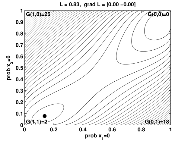
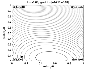
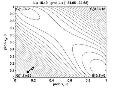
Figure 2: (a) Original Lagrangian function. The suboptimal local minimum is located at $q^{*}$ which is indicated with a dot in the lower left corner. (b) The Lagrangian under the coordinate transformation which minimizes $L(q^{*})$. (c) The Lagrangian under the coordinate transformation which maximizes the norm of the gradient at $q^{*}$. The direction of the negative gradient is indicated by a black arrow.

There are a number of criteria that might be used to determine a semicoordinate transformation to escape from this local minimum $q^{*}$. Two simple choices are to select the transformation that minimizes the new value of the maxent Lagrangian (i.e., minimize $L(q^{*})$), or to select the transformation which results in the largest gradient of the maxent Lagrangian at $q^{*}$, (i,e,, maximize $\|\nabla_{q}L(q^{*})\|$). For this simple problem the results of both these choices are shown as Figures 2(b) and 2(c) respectively. The transformation in each of these cases is determined by optimizing over semicoordinate transformations (permutations), while keeping the probabilities fixed, to either minimize the Lagrangian value at $q^{*}$, or maximize the norm of the gradient at $q^{*}$.

In principle, this semicoordinate search can be embedded within any optimization to dynamically escape local minima as they are encountered. Importantly, the search criteria listed above require no look ahead in order to identify the best semicoordinate permutation. However, in practice, since we can not search over arbitrarily large permutation spaces we must select a few of the variables and permute amongst their possible joint moves. By composing such permutations we can easily account for the escape from multiple local minima. Heuristics for the selection of “permuting” variables, and the results of this procedure await future work.

4.3 Semicoordinate Transformations for Mixture Distributions

In this section we turn to a different use of semicoordinate transformations. We have previously described how the Lagrangian measuring the distance of a product distribution to a Boltzmann distribution may be minimized in a distributed fashion. We now extend these results to mixtures of product distributions in order to represent multiple product distribution solutions at once. We can always do that by means of a semicoordinate transformation of the underlying variables. In this section we demonstrate this explicitly.

Let $\mathcal{X}$ indicate the set of variables in a space of dimension $d_{\mathcal{X}}$, and let $\mathcal{Z}$ be the original (pre-transformation) $n$-dimensional space over which $G$ is defined. We identify a product distribution over $\mathcal{X}$ (with $d_{\mathcal{X}}>n$), and an appropriately chosen mapping $\boldsymbol{\zeta}:\mathcal{X}\rightarrow\mathcal{Z}$ which induce a mixture distribution over $\mathcal{Z}$.

To see this consider an $M$ component mixture distribution over $n$ variables, which we write as: $q(z)=\sum_{m=1}^{M}q^{0}(m)q^{m}(\mathbf{z})$ with $\sum_{m=1}^{M}q^{0}(m)=1$ and $q^{m}(\mathbf{z})=\prod_{i=1}^{n}q^{m}_{i}(z_{i})$. We express this $q(\mathbf{z})$ as (the image of) a product distribution over a space $\mathcal{X}$ of dimension $d_{\mathcal{X}}=1+Mn$. Intuitively, the first dimension of $\mathcal{X}$ (indicated as $x^{0}\in[1,M]$) labels the mixture, and the remaining $Mn$ dimensions (indicated as $x^{m}_{i}\in\mathcal{Z}_{i}$) correspond to each of the original $n$ dimensions for each of the $M$ mixtures.

More precisely, write out the $\mathcal{X}$-space product distribution as $q_{\mathcal{X}}(\mathbf{x})=q^{0}(x^{0})\prod_{m=1}^{M}q^{m}(\mathbf{x}^{m})$ with $q^{m}(\mathbf{x}^{m})=\prod_{i=1}^{n}q^{m}_{i}(x^{m}_{i})$ for $\mathbf{x}=[x^{0},\mathbf{x}^{1},\cdots,\mathbf{x}^{M}]$ and $\mathbf{x}^{m}=[x^{m}_{1},\cdots,x^{m}_{n}]$. The density in $\mathcal{X}$ and $\mathcal{Z}$ are related as usual by $q(\mathbf{z})=\sum_{\mathbf{x}}q_{\mathcal{X}}(\mathbf{x})\delta\bigl{(}\mathbf{z}-\zeta(\mathbf{x})\bigr{)}$ with the delta function acting on vectors being understood component-wise. If we label the components of $\zeta$ so that $z_{i}=\zeta_{i}(x^{0},\mathbf{x}^{1},\cdots,\mathbf{x}^{M})\triangleq x_{i}^{x^{0}}$ we find

$$q(\mathbf{z}) =\sum_{x^{0}}q^{0}(x^{0})\sum_{\mathbf{x}^{1},\cdots,\mathbf{x}^{M}}\prod_{m}q^{m}(\mathbf{x}^{m})\prod_{i}\delta\bigl{(}z_{i}-\zeta_{i}(x^{0},\mathbf{x}^{1},\cdots,\mathbf{x}^{M})\bigr{)}$$

$$=\sum_{x^{0}}q^{0}(x^{0})\sum_{\mathbf{x}^{1},\cdots,\mathbf{x}^{M}}\prod_{m}q^{m}(\mathbf{x}^{m})\prod_{i}\delta\bigl{(}z_{i}-x^{x^{0}}_{i}\bigr{)}$$

$$=\sum_{x^{0}}q^{0}(x^{0})\sum_{\mathbf{x}^{x^{0}}}q^{x^{0}}(\mathbf{x}^{x^{0}})\prod_{i}\delta\bigl{(}z_{i}-x^{x^{0}}_{i}\bigr{)}$$

$$=\sum_{x^{0}}q^{0}(x^{0})q^{x^{0}}(\mathbf{z})$$

Thus, under $\zeta$ the product distribution $q_{\mathcal{X}}$ is mapped to the mixture of products $q(\mathbf{z})=\sum_{m}q^{0}(m)q^{m}(\mathbf{z})$ (after relabelling $x^{0}$ to $m$), as desired.

The maxent Lagrangian of the $\mathcal{X}$ product distribution $q_{\mathcal{X}}(\mathbf{x})$ is

$$\mathcal{L}_{\mathcal{X}}(q_{\mathcal{X}})=\sum_{m}q^{0}(m)\mathbb{E}_{q^{m}}(G)-T\Bigl{[}S(q^{0})+\sum_{m=1}^{M}S(q^{m})\Bigr{]}.$$

This Lagrangian contains a term pushing us (as we search for the minimizer of that Lagrangian) to maximize the entropy of the mixture weights, but it provides no incentive for the distributions $q^{m}$ to differ from each other. As we have argued, it is desirable to have the different mixtures capture different solutions, and so we modify the Lagrangian function slightly.

If we wish the $q^{m}$ differ from one another, we instead consider the maxent Lagrangian defined over $q(\mathbf{z})$. In this case

$$\mathcal{L}_{\mathcal{Z}}(q) =\sum_{\mathbf{z}}G\bigl{(}\mathbf{z})q(\mathbf{z})-TS(q)=\sum_{\mathbf{x}}G\bigl{(}\boldsymbol{\zeta}(\mathbf{x})\bigr{)}q_{\mathcal{X}}(\mathbf{x})-TS(q)$$

$$=\sum_{m}q^{0}(m)\mathbb{E}_{q^{m}}(G)-TS\biggl{(}\sum_{m}q^{0}(m)q^{m}(\mathbf{z})\biggr{)}.$$

The entropy term differs crucially in these two maxent Lagrangians. To see this add and subtract $T\sum_{m}q^{0}(m)S(q^{m})$ to the $\mathcal{Z}$ Lagrangian to find

$$\mathcal{L}_{\mathcal{Z}}(q)=\sum_{m}q^{0}(m)\mathcal{L}(q^{m})-TJ(q)$$ (14)

where each $\mathcal{L}(q^{m})$ is a maxent Lagrangian as given by Eq. (1), and $J(q)\geq 0$ is a modified version of the Jensen-Shannon (JS) distance,

$$J(q)=S\Bigl{(}\sum_{m}q^{0}(m)q^{m}\Bigr{)}-\sum_{m}q^{0}(m)S(q^{m})=-\sum_{m}\sum_{\mathbf{z}}q^{0}(m)q^{m}(\mathbf{z})\ln\frac{q(\mathbf{z})}{q^{m}(\mathbf{z})}.$$

Conventional Jensen-Shannon distance is defined to compare two distributions to each other, and gives those distributions equal weight. In contrast, the generalized JS distance $J(q)$ concerns multiple distributions, and weights them nonuniformly, according to $q^{0}(m)$.

$J(q)$ is maximized when the $q^{m}$ are all different from each other. Thus, its inclusion into the Lagrangian pushes the mixing components away (in $\mathcal{X}$) from one another. In this, we can view Eq. (14) as a novel derivation of (a generalized version of) Jensen-Shannon distance. Unfortunately, the JS distance also couples all of the variables (because of the sum inside the logarithm) which prevents a highly distributed solution.

To address this, in this paper we replace $J(q)$ in $\mathcal{L}_{\mathcal{Z}}(q)$ with another function which lower-bounds $J(q)$ but which requires less communication between agents. It is this modified Lagrangian that we will minimize.

4.4 A Variational Lagrangian

Following [jj98], we introduce $M$ variational functions $w(\mathbf{z}|m)$ and lower-bound the true JS distance. We begin with the identity

$$J(q) =-\sum_{m}\sum_{\mathbf{z}}q^{0}(m)q^{m}(\mathbf{z})\ln\left[\frac{1}{w(\mathbf{z}|m)}q^{0}(m)\frac{w(\mathbf{z}|m)q(\mathbf{z})}{q^{0}(m)q^{m}(\mathbf{z})}\right]$$

$$=\sum_{m}\sum_{\mathbf{z}}q^{0}(m)q^{m}(\mathbf{z})\ln w(\mathbf{z}|m))-\sum_{m}q^{0}(m)\ln q^{0}(m)$$

$$\phantom{=}-\sum_{m}\sum_{\mathbf{z}}q^{0}(m)q^{m}(\mathbf{z})\ln\frac{w(\mathbf{z}|m)q(\mathbf{z})}{q^{0}(m)q^{m}(\mathbf{z})}.$$

Now replace $M$ of the $-\ln$ terms with the lower bound $-\ln z\geq-\nu z+\ln\nu+1$ obtained from the Legendre dual of the logarithm to find

$$J(q)\geq J(q,w,\nu) \triangleq\sum_{m}\sum_{\mathbf{z}}q^{0}(m)q^{m}(z)\ln w(\mathbf{z}|m)-\sum_{m}q^{0}(m)\ln q^{0}(m)$$

$$\phantom{\geq}-\sum_{m}\nu_{m}\sum_{\mathbf{z}}w(\mathbf{z}|m)q(z)+\sum_{m}q^{0}(m)\ln\nu_{m}+1.$$

Optimization over $w$ and $\nu$ maximizes this lower bound. To further aid in distributing the algorithm we restrict the class of variational $w(\mathbf{z}|m)$ to products: $w(\mathbf{z}|m)=\prod_{i}w_{i}(z_{i}|m)$. For this choice

$$J(q,w,\nu) \triangleq\sum_{m}q^{0}(m)\left\{B^{m,m}-\sum_{\tilde{m}}A^{m,\tilde{m}}\nu_{\tilde{m}}+\ln\nu_{m}\right\}+S(q^{0})+1$$ (15)

where $A^{\tilde{m},m}_{i}\triangleq\sum_{z_{i}}q^{\tilde{m}}_{i}(z_{i})w_{i}(z_{i}|m)$, $A^{\tilde{m},m}\triangleq\prod_{i=1}^{d}A^{\tilde{m},m}_{i}$, $B^{m,m}_{i}\triangleq\sum_{z_{i}}q^{m}_{i}(z_{i})\ln w_{i}(z_{i}|m)$, and $B^{m,m}\triangleq\sum_{i=1}^{d}B^{m,m}_{i}$. At any temperature $T$ the variational Lagrangian which must be minimized with respect to $q$, $w$ and $\nu$ (subject to appropriate positivity and normalization constraints) is then

$$\mathcal{L}_{\mathcal{Z}}(q,w,\nu)=\sum_{m}q^{0}(m)\mathcal{L}(q^{m})-TJ(q,w,\nu)$$ (16)

with $J(q,w,\nu)$ given by Eq. (15).

5 Minimizing the Mixture Distribution Lagrangian

Equating the gradients with respect to $w$ and $\nu$ to zero gives

$$\frac{1}{\nu_{m}}=\frac{1}{q^{0}(m)}\sum_{\tilde{m}}q^{0}(\tilde{m})A^{\tilde{m},m}.$$ (17)

$$w_{i}(z_{i}|m)\propto\frac{q^{0}(m)q^{m}_{i}(z_{i})}{\nu_{m}}\left[\sum_{\tilde{m}}q^{0}(\tilde{m})q^{\tilde{m}}_{i}(z_{i})\frac{A^{\tilde{m},m}}{A^{\tilde{m},m}_{i}}\right]^{-1}.$$ (18)

The dependence of $\mathcal{L}_{\mathcal{Z}}$ on $q^{0}(m)$ is particularly simple: $\mathcal{L}_{\mathcal{Z}}(q,w,\nu)\approx\sum_{m}q^{0}(m)\mathcal{E}(m)-T\bigl{(}S(q^{0})+1\bigr{)}$ up to $q^{0}$-independent terms where

$$\mathcal{E}(m)\triangleq\mathbb{E}_{q^{m}}(G)-T\left(S[q^{m}]+B^{m,m}-\sum_{\tilde{m}}A^{m,\tilde{m}}\nu_{\tilde{m}}+\ln\nu_{m}\right),$$

Thus, the mixture weights are Boltzmann distributed with energy function $\mathcal{E}(m)$:

$$q^{0}(m)=\frac{\exp\bigl{(}-\mathcal{E}(m)/T\bigr{)}}{\sum_{\tilde{m}}\exp\bigl{(}-\mathcal{E}(\tilde{m})/T\bigr{)}}.$$ (19)

The determination of $q^{m}_{i}(z_{i})$ is similar. The relevant terms in $\mathcal{L}_{\mathcal{Z}}$ involving $q^{m}_{i}(z_{i})$ are $\mathcal{L}_{\mathcal{Z}}\approx q^{0}(m)\sum_{z_{i}}\mathcal{E}_{m}(z_{i})q^{m}_{i}(z_{i})-TS(q^{m}_{i})$ where

$$\mathcal{E}_{m}(z_{i})=\mathbb{E}_{q^{m}_{-i}}(G|z_{i})-T\biggl{(}\ln w_{i}(z_{i}|m)-\sum_{\tilde{m}}\frac{A^{m,\tilde{m}}}{A^{m,\tilde{m}}_{i}}\nu_{\tilde{m}}w_{i}(z_{i}|\tilde{m})\biggr{)}.$$

As before, the conditional expectation $\mathbb{E}_{q^{m}_{-i}}(G|z_{i})$ is $\sum_{z_{-i}}G(z_{i},\mathbf{z}_{-i})q^{m}_{-i}(\mathbf{z}_{-i})$. The mixture probabilities are thus determined as

$$q^{m}_{i}(z_{i})=\frac{\exp\bigl{(}-\mathcal{E}_{m}(z_{i})/T\bigr{)}}{\sum_{z_{i}}\exp\bigl{(}-\mathcal{E}_{m}(z_{i})/T\bigr{)}}.$$ (20)

5.1 Agent Communication

As desired these results require minimal communication between agents. A supervisory agent, call this the 0-agent, is assigned to manage the determination of $q^{0}(m)$, and $(i,m)$-agents manage the determination of $q^{m}_{i}(z_{i})$. The $M$ $(i,m)$-agents for a fixed $i$ communicate their $w_{i}(z_{i}|m)$ to determine $A^{m,\tilde{m}}_{i}$. These results along with the $B^{m,m}_{i}$ from each $(i,m)$ agent are then forwarded to the 0-agent who forms $A^{m,\tilde{m}}$ and $B^{m,m}$ broadcasts this back to all $(i,m)$-agents. With these quantities and the local estimates for $\mathbb{E}_{q^{m}_{-i}}(G|z_{i})$, all $q_{i}^{m}$ can be updated independently.

6 Experiments

In this section we demonstrate our methods on some simple problems. These examples are illustrative only, and for further examples the reader is directed to [biwo04a, biwo04b, biwo04c, lewo04b, wole04] for related experiments.

We test the the mixture semicoordinate probability collective method on two different problems: a $k$-sat constraint satisfaction problem having multiple feasible solutions, and optimization of an unconstrained optimization of an $NK$ function.

6.1 k-sat

The $k$-sat problem is perhaps the best studied CSP [mepa02]. The goal is to assign $N$ binary variables (labelled $z_{i}$) true/valse values so that $C$ disjunctive clauses are satisfied. The $a$th clause involves $k$ variables labelled by $v_{a,j}\in[1,N]$ (for $j\in[1,k]$), and $k$ binary values associated with each $a$ and labelled by $\sigma_{a,j}$. The $a$th clause is satisfied iff $\bigvee_{j=1}^{k}[z_{v_{a,j}}=\sigma_{a,j}]$ so we define the $a$th constraint as

$$c_{a}(\mathbf{z})=\begin{cases}0&\text{if}\;\bigvee_{j=1}^{k}[z_{v_{a,j}}=\sigma_{a,j}]\\ 1&\text{otherwise}\end{cases}.$$

As the $a$th clause is violated only when all $z_{v_{a,j}}=\overline{\sigma}_{a,j}$ (with $\overline{\sigma}$ defined to be $\text{not}\,\sigma$), the Lagrangian over product distributions can be written as $\mathcal{L}(q)=\boldsymbol{\lambda}^{\top}\mathbf{c}(q)-TS(q)$ where $\mathbf{c}(q)$ is the $C$-vector of expected constraint violations, and $\boldsymbol{\lambda}$ is the $C$ vector of Lagrange multipliers. The $a$’th component of $\mathbf{c}(q)$ is the expected violation of the $a$th clause, and is given by $c_{a}({q})\triangleq\sum_{\mathbf{z}}c_{a}(\mathbf{z})q(\mathbf{z})=\prod_{j=1}^{k}q_{v_{a,j}}(\overline{\sigma}_{a,j})$. Note that no Monte Carlo estimates are required to evaluate this quantity. Further, the only communication required to evaluate $G$, and its conditional expectations is between agents appearing in the same clause. Typically, this communication network is sparse; for the $N=100$, $k=3$, $C=430$ variable problem we consider here each agent interacts with only $6$ other agents on average.

   

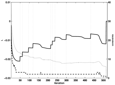
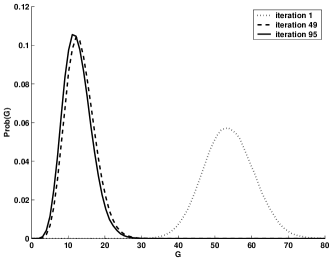
Figure 3: (a) Evolution of Lagrangian value (solid line), expected constraint violation (dotted line), and constraint violations of most likely configuration (dashed line). (b) ${P}(G)$ after minimizing the Lagrangian for the first 3 multiplier settings. At termination $P(G)=\delta(G)$.

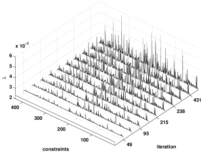
Figure 4: Each constraint’s Lagrange multiplier versus the iterations when they change.

We first present results for a single product distribution. For any fixed setting of the Lagrange multipliers, the Lagrangian is minimized by iterating Eq. (10). If the minimization is done by the Brouwer method, any random subset of variables, no two of which appear in the same clause, can be updated simultaneously. This eliminates “thrashing” and ensures that the Lagrangian decreases at each iteration.

The minimization is terminated at a local minimum ${q}^{*}$ which is detected when the norm of the gradient falls below a threshold. If all constraints are satisfied at ${q}^{*}$ we return the solution $\mathbf{z}^{*}=\operatornamewithlimits{arg\ max}_{\mathbf{z}}q^{*}(\mathbf{z})$, otherwise the Lagrange multipliers are updated according to Eq. (11). In the present context, this updating rule offers a number of benefits. Firstly, those constraints which are violated most strongly have their penalty increased the most, and consequently, the agents involved in those constraints are most likely to alter their state. Secondly, the Lagrange multipliers contain a history of the constraint violations (since we keep adding to $\boldsymbol{\lambda}$) so that when the agents coordinate on their next move they are unlikely to return a previously violated state. This mimics the approach used in taboo search where revisiting of configurations is explicitly prevented, and aids in an efficient exploration of the search space. Lastly, rescaling the Lagrangian after each update of the multipliers by $\boldsymbol{1}^{\top}\boldsymbol{\lambda}\triangleq\sum_{a}\lambda_{a}$ gives $\mathcal{L}({q})=\hat{\boldsymbol{\lambda}}{}^{\top}\mathbf{c}({q})-\hat{T}S({q})$ where $\hat{\boldsymbol{\lambda}}=\boldsymbol{\lambda}/\mathbf{1}^{\top}\boldsymbol{\lambda}$ and $\hat{T}=T/\mathbf{1}^{\top}\boldsymbol{\lambda}$. Since $\sum_{a}\hat{\lambda}_{a}=1$ the first term reweights clauses according to their expected violation, while the temperature $\hat{T}$ cools in an automated annealing schedule as the Lagrange multipliers increase. Cooling is most rapid when the expected constraint violation is large and slows as the optimum is approached. The parameters $\alpha_{\lambda}^{t}$ thus govern the overall rate of cooling. We used the fixed value $\alpha_{\lambda}^{t}=0.5$ in the reported experiments.

Figure 3 presents results for a 100 variable $k=3$ problem using a single mixture. The problem is satisfiable formula uf100-01.cnf from SATLIB (www.satlib.org). It was generated with the ratio of clauses to variables being near the phase transition, and consequently has few solutions. Fig. 3(a) shows the variation of the Lagrangian, the expected number of constraint violations, and the number of constraints violated in the most probable state ${z}_{\text{mp}}\triangleq\operatornamewithlimits{arg\ max}_{\mathbf{z}}q(\mathbf{z})$ as a function of the number of iterations. The starting state is the maximum entropy configuration of uniform $q_{i}$, and the starting temperature is $T=1.5\cdot 10^{-3}$. The iterations at which the Lagrange multipliers are updated are indicated by vertical dashed lines which are clearly visible as discontinuities in the Lagrangian values. To show the stochastic underpinnings of the algorithm we plot in Fig. 3(b) the probability density of the number of constraint violations obtained as $P(G)=\sum_{\mathbf{z}}q(\mathbf{z})\delta\bigl{(}G-\sum_{a}c_{a}(\mathbf{z})\bigr{)}$. We see the downward movement of the expected value of $G$ as the algorithm progresses. Figure 4 shows the evolution of the renormalized Langrange multipliers $\hat{\boldsymbol{\lambda}}$. At the first iteration the multiplier for all clauses are equal. As the algorithm progresses weight is shifted amongst difficult to satisfy clauses.

Results on a larger problem with multiple mixtures are shown in Fig. 5(a). This is the 250 variable/1065 clause problem uf250-01.cnf from SATLIB with the first 50 clauses removed so that the problem has multiple solutions. The optimization is performed by selecting a random subset of variables, no two of which appear in the same clause, at each iteration, and updating according to Eqs. (17), (18), (19), and (20). After convergence to a local minimum the Lagrange multipliers are updated as above according to the expected constraint violation. The initial temperature is $10^{-1}$. We plot the number of constraints violated in the most probable state of each mixture as a function of the number of updates. as well as the expected number of violated constraints. After 8000 steps three distinct solutions are found along with a fourth configuration which violates a single constraint.

  

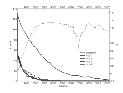
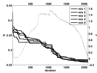
Figure 5: (a) The solid curves show the number of unsatisfied clauses in the most probable configuration $z_{\text{mp}}$ of each of the 4 mixtures vs iterations. The topmost solid black line plots the expected number of violations, and the dashed black line shows the approximation to the JS distance. (b) The solid curves show the evolution of the $G$ value of the best $z_{\text{mp}}$ configurations for each of 5 mixtures versus number of iterations. The dashed black line shows the corresponding approximation to the JS distance.

6.2 Minimization of NK Functions

Next we consider an unconstrained discrete optimization problem. The $NK$ model defines a family of tunably difficult optimization problems [KLNK]. The objective over $N$ binary variables $\{z_{i}\}_{i=1}^{N}$ is defined as the average of $N$ randomly generated contributions depending on $z_{i}$ and $K$ other randomly chosen variables $z_{i}^{1}\cdots z_{i}^{K}$: $G(\mathbf{z})=N^{-1}\sum_{i=1}^{N}E_{i}(z_{i};z_{i}^{1},\cdots z_{i}^{K})$. For each of the $2^{K+1}$ local configurations $E_{i}$ is assigned a value drawn uniformly from 0 to 1. $K$ which ranges between 0 and $N-1$ controls the number of local minima; under Hamming neighborhoods $K=0$ optimization landscapes have a single global optimum and $K=N-1$ landscapes have on average $2^{N}/(N+1)$ local minima. Further properties of $NK$ landscapes may be found in [durrett.limic.ea:rigorous]. Fig. 5(b) plots the energy of a 5 mixture model for a multi-modal $N=300$ $K=2$ function. The $K-1$ spins other than $i$ upon which $E_{i}$ depends were selected at random. At termination of the PC algorithm (at a small but non-zero temperature), five distinct configurations are obtained with the nearest pair of solutions having Hamming distance 12. Note that unlike the $k$-sat problem which has multiple configurations all having the same global minimal energy, the JS distance (the dashed curve) of Fig. 5(b) drops to zero as the temperature decreases. This is because at exactly zero temperature there is no term forcing different solutions, and the Lagrangian is minimized by having all mixtures converge to delta functions at the lowest objective value configuration. The effect of mixtures enables the algorithm to simultaneously explore multiple local extema before converging on the lowest objective solution.

7 Relation of PC to other work

There has been much work from many fields related to PC. The maxent Lagrangian has been used in statistical physics for over a century under the rubric of “free energy”. Its derivation in terms of information theoretic statistical inference was by Jaynes [jayn57]. The maxent Lagrangian has also appeared occasionally in game theory as a heuristic, without a statistical inference justification (be it information-theoretic or otherwise) [fule98, shar04]. In none of this earlier work is there an appreciation for its relationship with the related work in other fields.

In the context of distributed control/optimization, the distinguishing feature of PC is that it does not view the variable ${\mathbf{x}}$ as the fundamental object, but rather the distribution across it, $q$. Samples of that distribution are not the direct object of interest, and in fact are only used if necessary to estimate functionals of $q$. The fundamental objective function is stated in terms of $q$. As explicated in the next subsection, the associated optimization algorithms are related to some work in several fields. Heretofore those fields have been unaware of each other, and of the breadth of their relation to information theory and game theory.

Finally, we note that the maxent or $qp$ Lagrangian $\mathcal{L}(q)=E_{q}(G)-TS(q)$ can be viewed as a barrier-function (interior point) method with objective $E_{q}(G)$. An entropic barrier function is used to enforce the constraints $q_{i}(x_{i})\geq 0\;\forall i$ and $x_{i}$, with the constraint that all $q_{i}$ sum to 1 being implicit.

7.1 Various schemes for updating $q$

We have seen that the $qp$ Lagrangian is minimized by the product distribution $q$ given by

$$q_{i}(x_{i})\propto\exp\bigl{(}-E_{q_{-i}}(G|x_{i})/T\bigr{)}.$$ (21)

Direct application of these equations that minimize the Lagrangian form the basis of the Brouwer update rules. Alternatively, steepest descent of the maxent Lagrangian forms the basis of the Nearest Newton algorithm. These update rules have analogues in conventional (non-PC) optimization. For example, Nearest-Newton is based on Newton’s method, and Brouwer updating is similar to block-relaxation. This is one of the advantages of embedding the original optimization problem involving $x$ in a problem involving distributions across $x$: it allows us to solve problems over non-Euclidean (e.g., countable) spaces using the powerful methods already well-understood for optimization over Euclidean spaces.

However there are other PC update rules that have no direct analogue in such well-understood methods for Euclidean space optimization. Algorithms may be developed that minimize the $pq$ Lagrangian $D(p_{T}\|q)$ where $p_{T}(\mathbf{x})=\exp\bigl{(}-G(\mathbf{x})/T\bigr{)}/Z(T)$ with $Z(T)$ being the normalization of the Boltzmann distribution. The $pq$ Lagrangian is minimized by the the product of the marginals of the Boltzmann distribution, i.e. $q_{i}(x_{i})=\int d\mathbf{x}_{-i}\;p_{T}(\mathbf{x})$. Another example of update rules without Euclidean analogues are the iterative focusing update rules described in [wolp04g]. Iterative focusing updates are intrinsically tied into the fact that we’re minimizing (the distribution setting) an expectation value.

A subset of update rules arising from $qp$ and $pq$ Lagrangians are described in [wolp04g]. In all cases, the updates may be written as multiplicative updating of $q$. The following is a list of the update ratios $r_{q,i}(x_{i})\equiv q^{t+1}_{i}(x_{i})/q^{t}_{i}(x_{i})$ of some of those rules.

In all of the rules in this list, $F_{G}$ is a probability distribution over $x$ that never increases between two $x$’s if $G$ does (e.g., a Boltzmann distribution in $G(x)$). In addition, const is a scalar that ensures the new distribution is properly normalized and $\alpha$ is a stepsize. Finally, “iterative focusing” is a technique that repeats the following process: It takes a distribution $\tilde{q}$ as input. It then produces as output a new distribution that is $\tilde{q}$ “focused” more tightly about $x$’s with good $G(x)$. That focused distribution becomes $\tilde{q}$ for the next iteration. See [wost06].

Gradient descent of $qp$ distance to ${F_{G}}$:

$$1-\alpha\Bigl{\{}\frac{{\mathbb{E}}_{q^{t}}(\ln F_{G}|x_{i})+\ln(q^{t}_{i}(x_{i}))}{q^{t}_{i}(x_{i}\ )}\Bigr{\}}-\frac{\text{const}}{q^{t}_{i}(x_{i})}$$ (22)

Nearest Newton descent of $qp$ distance to ${F_{G}}$:

$$1-\alpha\bigl{\{}{\mathbb{E}}_{q^{t}}(\ln F_{G}|x_{i})+{\mbox{ln}}(q^{t}_{i}(x_{i}))\bigr{\}}-\text{const}$$ (23)

Brouwer updating for $qp$ distance to ${F_{G}}$:

$$\text{const}\times\frac{e^{{\mathbb{E}}_{q^{t}}(\ln F_{G}|x_{i})}}{q^{t}_{i}(x_{i})}$$ (24)

Importance sampling minimization of $pq$ distance to $F_{G}$:

$$\text{const}\times{\mathbb{E}}_{q^{t}}\biggl{(}\frac{F_{G}}{q^{t}}|x_{i}\biggr{)}$$ (25)

Iterative focusing of ${\tilde{q}}$ with focusing function ${F_{G}}$ using $qp$ distance and gradient descent:

$$1-\alpha\Bigl{\{}\frac{{\mathbb{E}}_{q^{t}}(\ln F_{G}|x_{i})+\ln\frac{q^{t}_{i}(x_{i})}{{\tilde{q}}_{i}(x_{i})}}{q^{t}(x_{i})}\Bigr{\}}-\frac{\text{const}}{q^{t}(x_{i})}$$ (26)

Iterative focusing of ${\tilde{q}}$ with focusing function ${F_{G}}$ using $qp$ distance and Nearest Newton:

$$1-\alpha\Bigl{\{}{\mathbb{E}}_{q^{t}}(\ln F_{G}|x_{i})+\ln\frac{q^{t}_{i}(x_{i})}{{\tilde{q}}_{i}(x_{i})}\Bigr{\}}-\text{const}$$ (27)

Iterative focusing of ${\tilde{q}}$ with focusing function ${F_{G}}$ using $qp$ distance and Brouwer updating:

$$\text{const}\times e^{{\mathbb{E}}_{q^{t}}(\ln F_{G}|x_{i})}\times\frac{{\tilde{q}}(x_{i})}{q_{i}^{t}(x_{i})}$$ (28)

Iterative focusing of ${\tilde{q}}$ with focusing function $F_{G}$ using $pq$ distance:

$$\text{const}\times{\mathbb{E}}_{\tilde{q}}(F_{G}|x_{i})\times\frac{\tilde{q}(x_{i})}{q_{i}^{t}(x_{i})}$$ (29)

Note that some of these update ratios are themselves proper probability distributions, e.g., the Nearest Newton update ratio.

This list highlights the ability to go beyond conventional Euclidean optimization update rules, and is an advantage of embedding the original optimization problem in a problem over a space of probability distributions. Another advantage is the fact that the distribution itself provides much useful information (e.g., sensitivity information). Yet another advantage is the natural use of Monte Carlo techniques that arise with the embedding, and allow the optimization to be used for adaptive control.

7.1.1 Relation of PC to other distribution-based optimization algorithms

There is some work on optimization that precedes PC and that has directly considered the distribution $q$ as the object of interest. Much of this work can be viewed as special cases of PC. In particular deterministic annealing  [duha00] is “bare-bones” parallel Brouwer updating. This involves no data-aging (or any other scheme to avoid thrashing of the agents), difference utilities, etc..

More tantalizingly, the technique of probability matching [sajo] uses Monte Carlo sampling to optimize a functional of $q$. This work was in the context of a single agent, and did not exploit techniques like data-ageing. Unfortunately, this work was not pursued.

Other work has both viewed $q$ as the fundamental object of interest and used techniques like data-aging and difference utilities. In particular, this is the case with the COllective INtelligence (COIN) work [wotu99a, wotu03a, wolp02]. However this work was not based on information-theoretic considerations and had no explicit objective function for $q$. It was the introduction of such considerations that resulted in PC.

Another interesting body of early work is the cross entryop (CE) method [rukr04]. This work is the same as iterative focusing using $pq$ distance. The CE method does not consider the formal difficulty with iterative focusing identified in [wost06], or any of the potential solutions to that problem discussed there. That difficulty means that even with no sampling error (i.e., if all estimated quantities are in fact exactly correct), in general there are no guarantees that the algorithm converges to an optimal $x$.

Other early work grew out of the Genetic Algorithms community. This work was initiated with MIMIC [deis97], and has since developed into the Estimation of Distribution Algorithms (EDA) approach [lola05]. A number of important issues were raised in this early work, e.g., the importance of information theoretic concepts.

For the most part however, especially in its early stages (e.g., with MIMIC), this work viewed the samples as the fundamental object of interest, rather than view the distribution being sampled that way. Little concern arises for what the objective function of the distribution being sampled should be, and of how samples can be used to achieve that optimization.

This means that there is little concern for issues like the (lack of) convexity of that implicit objective function. This prevents EDA’s from fully exploiting the power of continuous space optimization, e.g., the absence of local minima with convex problems [bova03]. Similarly, it means that with EDA’s there is no concern for cases where the distribution objective function can be optimized in closed form, without any need for sampling at all. Nor is there widespread appreciation for how old sample $x$’s can be re-used to help guide the optimization (as for example they are in PC’s adaptive importance sampling [wost06]).

This contrasts with PC, whose distinguishing feature is that it does not treat the variable ${\mathbf{x}}$ as the fundamental object to be optimized, but rather the distribution across it, $q$. So for example, in PC, samples of that distribution are only used if necessary to estimate quantities that cannot be evaluated other ways; the fundamental objective function is stated in terms of $q$. Indeed, in the cases considered in this paper, as well as earlier PC work like that reported in [mawo04a], no such samples of $q$ arise.

Shortly after the introduction of PC, a variant of its Monte Carlo version of parallel Brouwer updating has been introduced, called the MCE method [rubi05]. In this variant the annealing of the Lagrangian doesn’t involve changing the temperature $\beta$, but instead changing the value of a constraint specifying $\mathbb{E}_{q}(G)$. Accordingly, rather than jump directly to the ($\beta$-specified) solution given above, one has to solve a set of coupled nonlinear equations relating all the $q_{i}$. (Another distinguishing feature is no data-ageing, difference utilities or the like are used in the MCE method.) The MCE method has been justified with the KL argument reviewed above rather than with “ratchet”-based maximum entropy arguments. This has redrawn attention to the role of the argument-ordering of the KL distance, and how it relates Brouwer updating and the CE method.

Another body of work related to PC is (loopy) propagation algorithms, Bethe approximations, and the like  [mack03]. These techniques can be seen as an alternative to semicoordinate transformations for how to go beyond product distributions. Unlike those approaches, we are guaranteed to reach a local minimum of free energy. (If we were to use $pq$ KL distance rather than $qp$ KL distance, we would get to a $global$ minimum of free energy.) In addition, via utilities like AU and WLU (see appendix), we can exploit variance reduction techniques absent from those other techniques. Similarly those other techniques do not make use of data-aging.

Finally, there is also work that has been done after the introduction of both the CE method and PC that is closely related to both. Such methods are typically sample based, and a good summary of these approaches can be found in [muho05]. The use of junction tree factorizations for $q$ utilized in the above methods can be extended to PC theory, and results along these lines will be presented elsewhere.

8 Conclusion

A distributed constrained optimization framework based on probability collectives has been presented. Motivation for the framework was drawn from an extension of full-rationality game theory to bounded rational agents. An algorithm that is capable of obtaining one or more solutions simultaneously was developed and demonstrated on two problems. The results show a promising, highly distributed, off-the-shelf approach to constrained optimization.

There are many avenues for future exploration. Alternatives to the Lagrange multiplier method used here can be developed for constraint satisfaction problems. By viewing the constraints as separate objectives, a Pareto-like optimization procedure may be developed whereby a gradient direction is chosen which is constrained so that no constraints are worsened. This idea is motivated by the highly successful WalkSAT [skc93] algorithm for $k$-sat in which spins are flipped only if no previously satisfied clause becomes unsatisfied as a result of the change.

Probability collectives also offer promise in devising new methods for escaping local minima. Unlike traditional optimization methods where monotonic transformations of the objective leave local minima unchanged, such transformations will alter the local minima structure of the Lagrangian. This observation, and alternative Lagrangians (see [Rub01] for a related approach using a different minimization criterion) offer new approaches for improved optimization.

ACKNOWLEDGEMENTS We would like to thank Charlie Strauss for illuminating conversation and Bill Dunbar and George Judge for helpful comments on the manuscript.

Notes

1. 1 $|\mathcal{S}|$ denotes the number of elements in the set $\mathcal{S}$.
2. 2 In this paper vectors are indicated in bold font and scalars are in regular font.
3. 3 Despite its popularity, the KL distance $D(q\|p)$ between two probability distributions $q$ and $p$ is not a proper metric. It is not even symmetric between $q$ and $p$. However it is non-negative, and equals zero only when $q=p$.
4. 4 Here and throughout, we fix the convention that it is desirable to minimize objective functions, not to maximize them.
5. 5 We adopt the notation that $q_{-i}$ indicates the distribution $q$ with variable $i$ marginalized out, i.e., the product $\prod_{j\neq i}q_{j}$. Analogously, $\mathbf{x}_{-i}\triangleq[x_{1},\cdots,x_{i-1},x_{i+1},\cdots,x_{n}]$
6. 6 Properly speaking one should find the global minimizer $q$. Here we content ourselves with finding local minima.
7. 7 N.b., we do not project onto $\mathcal{Q}$ but rather add a vector to get back to it. See  [wobi04a].
8. 8 For such a distribution we relax the requirement of being a product or having any other particular form; we only require that all $0\leq\pi(\mathbf{x})\leq 1$ and $\sum_{\mathbf{x}}\pi(\mathbf{x})=1$.
9. 9 The Jacobian factor is irrelevant as $\zeta$ is a permutation.
10. 10 Alternatively, we can parameterize a smaller space of candidate permutations and select the best from amongst this candidate set.
11. 11 Note that if $w_{i}(z_{i}|m)=1/|\mathcal{Z}_{i}|$ is uniform across $z_{i}$ then $A^{\tilde{m},m}_{i}=1/|\mathcal{Z}_{i}|$ and $B^{m,m}_{i}=-\ln|\mathcal{Z}_{i}|$. Maximizing over $\nu_{m}$ we find that $J(q,w=1/|\mathcal{Z}|,\nu=\nu^{*})=0$. Thus, maximizing with respect to $w$ increases the JS distance from 0.
12. 12 In determining the density $10^{4}$ samples were drawn from $q(\mathbf{z})$ with Gaussians centered at each value of $G(\mathbf{z},{\bf{1}})$ and with the width of all Gaussians determined by cross validation of the log likelihood. The fact that there is non-zero probability of obtaining non-integral numbers of constraint violations is an artifact of the finite width of the Gaussians.
13. 13 However an attempt at a first-principles derivation can be found in [megi76].
14. 14 As a practical matter, both Nearest Newton and gradient-based updating have to be modified in a particular step if their step size is large enough so that they would otherwise take one off the unit simplex. This changes the update ratio for that step. See [wobi04a].
15. 15 Indeed, as conventionally cast, deterministic annealing assumes the conditional $G$ can be evaluated in closed form, and therefore has no concern for Monte Carlo sampling issues.
16. 16 Another alternative is to use data-ageing so that data from preceding Monte Carlo blocks can be re-used. Yet another alternative is to force a sample for each $x_{i}$ value that has no samples at the end of the block, $x^{\prime}_{i}$. This is done by drawing a random sample of the distribution $\delta(x_{i}-x^{\prime}_{i})q_{-i}(\mathbf{x}_{-i})$.
17. 17 To Monte Carlo estimate a conditional expected utility for agent $i$ it is crucial that $\mathbf{x}_{-i}$ be generated by sampling the associated distribution $q_{-i}$. However the value $x_{i}$ can be set in any fashion whatsoever.
18. 18 Just like AU, less sophisticated versions of WLU were previously explored under the same name, with examples again arising in  [wotu01a, wowh00] and references therein.
19. 19 To see this, say we add a function $D^{i}(\mathbf{x}_{-i})$ to $G({\mathbf{x}})$ both places $G$ occurs in the Nearest Newton update rule. Then since $q_{i}(x_{i})$ is evaluated exactly, the data average of the empirical estimates of those two terms involving $D^{i}$ both give the expectation value $\alpha^{t}q_{i}^{t}(x_{i}){\mathbb{E}}_{q^{t}_{-i}}(D^{i})$ exactly. Accordingly, those two terms cancel.
20. 20 Quadratic loss can be roughly related to the assumption that the Lagrangian is locally well-approximated by a paraboloid. We want to estimate $\mathbf{f}$ using an estimator $\hat{\mathbf{f}}(n)$ which is a function of prior information $n$. If we penalize errors quadratically (i.e. the error incurred when the estimate is $\hat{\mathbf{f}}$ and the true value is $\mathbf{f}$ is $\text{Err}(\mathbf{f},\hat{\mathbf{f}})=\|\hat{\mathbf{f}}-\mathbf{f}\|^{2}$), then the expected error conditioned on $n$ is $\mathbb{E}_{\mathbf{f}|n}(\text{Err})=\int d\mathbf{f}\,P(\mathbf{f}|n)\|\hat{\mathbf{f}}-\mathbf{f}\|^{2}=\|\hat{\mathbf{f}}\|^{2}-2\hat{\mathbf{f}}^{\top}\mathbb{E}_{\mathbf{f}|n}(\mathbf{f})+\mathbb{E}_{\mathbf{f}|n}(\|\mathbf{f}\|^{2})$. Minimizing this with respect to the estimator $\hat{\mathbf{f}}$ gives the optimal quadratic loss estimator $\hat{\mathbf{f}}(n)=\mathbb{E}_{\mathbf{f}|n}(\mathbf{f})$ Uncertainty in $\mathbf{f}$ arises due to uncertainty in $q_{-i}$, and hence we integrate over the unknown $q$.
21. 21 The bias-variance decomposition decomposes the error of an estimator into two contributions. Again let $f$ be the true quantity and let $\hat{f}(n)$ be an estimator of $f$ formed from data $n$. We are interested in the error $\text{Err}(\hat{f},f)=(\hat{f}-f)^{2}$ when averaged over different data sets $n$ so we consider $\mathbb{E}_{f,n}(\text{Err})=\int dndf\,P(n,f)(\hat{f}-f)^{2}$. By adding and subtracting $\mathbb{E}_{f}(f)-\mathbb{E}_{n}(\hat{f})$ we have $\mathbb{E}_{f,n}(\text{Err})=\int dndf\,P(n,f)\bigl{(}\{\hat{f}-\mathbb{E}_{n}(\hat{f})\}+\{\mathbb{E}_{f}(f)-f\}+\{\mathbb{E}_{n}(\hat{f})-\mathbb{E}_{f}(f)\}\bigr{)}^{2}$. The cross term vanish when integrating, and we are left with $\mathbb{E}_{f,n}(\text{Err})=\mathbb{E}_{n}\bigl{(}[\hat{f}-\mathbb{E}_{n}(\hat{f})]^{2}\bigr{)}+\mathbb{E}_{f}\bigl{(}[f-\mathbb{E}_{f}(f)]^{2}\bigr{)}+\bigl{[}\mathbb{E}_{f}(f)-\mathbb{E}_{n}(\hat{f})\bigr{]}^{2}$. The first term is the variance of the estimator across different data sets. The second term is the noise inherent in the quantity being estimated which is independent of the estimator, and which we will therefore ignore. The final term is the square of the bias of the estimator.

Appendix A Statistical estimation to update $q$

Using either of the update rules Eqs. (9) or (10) requires knowing $\mathbb{E}_{q^{t}_{-i}}\!(G|x_{i})$, defined in Eq. (7). However, often we cannot efficiently calculate all the terms $\mathbb{E}_{q^{t}_{-i}}\!(G|x_{i})$. To use our update rules in such situations we can use Monte Carlo sampling, as described in this section.

A.1 Monte Carlo sampling

In the Monte Carlo approach, at each timestep every agent $i$ samples its distribution $q_{i}$ to get a point $x_{i}$. Since we have a product distribution $q$, these samples provides us with a sample $\mathbf{x}$ of the full joint distribution $q$. By repeating this process $L$ times we get a “block” of such joint samples. The $G$ values in that block can be used by each agent separately to estimate its updating values $\mathbb{E}_{q^{t}_{-i}}\!(G|x_{i})$, for example simply by uniform averaging of the $G$ values in the samples associated with each $x_{i}$. Note that the single set of samples can be used no matter how many agents are in the system; we don’t need a different Monte Carlo process for each agent to estimate their separate $\mathbb{E}_{q^{t}_{-i}}\!(G|x_{i})$.

All agents (variables) sample moves (variable settings) independently, and coupling occurs only in the updates of the $q_{i}$. As we have seen this update (even to second order) for agent $i$ depends only on the conditional expectations $\mathbb{E}_{q_{-i}}(G|x_{i})$ where $q_{-i}$ describes the strategies used by the other agents. Thus, if we are using Monte Carlo, then the only information which needs to be communicated to each agent is the $G$ values upon which the estimate will be based. Using these values each agent independently updates its strategy (its $q_{i}$) in a way which collectively is guaranteed to lower the Lagrangian.

If the expectation is evaluated analytically, the $i$th agent needs the $q_{j}$ distributions for each of the $j$ agents involved in factors in $G$ that also involve $i$. For objective functions which consists of a sum of local interactions each of which individually involves only a small subset of the variables (e.g. the problems considered here), the number of agents that $i$ needs to communicate with is typically much smaller than $n$.

A.2 Difference utilities for faster Monte Carlo convergence

The basic Monte Carlo approach outlined above can be slow to converge in high-dimensional problems. For the problems considered in this paper this is irrelevant, since $\mathbb{E}_{q^{t}_{-i}}\!(G|x_{i})$ may be efficiently calculated in closed form for all agents $i$ and their moves $x_{i}$, so we don’t need to use Monte Carlo sampling. For completeness though here we present details of an improvement of the basic Monte Carlo approach that converges far more quickly.

Scrutiny of the two update rules (9) and (10) reveals that we don’t actually require the values $\mathbb{E}_{q^{t}_{-i}}\!(G|x_{i})$ for all $x_{i}$. All that is needed are the differences $\mathbb{E}_{q^{t}_{-i}}\!(G|x_{i})-\mathbb{E}_{q^{t}_{-i}}\!(G|x^{\prime}_{i})$ for pairs of distinct moves $x_{i}$ and $x^{\prime}_{i}$. (For both update rules the other degrees of freedom in the values $\mathbb{E}_{q^{t}_{-i}}\!(G|x_{i})$ are absorbed into the factor in the update rule ensuring normalization of $q_{i}$.) In other words, to update $q_{i}$ we can replace the sample averages of $G(\mathbf{x})$ with the sample averages of the associated difference utility $g^{i}(\mathbf{x})=G(\mathbf{x})-D^{i}(\mathbf{x}_{-i})$ for any function $D^{i}(\mathbf{x}_{-i})$. The differences in expectation values $\mathbb{E}_{q^{t}_{-i}}\!(g^{i}|x_{i})-\mathbb{E}_{q^{t}_{-i}}\!(g^{i}|x^{\prime}_{i})$ are invariant with respect to choice of $D^{i}$. However the choice of $D^{i}$ can have a major effect on the statistical accuracy of our Monte Carlo estimation.

We exploit the freedom granted by the introduction of $D^{i}(\mathbf{x}_{-i})$ to derive quantities which may be more easily estimated by Monte Carlo methods. In particular, we may define $D^{i}$ by requiring that the maximum likelihood estimator of the gradient has the lowest possible variance. In appendix B we show that the choice

$$D^{i}(\mathbf{x}_{-i})=\biggl{[}\sum_{x^{\prime\prime}_{i}}\frac{1}{L_{x^{\prime\prime}_{i}}}\biggr{]}^{-1}\sum_{x^{\prime}_{i}}\frac{G(x^{\prime}_{i},\mathbf{x}_{-i})}{L_{x^{\prime}_{i}}}.$$ (30)

gives the lowest possible variance. In the above equation $L_{x_{i}}$ is the numbers of times that the $i$th variable assumed value $x_{i}$ in a block of $L$ Monte Carlo samples.

The associated difference utility, $g^{i}(\mathbf{x})=G({\mathbf{x}})-D^{i}(\mathbf{x}_{-i})$, is called the Aristocrat utility (AU). An approximation to it was investigated in [wotu01a, wotu04, wotu02a] and references therein. AU itself was derived in  [wolp03a]. AU minimizes variance of gradient descent updating regardless of the form of $q$.

Sometimes not all the terms in the sum in AU can be stored, because $|\mathcal{X}_{i}|$ and/or the block size is too large. That sum can be approximated by replacing the $L_{x_{i}}$ values in the definition of AU with $q(x_{i})L$. This replacement also provides a way to address cases where one or more $L_{x_{i}}=0$. Similarly, for computational reasons it may be desirable to approximate the weighted average of $G$ over all $x^{\prime}_{i}$ which defines AU.

The sum over $x^{\prime}_{i}$ occurring in AU should not be confused with the sum over $x^{\prime}_{i}$ in Eq. (8) that pulls the gradient estimate back into the unit simplex. The sum here is over values of $G$ for counterfactual sample pairs $(x^{\prime}_{i},\mathbf{x}_{-i})$. (The other sum is over values of our gradient estimate at all of its arguments.) When the functional form of $G$ is known it is often the case that there is cancellation which allows AU be calculated directly, in one evaluation, an evaluation which can be cheaper than that of $G(\mathbf{x})$. When this is not the case their evaluation incurs a computational cost in general. This cost is offset by the fact that those evaluations allow us to determine the value of AU not just for the actual point $(x_{i},\mathbf{x}_{-i})$, but in fact for all points $\{(x_{i}^{\prime},\mathbf{x}_{-i})|x^{\prime}_{i}\in\mathcal{X}_{i}\}$.

Nonetheless, there will be cases where evaluating AU requires evaluating all possible $G(x^{\prime}_{i},\mathbf{x}_{-i})$, and where the cost of that is prohibitive, even if it allows us to update AU for all $x_{i}$ at once. Fortunately there are difference utilities that are cheaper to evaluate than AU while still having less variance than $G$. In particular, note that the weighting factor $L_{x^{\prime}_{i}}^{-1}/\sum_{x^{\prime\prime}_{i}}L_{x^{\prime\prime}_{i}}^{-1}$ in the formula for AU is largest for those $x_{i}$ which occur infrequently, i.e. that have low $q_{i}(x_{i})$. This observation leads to the Wonderful Life Utility (WLU), which is an approximation to AU that (being a difference utility) also has zero bias:

$$\mbox{$g^{WLU}_{i}(x_{i},\mathbf{x}_{-i})=G(x_{i},\mathbf{x}_{-i)})-G(x^{\text{clamp}}_{i},\mathbf{x}_{-i})$}.$$ (31)

In this formula, $x^{\text{clamp}}_{i}=\operatornamewithlimits{arg\ min}_{x_{i}}L_{x_{i}}$ or if we wish to be more conservative, $\operatornamewithlimits{arg\ min}_{x_{i}}q_{i}(x_{i})$, agent $i$’s lowest probability move [wolp03b, wolp04a].

Given the derivation of AU, one would expect that in general WLU will work best if $x^{\text{clamp}}_{i}$ is set to the $x$ that is least likely. As the run unfolds, which $x$ has that property will change. However changing $x^{\text{clamp}}_{i}$ accordingly will void the assumptions underlying the derivation of AU. In practice then, while one usually can update $x^{\text{clamp}}_{i}$ in such a dynamic fashion occasionally, doing so too frequently can cause problems.

A.3 Discussion of Monte Carlo sampling

Note that the foregoing analysis breaks down if any of the $L_{x_{i}}=0$. More generally it may break down if just one or more of the $q(x_{i})$ are particularly small in comparison to the others, even if no $L_{x_{i}}$ is exactly zero. The reason for this is that our approximation of the average over $n_{i}^{x}$ (see Appendix B) with the average where no $L_{x_{i}}=0$ breaks down. Doing the exact calculation with no such approximation doesn’t fix the situation — once we have to assign non-infinitesimal probability to $L_{x_{i}}=0$, we’re allowing a situation in which the gradient step would take us off the simplex of allowed $q\in\cal{Q}$. We might try to compensate for this by reducing the stepsize, but in general the foregoing analysis doesn’t hold if stepsize is reduced in some situations but not in any others. (Variable stepsize constitutes a change to the update rule. Such a modification to the update rule must be incorporated into the analysis — which obviates the derivation of AU.)

One way to address this scenario would be to simply zero out the probability of agent $i$ making any move $x_{i}$ for which $q_{i}(x_{i})$ is particular small. In other words, we can redefine $i$’s move space to exclude any moves if their probability ever gets sufficiently small. This has the additional advantage of reducing the amount of “noise” that agents $j\neq i$ will see in the next Monte Carlo block, since the effect of agent $i$ on the value of $G$ in that block is more tightly constrained.

There several ways to extend the derivation of AU, which only addresses estimation error for a single agent at a time, and for just that agent’s current update. One such extension is to have agent $i$’s utility set to improve the accuracy of the update estimation for agents $j\neq i$. For example, we could try to bias $q_{i}$ to be peaked about only a few moves, thereby reducing the amount of noise those other agents $j\neq i$ will see in the next Monte Carlo block due to variability in $i$’s move choice. Another extension is to have agent $i$’s utility set to improve the accuracy of its estimate of its update for future Monte Carlo blocks, even at the expense of accuracy for the current block.

Strictly speaking, the derivation of AU only applies to gradient descent updating of $q$. Difference utilities are unbiased estimators for the Nearest Newton update rule, so long as each $i$ estimates $\mathbb{E}_{q^{t}}(g^{i})$ as $q^{t}_{i}(x_{i})$ times the estimate of $\mathbb{E}_{q^{t}}(g^{i}|x_{i})$,

$$\sum_{x_{i}}{\hat{g}}^{i}_{x_{i}}(n_{i})q^{t}_{i}(x_{i})$$

rather than as the empirical average over all samples of $g^{i}$,

$$\sum_{x_{i}}{\hat{g}}^{i}_{x_{i}}(n_{i})\frac{L_{x_{i}}}{L}.$$

However the calculation for how to minimize the variance must be modified. Redoing the algebra above, the analog of AU for the Nearest Newton rule arises if we replace

$$\frac{1}{L_{x_{i}}}\rightarrow\frac{[q_{i}(x_{i})]^{2}}{L_{x_{i}}}\biggl{\{}[1-q_{i}(x_{i})]^{2}+\sum_{x^{\prime}_{i}\neq x_{i}}[q_{i}(x^{\prime}_{i})]^{2}\biggr{\}}$$ (32)

throughout the equation defining AU. Similar considerations apply to Brouwer updating as well. Nonetheless, in practice AU and WLU as defined above work well (and in particular far better than taking $g^{i}=G$) for the other updating rules as well.

For gradient descent updating, minimizing expected quadratic error of our estimator of $\mathbb{E}_{q^{t}_{-i}}\!(G|x_{i})$ corresponds to making a quadratic approximation to the Lagrangian surface, and then minimizing the expected value of the Lagrangian after the gradient step [wolp03b]. More generally, and especially for other update rules, some other kind of error measure might be preferable. Such measures would differ from the bias-variance decomposition. We do not consider such alternatives here.

Note that the agents are completely “blind” in the Monte Carlo process outline above, getting no information from other agents other than the values of $G({\mathbf{x}})$. When we allow some information to be transmitted between the agents we can improve the estimation of $\mathbb{E}_{q^{t}_{-i}}\!(G|x_{i})$ beyond that of the simple Monte Carlo process outlined above. For example, say that at every timestep the agent $i$ knows not just its own move $x_{i}$, but in fact the joint move ${\mathbf{x}}$. Then as time goes on it accumulates a training set of pairs {$({\mathbf{x}},G({\mathbf{x}}))$}. These can be used with conventional supervised learning algorithms [duha00] to form a rough estimate, ${\hat{G}}$, of the entire function $G$. Say that in addition $i$ knows not its own distribution $q_{i}(x^{t}_{i})$, but in fact the entire joint distribution, $q({\mathbf{x}}^{t})$. Then it can use that joint distribution together with ${\hat{G}}$ to form an estimate of $\mathbb{E}_{q^{t}_{-i}}\!(G|x_{i})$. That estimate is in addition to the one formed by the blind Monte Carlo process outlined above. One can then combine these estimates to form one superior to both. See [lewo04b].

Even when we are restricted to a blind Monte Carlo process, there are many heuristics that when incorporated into the update rules that can greatly improve their performance on real-world problems. In this paper we examine problems for which joint distributions $q$ are known to all agents as well as the function form of $G({\mathbf{x}})$ and the required expectations $\mathbb{E}_{q^{t}_{-i}}\!(G|x_{i})$ may be obtained in closed form. So there is no need for Monte Carlo approximations. Accordingly there is no need for those heuristics, and there is not even any need to using difference utilities. Empirical investigations of the effects of using difference utility functions and the heuristics may be found in  [biwo04a, biwo04b, biwo04c].

Appendix B Utility Derivation

Say we are at a timestep $t$ at the end of a Monte Carlo block, and consider the simplest updating rule. This is gradient descent updating, in which we wish to update $q_{i}$ at a timestep $t$ by having each agent $i$ take a small step in the direction (cf. Eq. (5))

$$\mathbf{f}^{i,G}\triangleq-\biggl{[}\frac{\partial\mathcal{L}(q^{t})}{\partial q_{i}(x_{i}^{1})},\cdots,\frac{\partial\mathcal{L}(q^{t})}{\partial q_{i}(x_{i}^{|\mathcal{X}_{i}|})}\biggr{]}-\eta_{i}(q)\mathbf{1}$$

where $\eta_{i}(q)$ was defined in Eq. (8), $\mathbf{1}$ is the vector of length $|\mathcal{X}_{i}|$ all of whose components are 1, and $x_{i}^{1},\cdots,x_{i}^{|\mathcal{X}_{i}|}$ are the $|\mathcal{X}_{i}|$ moves available to agent $i$. In general, there will be some error in $i$’s estimate of that step, since it has limited information about $q_{-i}^{t}$. Presuming quadratic loss reflects quality of the update, for agent $i$ the Bayes-optimal estimate of its update is the posterior expectation

$$\int dq^{t}\;P(q_{-i}^{t}\mid n_{i})\,\mathbf{f}^{i,G}$$

where $n_{i}$ is all the prior knowledge and data that $i$ has, and the dependence of $\mathbf{f}^{i,G}$ on $q_{-i}^{t}$ is implicit. $P(q_{-i}^{t}|n_{i})$ is a probability distribution over likely values of $q_{-i}^{t}$ given the information $n_{i}$ available to agent $i$.

Now agent $i$ can evaluate $\ln q_{i}(x_{i})$ for each of its moves $x_{i}$ exactly. However to perform its update it still needs the integrals

$$\int dq^{t}\;P(q_{-i}^{t}|n_{i})\,\mathbb{E}_{q^{t}_{-i}}\!(G|x_{i})$$

(recall Eq. (6)). In general these integrals can be very difficult to evaluate. As an alternative, we can replace those integrals with simple maximum likelihood estimators of them, i.e., we can use Monte Carlo sampling. In this case, the prior information, $n_{i}$, available to the agent is a list, $\mathfrak{L}$, of $L$ joint configurations $\mathbf{x}$ along with their accompanying objective values $G(\mathbf{x})$.

To define this precisely, for any function $h(\mathbf{x})$, let $\hat{\mathbf{h}}(n_{i})$ be a vector of length $|\mathcal{X}_{i}|$ which is indexed by $x_{i}$. The $x_{i}$ component of $\hat{\mathbf{h}}(n_{i})$ is indicated as $\hat{h}_{x_{i}}(n_{i})$. Each of its components is given by the information in $n_{i}$. The $x_{i}$’th such component is the empirical average of the values that $h$ had in the $L_{x_{i}}$ samples from the just-completed Monte Carlo block when agent $i$ made move $x_{i}$, i.e.

$$\hat{h}_{x_{i}}(n_{i})=\frac{1}{L_{x_{i}}}\sum_{\mathbf{x}\in\mathfrak{L}_{x_{i}}}h(\mathbf{x})$$

where $\mathfrak{L}_{x_{i}}$ is the set of $\mathbf{x}$ in $\mathfrak{L}$ whose $i$th component is equal to $x_{i}$, and where $L_{x_{i}}=|\mathfrak{L}_{x_{i}}|$. Given this notation, we can express the components of the gradient update step for agent $i$ under the simple maximum likelihood estimator as the values

$$\hat{f}^{i,G}_{x_{i}}(n_{i})=-\{{\hat{G}}_{x_{i}}(n_{i})+T\ln q_{i}(x_{i})\}\;-\;{\hat{\eta}}(n_{i})$$ (33)

where

$$\hat{\eta}_{i}(n_{i})\triangleq\frac{-1}{|X_{i}|}\sum_{x^{\prime}_{i}}\bigl{\{}\hat{G}_{x^{\prime}_{i}}(n_{i})+T\ln q_{i}(x^{\prime}_{i})\bigr{\}}.$$ (34)

Unfortunately, often in very large systems the convergence of $\hat{G}(n_{i})$ with growing $L$ is very slow, since the distribution sampled by the Monte Carlo process to produce $n_{i}$ is very broad. This suggests we use some alternative estimator. Here we focus on estimators that are still maximum likelihood, just with a different choice of utility. In particular, we will focus on estimators based on difference utilities, briefly introduced in the preceding appendix.

To motivate such estimators more carefully, first posit that the differences $\mathbb{E}_{q^{t}_{-i}}\!(G|x_{i})-\mathbb{E}_{q^{t}_{-i}}\!(G|x^{\prime}_{i})$, one for each $(x_{i},x^{\prime}_{i})$ pair, are unchanged when one replaces $G$ with some other function $g_{i}$. So the change is equivalent to adding a constant to $G$, as far as those differences are concerned. This means that if agent $i$ used $q_{-i}^{t}$ to evaluate its expectation values exactly, then its associated update would be unchanged under this replacement. (This is due to cancellation of the equivalent additive constant with the change that arises in $\eta_{i}(n_{i})$ under the replacement of $G(\mathbf{x})$ with $g^{i}(\mathbf{x})$). It is straight-forward to verify that the set of all $g^{i}$ guaranteed to have this character, regardless of the form of $q$, is the set of difference utilities, $g^{i}({x})={G}({x})-D^{i}(\mathbf{x}_{-i})$ for some function $D^{i}$. $G$ itself is the trivial case $D^{i}(\mathbf{x}_{-i})=0\;\forall x_{i}$.

On the other hand, if we use a difference utility rather than $G$ in our maximum likelihood estimator then it is the sample values of $P(g^{i})$ that generate $n_{i}$, and we use the associated $x_{i}$-indexed vector $\hat{g}^{i}_{x_{i}}(n_{i})$ rather than $\hat{G}_{x_{i}}(n_{i})$ to update each $q_{i}$. For well-chosen $D^{i}$ it may typically be the case that $\hat{g}^{i}(n_{i})$ has a far smaller standard deviation than does $\hat{G}(n_{i})$. In particular, if the number of coordinates coupled to $i$ through ${G}$ does not grow as the system does, often such difference utility error bars will not grow much with system size, whereas the error bars associated with $G$ will grow greatly. Another advantage of difference utilities is that very often the Monte Carlo values of a difference utility are far easier to evaluate than are those of $G$, due to cancellation in subtracting $D^{i}$.

To make this more precise we can solve for the difference utility with minimal error bar. First as a notational matter, extend the definition of $\mathbf{f}^{i,G}$ by replacing $G$ with (arbitrary) $h$ throughout, writing that extended version as $\mathbf{f}^{i,h}$. Then assuming no $L_{x_{i}}=0$, we are interested in the $g^{i}$ minimizing the data-averaged quadratic error,

$$\mathbb{E}_{q_{-i},n_{i}^{g^{i}}}(\text{Err})=\int d{q_{-i}}\;P(q_{-i})\int dn_{i}^{g^{i}}\;P(n^{g^{i}}_{i}|n^{x}_{i},q_{-i},g^{i})\|\mathbf{f}^{i,g^{i}}-{\hat{\mathbf{f}}}^{i,g^{i}}(n_{i})\|^{2},$$ (35)

where $P(q_{-i})$ reflects any prior information we might have concerning $q_{-i}$ (e.g., that it is likely that the current $\mathbf{f}^{i,g^{i}}$ is close to that estimated for the previous block of $L$ steps), and $n^{g^{i}}_{i}$ is the set of values of the private utility contained in $n_{i}$. (The associated $x_{i}$ values, $n_{i}^{x}$, are independent of $g^{i}$ and $q_{-i}$ and therefore for our purposes can be treated as though they are fixed.)

Now the components of $\hat{\mathbf{f}}^{i,g^{i}}(n_{i})$ (one for each $x_{i}$) are not independent in general, being coupled via ${\hat{\eta}}_{i}(n_{i})$. To get an integrand that involves only independent variables, we must work with only one $x_{i}$ component at a time. To that end, rewrite the data-averaged quadratic error as

$$\sum_{x_{i}}\int dq_{-i}\;P(q_{-i})\int dn_{i}^{g^{i}}\;P(n^{g^{i}}_{i}|n^{x}_{i},q_{-i},g^{i})[f^{i,g^{i}}_{x_{i}}-{\hat{f}}^{i,g^{i}}_{x_{i}}(n_{i})]^{2}$$

where $f_{x_{i}}^{i,g^{i}}$ is the $q_{i}(x_{i})$ component of $\mathbf{f}^{i,g^{i}}$. Our results will hold for all $q_{-i}$, so we ignore the outer integral and focus on

$$\sum_{x_{i}}\int dn_{i}^{g^{i}}\;P(n^{g^{i}}_{i}|n^{x}_{i},q_{-i},g^{i})[f^{i,g^{i}}_{x_{i}}-{\hat{f}}^{i,g^{i}}_{x_{i}}(n_{i})]^{2}.$$ (36)

For any $x_{i}$ the inner integral can be decomposed with the famous bias-variance decomposition into a sum of two terms  [duha00]. The first of the two terms in our sum is the (square of the) bias, $f^{i,g^{i}}_{x_{i}}-\mathbb{E}_{n_{i}^{g^{i}}}(\hat{f}_{x_{i}}^{i,g^{i}})$, where

$$\mathbb{E}_{n_{i}^{g^{i}}}\bigl{(}\hat{f}^{i,g^{i}}_{x_{i}}(n_{i}^{g^{i}})\bigr{)}\triangleq\int dn^{g^{i}}_{i}\;P(n^{g^{i}}_{i}|n^{x}_{i},q_{-i},g^{i})\hat{f}^{i,g^{i}}_{x_{i}}(n_{i})$$ (37)

is the expectation (over all possible sets of Monte Carlo sample utility values $n^{g}_{i}$) of ${\hat{f}}^{i,g^{i}}_{x_{i}}(n_{i})$. The bias reflects the systematic trend of our sample-based estimate of $f^{i,g^{i}}_{x_{i}}$ to differ from the actual $f^{i,g^{i}}_{x_{i}}$. When bias is zero, we know that on average our estimator will return the actual value it’s estimating.

The second term in our sum is the variance,

$$\operatorname{Var}\bigl{(}\hat{f}^{i,g^{i}}_{x_{i}}(n_{i}^{g^{i}})\bigr{)}\triangleq\int dn^{g^{i}}_{i}\;P(n^{g^{i}}_{i}|n^{x}_{i},q_{-i},g^{i})\;\bigl{\{}\hat{f}^{i,g^{i}}_{x_{i}}(n_{i})-\mathbb{E}_{n_{i}^{g^{i}}}(\hat{f}^{i,g^{i}}_{x_{i}})\bigr{\}}^{2},$$ (38)

In general variance reflects how much the value of our estimate “bounces around” if one were to resample our Monte Carlo block. In our context, it reflects how much the private utility of agent $i$ depends on its own move $x_{i}$ versus the moves of the other agents. When $i$’s estimator is isolated from the moves of the other agents ${\hat{f}}^{i,g^{i}}_{x_{i}}(n_{i})$ is mostly independent of the moves of the other agents, and therefore of $n_{i}$. This means that variance is low, and there is a crisp “signal-to-noise” guiding $i$’s updates. In this situation the agent can achieve a preset accuracy level in its updating with a minimal total number of samples in the Monte Carlo block.

Plug the general form for a difference utility into the formula for ${\hat{f}}^{i,g^{i}}_{x_{i}}(n_{i})$ to see that (due to cancellation with the ${\hat{\eta}}(n_{i})$ term) its $n^{g^{i}}_{i}$-averaged value is independent of $D^{i}$. Accordingly bias must equal 0 for difference utilities. (In fact, difference utilities are the only utility that is guaranteed to have zero bias for all $q_{-i}$.) So our expected error reduces to the sum over all $x_{i}$ of the variance for each $x_{i}$.

For each one of those variances again use Eq. 33 with $G$ replaced by $g^{i}$ throughout to expand $\hat{f}^{i,g^{i}}_{x_{i}}(n_{i})$. Since the $q_{i}(x_{i})$ terms in that expansion are all the same constant independent of $n_{i}$, they don’t contribute to the variance. Accordingly we have

$$\operatorname{Var}\bigl{(}\hat{f}^{i,g^{i}}_{x_{i}}(n_{i}^{g^{i}})\bigr{)} = \operatorname{Var}\biggl{(}{\hat{g}}^{i}_{x_{i}}(n_{i}^{g})-\frac{1}{|\mathcal{X}_{i}|}\sum_{x^{\prime}_{i}}{\hat{g}}^{i}_{x^{\prime}_{i}}(n_{i}^{g})\biggr{)}$$ (39)

$$= \operatorname{Var}\biggl{(}\biggl{[}1-\frac{1}{|\mathcal{X}_{i}|}\biggr{]}{\hat{g}}^{i}_{x_{i}}(n_{i}^{g})-\frac{1}{|\mathcal{X}_{i}|}\sum_{x^{\prime}_{i}\neq x_{i}}{\hat{g}}^{i}_{x^{\prime}_{i}}(n_{i}^{g})\biggr{)}.$$

Since $n^{x}_{i}$ is fixed and we are doing IID sampling, the two expressions inside the variance function are statistically independent. In addition, the variance of a difference of independent variables is the sum of the variances. Accordingly, the sum over all $x_{i}$ of our variances is (cf. Eq. (36))

$$\sum_{x_{i}}\operatorname{Var}\bigl{(}\hat{f}^{i,g^{i}}_{x_{i}}(n_{i}^{g})\bigr{)} = \sum_{x_{i}}\operatorname{Var}\biggl{(}\biggl{[}1-\frac{1}{|\mathcal{X}_{i}|}\biggr{]}{\hat{g}}^{i}_{x_{i}}(n_{i}^{g})-\frac{1}{|\mathcal{X}_{i}|}\sum_{x^{\prime}_{i}\neq x_{i}}{\hat{g}}^{i}_{x^{\prime}_{i}}(n_{i}^{g})\biggr{)}$$ (40)

$$= \sum_{x_{i}}\biggl{\{}\biggl{[}1-\frac{1}{|\mathcal{X}_{i}|}\biggr{]}^{2}\operatorname{Var}\bigl{(}{\hat{g}}^{i}_{x_{i}}(n_{i}^{g})\bigr{)}+\frac{1}{|\mathcal{X}_{i}|^{2}}\sum_{x^{\prime}_{i}\neq x_{i}}\operatorname{Var}\bigl{(}{\hat{g}}^{i}_{x^{\prime}_{i}}(n_{i}^{g})\bigr{)}\biggr{\}}$$

$$= \sum_{x_{i}}\biggl{\{}\biggl{[}1-\frac{1}{|\mathcal{X}_{i}|}\biggr{]}^{2}+\frac{|\mathcal{X}_{i}|-1}{|\mathcal{X}_{i}|^{2}}\biggr{\}}\operatorname{Var}({\hat{g}}^{i}_{x_{i}}(n_{i}^{g}))$$

$$= \frac{|\mathcal{X}_{i}|-1}{|\mathcal{X}_{i}|}\sum_{x_{i}}\operatorname{Var}({\hat{g}}^{i}_{x_{i}}(n_{i}^{g})),$$

where the third equation follows from the second by using the trivial identity $\sum_{a}\sum_{b\neq a}F(b)=\sum_{a}F(a)\sum_{b\neq a}1$ for any function $F$.

Since for each such $x_{i}$ we are doing $L_{x_{i}}$-fold IID sampling of an associated fixed distribution, the variance for each separate $x_{i}$ is of the form

$$\int d{\mathbf{y}}\;P({\mathbf{y}})\biggl{[}\frac{1}{L_{x_{i}}}\sum_{j=1}^{L_{x_{i}}}y_{j}-\mathbb{E}_{P}\biggl{(}\frac{1}{L_{x_{i}}}\sum_{j=1}^{L_{x_{i}}}y_{j}\biggr{)}\biggr{]}^{2}$$

for a fixed distribution $P(y_{1},y_{2},\ldots,y_{{}_{L_{x_{i}}}})=\prod_{j=1}^{L_{x_{i}}}P(y_{j})$. We can again use the decomposition of a variance of a sum into a sum of variances to evaluate this. With the distribution $q^{t}$ implicit, define the single sample variance for the value of any function $H(x)$, for move $x_{i}$, as

$$\operatorname{Var}(H(x_{i}))\triangleq\mathbb{E}([H]^{2}|x_{i})-[\mathbb{E}(H|x_{i})]^{2}.$$ (41)

This gives

$$\operatorname{Var}(\hat{g}^{i}_{x_{i}}(n_{i}^{g})) = \operatorname{Var}(g^{i}(x_{i}))\;/\;L_{x_{i}}$$ (42)

Collecting terms, we get

$$\sum_{x_{i}}\operatorname{Var}(\hat{f}^{i,g^{i}}_{x_{i}}(n_{i}^{g})) = \frac{|{\mathcal{X}}_{i}|-1}{|{\mathcal{X}}_{i}|}\sum_{x_{i}}\frac{\operatorname{Var}(g^{i}(x_{i}))}{L_{x_{i}}}.$$ (43)

Now $\operatorname{Var}(A(\tau))=(1/2)\sum_{t_{1},t_{2}}P(t_{1})P(t_{2})[A(t_{1})-A(t_{2})]^{2}$ for any random variable $\tau$ with distribution $P(t)$. Use this to rewrite the sum in Eq. (43) as

$$\frac{|{\mathcal{X}}_{i}|-1}{2|{\mathcal{X}}_{i}|}\sum_{x_{i}}L_{x_{i}}^{-1}\sum_{\mathbf{x}^{\prime}_{{}_{-i}},\mathbf{x}^{\prime\prime}_{{}_{-i}}}q_{-i}(\mathbf{x}^{\prime}_{-i})q_{-i}(\mathbf{x}^{\prime\prime}_{-i})[g^{i}(x_{i},\mathbf{x}^{\prime}_{-i})-g^{i}(x_{i},\mathbf{x}^{\prime\prime}_{-i})]^{2}$$

Bring the sum over $x_{i}$ inside the other integrals, expand $g^{i}$, and drop the overall multiplicative constant to get

$$\operatorname{Var}(\hat{F}^{i}_{g^{i}}(n_{i}^{g})) \propto \sum_{\mathbf{x}^{\prime}_{{}_{-i}},\mathbf{x}^{\prime\prime}_{{}_{-i}}}q_{-i}(\mathbf{x}^{\prime}_{-i})q_{-i}(\mathbf{x}^{\prime\prime}_{-i})$$

$$\;\;\;\;\;\;\;\sum_{x_{i}}\frac{\bigl{[}G(x_{i},\mathbf{x}^{\prime}_{-i})-G(x_{i},\mathbf{x}^{\prime\prime}_{-i})-\{D^{i}(\mathbf{x}^{\prime}_{-i})-D^{i}(\mathbf{x}^{\prime\prime}_{-i})\}\bigr{]}^{2}}{L_{x_{i}}}.$$

For each $\mathbf{x}^{\prime}_{-i}$ and $\mathbf{x}^{\prime\prime}_{-i}$, our choice of $D^{i}$ minimizes the sum so long as the difference in the curly brackets obeys

$$D^{i}(\mathbf{x}^{\prime}_{-i})-D^{i}(\mathbf{x}^{\prime\prime}_{-i})=\sum_{x_{i}}\frac{[G(x_{i},\mathbf{x}^{\prime}_{-i})-G(x_{i},\mathbf{x}^{\prime\prime}_{-i})]}{L_{x_{i}}}\;/\;\sum_{x^{\prime}_{i}}\frac{1}{L_{x^{\prime}_{i}}}.$$

This can be assured by picking

$$D^{i}(\mathbf{x}_{-i})=\biggl{[}\sum_{x^{\prime}_{i}}\frac{1}{L_{x^{\prime}_{i}}}\biggr{]}^{-1}\sum_{x^{\prime}_{i}}\frac{G(x^{\prime}_{i},\mathbf{x}_{-i})}{L_{x^{\prime}_{i}}}.$$ (44)

for all $\mathbf{x}_{-i}$.

Note that AU minimizes variance of gradient descent updating regardless of the form of $q$. Indeed, being independent of $q_{{}_{-i}}$, it minimizes our original $q_{{}_{-i}}$ integral in Eq.  (35), regardless of the prior $P(q_{{}_{-i}})$. For the same reason it is optimal if the integral is replaced by a worst-case bound over $q_{{}_{-i}}$.

References

- [1] \harvarditem[Antoine et al.]Antoine, Bieniawski, Kroo \harvardand Wolpert2004anbi04 Antoine, N., Bieniawski, S., Kroo, I. \harvardand Wolpert, D. H. \harvardyearleft2004\harvardyearright, Fleet assignment using collective intelligence, in ‘Proceedings of 42nd Aerospace Sciences Meeting’. AIAA-2004-0622.
- [2] \harvarditemAumann \harvardand Hart1992auha92 Aumann, R. \harvardand Hart, S. \harvardyearleft1992\harvardyearright, Handbook of Game Theory with Economic Applications, North-Holland Press.
- [3] \harvarditemAumann1987auma87 Aumann, R. J. \harvardyearleft1987\harvardyearright, ‘Correlated equilibrium as an expression of Bayesian rationality’, Econometrica 55(1), 1–18.
- [4] \harvarditemBasar \harvardand Olsder1999baol99 Basar, T. \harvardand Olsder, G. \harvardyearleft1999\harvardyearright, Dynamic Noncooperative Game Theory, Siam, Philadelphia, PA. Second Edition.
- [5] \harvarditemBertsekas1996bert96 Bertsekas, D. \harvardyearleft1996\harvardyearright, Constrained Optimization and Lagrange Multiplier Methods, Athena Scientific, Belmont, MA.
- [6] \harvarditemBieniawski \harvardand Wolpert2004abiwo04a Bieniawski, S. \harvardand Wolpert, D. H. \harvardyearleft2004a\harvardyearright, Adaptive, distributed control of constrained multi-agent systems, in ‘Proceedings of AAMAS 04’.
- [7] \harvarditemBieniawski \harvardand Wolpert2004bbiwo04c Bieniawski, S. \harvardand Wolpert, D. H. \harvardyearleft2004b\harvardyearright, Using product distributions for distributed optimization, in ‘Proceedings of ICCS 04’.
- [8] \harvarditem[Bieniawski et al.]Bieniawski, Wolpert \harvardand Kroo2004biwo04b Bieniawski, S., Wolpert, D. H. \harvardand Kroo, I. \harvardyearleft2004\harvardyearright, Discrete, continuous, and constrained optimization using collectives, in ‘Proceedings of 10th AIAA/ISSMO Multidisciplinary Analysis and Optimization Conference, Albany, New York’.
- [9] \harvarditem[Bonabeau et al.]Bonabeau, Dorigo \harvardand Theraulaz2000bodo00 Bonabeau, E., Dorigo, M. \harvardand Theraulaz, G. \harvardyearleft2000\harvardyearright, ‘Inspiration for optimization from social insect behaviour’, Nature 406(6791), 39–42.
- [10] \harvarditemBoyd \harvardand Vandenberghe2003bova03 Boyd, S. \harvardand Vandenberghe, L. \harvardyearleft2003\harvardyearright, Convex Optimization, Cambridge University Press.
- [11] \harvarditemCover \harvardand Thomas1991coth91 Cover, T. \harvardand Thomas, J. \harvardyearleft1991\harvardyearright, Elements of Information Theory, Wiley-Interscience, New York.
- [12] \harvarditem[De Bonet et al.]De Bonet, Isbell Jr. \harvardand Viola1997deis97 De Bonet, J., Isbell Jr., C. \harvardand Viola, P. \harvardyearleft1997\harvardyearright, Mimic: Finding optima by estimating probability densities, in ‘Advances in Neural Information Processing Systems - 9’, MIT Press.
- [13] \harvarditemDechter2003dechter03 Dechter, R. \harvardyearleft2003\harvardyearright, Constraint Processing, Morgan Kaufmann.
- [14] \harvarditem[Duda et al.]Duda, Hart \harvardand Stork2000duha00 Duda, R. O., Hart, P. E. \harvardand Stork, D. G. \harvardyearleft2000\harvardyearright, Pattern Classification (2nd ed.), Wiley and Sons.
- [15] \harvarditemDurrett \harvardand Limic2003durrett.limic.ea:rigorous Durrett, R. \harvardand Limic, V. \harvardyearleft2003\harvardyearright, ‘Rigorous results for the model’, Ann. Probab. 31(4), 1713–1753. Available at http://www.math.cornell.edu/~durrett/NK/.
- [16] \harvarditemFudenberg \harvardand Levine1998fule98 Fudenberg, D. \harvardand Levine, D. K. \harvardyearleft1998\harvardyearright, The Theory of Learning in Games, MIT Press, Cambridge, MA.
- [17] \harvarditemFudenberg \harvardand Tirole1991futi91 Fudenberg, D. \harvardand Tirole, J. \harvardyearleft1991\harvardyearright, Game Theory, MIT Press, Cambridge, MA.
- [18] \harvarditemGrantham2005gran05 Grantham, W. J. \harvardyearleft2005\harvardyearright, Gradient transformation trajectory following algorithms for determining stationary min-max saddle points, in ‘Advances in Dynamic Game Theory and Applications’, Birkhauser.
- [19] \harvarditemJaakkola \harvardand Jordan1998jj98 Jaakkola, T. S. \harvardand Jordan, M. I. \harvardyearleft1998\harvardyearright, Improving the mean field approximation via the use of mixture distributions, in M. I. Jordan, ed., ‘Learning in Graphical Models’, Kluwer Academic.
- [20] \harvarditemJaynes1957jayn57 Jaynes, E. T. \harvardyearleft1957\harvardyearright, ‘Information theory and statistical mechanics’, Physical Review 106, 620.
- [21] \harvarditemKauffman \harvardand Levin1987KLNK Kauffman, S. A. \harvardand Levin, S. A. \harvardyearleft1987\harvardyearright, ‘Towards a general theory of adaptive walks on rugged landscapes’, Journal of Theoretical Biology 128, 11–45.
- [22] \harvarditemLee \harvardand Wolpert2004lewo04b Lee, C. F. \harvardand Wolpert, D. H. \harvardyearleft2004\harvardyearright, Product distribution theory for control of multi-agent systems, in ‘Proceedings of AAMAS 04’.
- [23] \harvarditem[Lozano et al.]Lozano, Larrañaga, Inza \harvardand Bengoetxa2006lola05 Lozano, J., Larrañaga, P., Inza, I. \harvardand Bengoetxa, E. \harvardyearleft2006\harvardyearright, Towards a New Evolutionary Computation. Advances in Estimation of Distribution Algorithms, Springer Verlag.
- [24] \harvarditemMackay2003mack03 Mackay, D. \harvardyearleft2003\harvardyearright, Information theory, inference, and learning algorithms, Cambridge University Press.
- [25] \harvarditemMacready \harvardand Wolpert2004mawo04a Macready, W. \harvardand Wolpert, D. H. \harvardyearleft2004\harvardyearright, Distributed optimization, in ‘Proceedings of ICCS 04’.
- [26] \harvarditemMeginniss1976megi76 Meginniss, J. R. \harvardyearleft1976\harvardyearright, ‘A new class of symmetric utility rules for gambles, subjective marginal probability functions, and a generalized bayes rule’, Proc. of the American Statisticical Association, Business and Economics Statistics Section pp. 471 – 476.
- [27] \harvarditem[Mezard et al.]Mezard, Parisi \harvardand Zecchina2002mepa02 Mezard, M., Parisi, G. \harvardand Zecchina, R. \harvardyearleft2002\harvardyearright, ‘Analytic and algorithmic solution of random satisfiability problems’, Science .
- [28] \harvarditemMühlenbein \harvardand Höns2005muho05 Mühlenbein, M. \harvardand Höns, R. \harvardyearleft2005\harvardyearright, ‘The estimation of distributions and the minimum relative entropy’, Evolutionary Computation 13(1), 1–27.
- [29] \harvarditemOsborne \harvardand Rubenstein1994osru94 Osborne, M. \harvardand Rubenstein, A. \harvardyearleft1994\harvardyearright, A Course in Game Theory, MIT Press, Cambridge, MA.
- [30] \harvarditemRubenstein2005rubi05 Rubenstein, R. \harvardyearleft2005\harvardyearright, The stochastic minimum cross-entropy method for combinatorial optimization and rare-event estimation. unpublished.
- [31] \harvarditemRubinstein \harvardand Kroese2004rukr04 Rubinstein, R. \harvardand Kroese, D. \harvardyearleft2004\harvardyearright, The Cross-Entropy Method, Springer.
- [32] \harvarditemRubinstein2001Rub01 Rubinstein, R. Y. \harvardyearleft2001\harvardyearright, Combinatorial optimization via cross-entropy, in S. Gass \harvardand C. Harris, eds, ‘Encyclopedia of Operations Research and Management Sciences’, Kluwer.
- [33] \harvarditemSabes \harvardand Jordan1996sajo Sabes, P. N. \harvardand Jordan, M. I. \harvardyearleft1996\harvardyearright, Reinforcement learning by probability matching, in G. Tesauro, M. Mozer \harvardand M. Hasselmo, eds, ‘Advances in Neural Information Processing Systems 8’, MIT Press, Cambridge, MA, pp. 1080 – 1086.
- [34] \harvarditem[Selman et al.]Selman, Kautz \harvardand Cohen1996skc93 Selman, B., Kautz, H. \harvardand Cohen, B. \harvardyearleft1996\harvardyearright, Local search strategies for satisfiability testing, in D. S. Johnson \harvardand M. A. Trick, eds, ‘Cliques, Coloring, and Satisfiability: Second DIMACS Implementation Challenge, October 11-13, 1993’, Vol. 26 of DIMACS Series in Discrete Mathematics and Theoretical Computer Science, AMS.
- [35] \harvarditemShamma \harvardand Arslan2004shar04 Shamma, J. \harvardand Arslan, G. \harvardyearleft2004\harvardyearright, Dynamic fictitious play, dynamic gradient play, and distributed convergence to nash equilibria. submitted.
- [36] \harvarditemWolpert2003awolp03b Wolpert, D. H. \harvardyearleft2003a\harvardyearright, ‘Factoring a canonical ensemble’. preprint cond-mat/0307630.
- [37] \harvarditemWolpert2003bwolp03a Wolpert, D. H. \harvardyearleft2003b\harvardyearright, Theory of collective intelligence, in K. Tumer \harvardand D. H. Wolpert, eds, ‘Collectives and the Design of Complex Systems’, Springer, New York.
- [38] \harvarditemWolpert2003cwolp02 Wolpert, D. H. \harvardyearleft2003c\harvardyearright, Theory of collectives, in ‘The Design and Analysis of Collectives’, Springer-Verlag, New York. Available at http://ic.arc.nasa.gov/ dhw.
- [39] \harvarditemWolpert2004awolp04g Wolpert, D. H. \harvardyearleft2004a\harvardyearright, Finding bounded rational equilibria part 1: Iterative focusing, in ‘Proceedings of the International Society of Dynamic Games Conference, 2004’. in press.
- [40] \harvarditemWolpert2004bwolp04a Wolpert, D. H. \harvardyearleft2004b\harvardyearright, Information theory - the bridge connecting bounded rational game theory and statistical physics, in D. Braha \harvardand Y. Bar-Yam, eds, ‘Complex Engineering Systems’.
- [41] \harvarditemWolpert2004cwolp04c Wolpert, D. H. \harvardyearleft2004c\harvardyearright, What information theory says about best response, binding contracts, and collective intelligence, in A. N. et al, ed., ‘Proceedings of WEHIA04’, Springer Verlag.
- [42] \harvarditemWolpert \harvardand Bieniawski2004awobi04b Wolpert, D. H. \harvardand Bieniawski, S. \harvardyearleft2004a\harvardyearright, Adaptive distributed control: beyond single-instant categorical variables, in A. S. et al, ed., ‘Proceedings of MSRAS04’, Springer Verlag.
- [43] \harvarditemWolpert \harvardand Bieniawski2004bwobi04a Wolpert, D. H. \harvardand Bieniawski, S. \harvardyearleft2004b\harvardyearright, Distributed control by lagrangian steepest descent, in ‘Proceedings of CDC 04’.
- [44] \harvarditemWolpert \harvardand Lee2004wole04 Wolpert, D. H. \harvardand Lee, C. F. \harvardyearleft2004\harvardyearright, Adaptive metropolis hastings sampling using product distributions, in ‘Proceedings of ICCS 04’.
- [45] \harvarditemWolpert \harvardand Macready1997woma97 Wolpert, D. H. \harvardand Macready, W. G. \harvardyearleft1997\harvardyearright, ‘No free lunch theorems for optimization’, IEEE Transactions on Evolutionary Computation 1(1), 67–82. Best Paper Award.
- [46] \harvarditem[Wolpert et al.]Wolpert, Strauss \harvardand Rajnayaran2006wost06 Wolpert, D. H., Strauss, C. E. M. \harvardand Rajnayaran, D. \harvardyearleft2006\harvardyearright, ‘Advances in distributed optimization using probability collectives’, Advances in Complex Systems . in press.
- [47] \harvarditemWolpert \harvardand Tumer2001wotu01a Wolpert, D. H. \harvardand Tumer, K. \harvardyearleft2001\harvardyearright, ‘Optimal payoff functions for members of collectives’, Advances in Complex Systems 4(2/3), 265–279.
- [48] \harvarditemWolpert \harvardand Tumer2002wotu02a Wolpert, D. H. \harvardand Tumer, K. \harvardyearleft2002\harvardyearright, ‘Collective intelligence, data routing and braess’ paradox’, Journal of Artificial Intelligence Research .
- [49] \harvarditem[Wolpert et al.]Wolpert, Tumer \harvardand Bandari2003wotu03a Wolpert, D. H., Tumer, K. \harvardand Bandari, E. \harvardyearleft2003\harvardyearright, ‘Improving search by using intelligent coordinates’, Physical Review E . In press.
- [50] \harvarditem[Wolpert et al.]Wolpert, Tumer \harvardand Bandari2004wotu04 Wolpert, D. H., Tumer, K. \harvardand Bandari, E. \harvardyearleft2004\harvardyearright, ‘Improving search by using intelligent coordinates’, Physical Review E 69.
- [51] \harvarditem[Wolpert et al.]Wolpert, Tumer \harvardand Frank1999wotu99a Wolpert, D. H., Tumer, K. \harvardand Frank, J. \harvardyearleft1999\harvardyearright, Using collective intelligence to route internet traffic, in ‘Advances in Neural Information Processing Systems - 11’, MIT Press, pp. 952–958.
- [52]