Anomalous scaling and anisotropy in models of passively advected vector fields

Abstract

An anisotropically forced passive vector model is analyzed at scales much smaller and larger than the forcing scale by solving exactly the equation for the pair correlation function. The model covers the cases of magnetohydrodynamic turbulence, the linear pressure model and the linearized Navier-Stokes equations by choice of a simple parameter. We determine whether or not the anisotropic injection mechanism induces dominance of the anisotropic effects at the asymptotic scaling regimes. We also show that under very broad conditions, both scaling regimes exhibit anomalous scaling due to the existence of nontrivial zero modes.

I Introduction

One of the most important problems of turbulence is the observed deviation of Kolmogorov scaling in the structure functions of the randomly stirred Navier-Stokes equations in the inertial range of scales frisch . Contemporary research in turbulence has recently provided an explanation for this phenomenon in the context of passive advection models (see e.g. falkovich for an introduction and further references). In the case of the passive scalar model describing the behavior of a dye concentration in a turbulent fluid, such a violation of canonical scaling behavior (henceforth referred to as anomalous scaling) has recently been traced to the existence of a type of statistical integrals of motion known as zero modes falkovich ; gawedzkikupiainen . The result can be obtained under some simplifying assumptions about the velocity field, namely assuming the velocity statistics to be gaussian and white noise in time, which results in a solvable hierarchy of Hopf equations for the correlation functions. Such properties are included in the so called Kraichnan model kraichnan of velocity statistics, which will also be utilized in the present work.

As opposed to a thermodynamical equilibrium, the passive scalar is maintained in a nonequilibrium steady state by external forcing designed to counter molecular diffusion. It was proved in ville that even in the limit of vanishing molecular diffusivity the steady state exists and is unique. Furthermore defining the integral scale to be infinity results in an infinite inertial range, divided only by the injection scale $L$ due to the forcing. While the above results of the passive scalar anomalous scaling were concerned with the small scale problem $r\ll L$, in fouxon it was observed that one obtains anomalous scaling also at large scales, provided the forcing is of ”zero charge”, $q_{0}\doteq\int{\mathchar 22\relax\mkern-12.0mud}^{d}\bm{r}C_{L}(\bm{r})=0$, where $C_{L}$ is the forcing pair correlation function. Such a forcing is concentrated around finite wavenumbers $k\sim 1/L$, which behaves similarly to a zero wavenumber concentrated forcing at small scales, but is more realistic for probing scales larger than the forcing scale.

The forcing is usually taken to be statistically isotropic. Justification for this is that one usually expects the anisotropic effects to be lost anyway at scales much smaller that the forcing scale, according to a universality hypothesis by the K41 theoryfrisch . Nevertheless, in celani it was discovered that even a small amount of anisotropy in the forcing (that can never be avoided in a realistic setting) in the passive scalar equation would render the large scale behavior to be dominated by anisotropic zero modes responsible for another type of anomalous scaling. As pointed out in celani , such behavior is nontrivial also in the sense that one might expect the system to obey Gibbs statistics with exponentially decaying correlations at large scales, as indeed happens for the pair correlation function with isotropic zero charge forcing fouxon .

The purpose of the present work is to consider the small and large scale behavior of passive vector models stirred by an anisotropic forcing, and especially to determine if the phenomena of anomalous scaling and persistence of anisotopy is a general feature of passive advection models or just a curiosity of the passive scalar. The passive vector models arise as quite natural generalizations of the scalar problem and turn out to possess much richer phenomena already at the level of the pair correlation function. For example the pair correlation function of the magnetohydrodynamic equations exhibit anomalous scaling vergassola whereas one needs to study the fourth and higher order structure functions of the passive scalar to see such behavior (see e.g. paolo.antti and references therein). It has also been argued that the linear passive vector models might yield the exact scaling exponents of the full Navier-Stokes turbulence angheluta . The equation under study is defined as

$$\dot{u}_{i}-\nu\Delta u_{i}+\mathbf{v}\cdot\nabla u_{i}-a\mathbf{u}\cdot\nabla v_{i}+\nabla_{i}P=f_{i},$$ (1)

with a parameter $a=-1,0$ or $1$, corresponding respectively to the linearized Navier-Stokes equations (abbreviated henceforth as LNS), the so called linear pressure model (LPM) and the magnetohydrodynamic (MHD) equations. $\nu$ is a constant viscosity/diffusivity term, $f_{i}$ denotes an external stirring force, $v_{i}$ is a gaussian, isotropic external velocity field defined by the Kraichnan model and $P$ is the pressure, giving rise to nonlocal interactions. The equation was introduced in paolo , where the authors derived and studied a zero mode equation for the pair correlation function in the isotropic sector and found the small scale exponents numerically and to a few first orders in perturbation theory (see also jurc1 for a more detailed exposition). They also reported perturbative results for higher order correlation functions and anisotropic sectors using the renormalization group. Although the purpose of the present work is to consider arbitrary values of $a$, some cases have already been studied elsewhere. The $a=1$ case, corresponding to magnetohydrodynamic turbulence, has probably received the most attentionantonovlanottemazzino ; vergassola ; arponen ; arad ; jurc2 ; lanotte2 . The linear pressure model (or just the passive vector model) with $a=0$, has been studied in e.g.jurc1 ; adz ; benzi . The linearized Navier-Stokes equation (see frisch ), $a=-1$, was studied in jurc1 and numerically in yoshida in two dimensions and is the least known of the above cases, although perhaps the most interesting. The above mentioned studies have been restricted to the small scale problem and rely heavily on the zero mode analysis, i.e. finding the homogeneous solutions to the pair correlation equation. For our purposes this is not enough. To capture the anomalous properties as discussed above, one needs to consider the amplitudes of the zero modes as well, as it may turn out that some amplitudes vanish. Indeed, it is exactly this sort of mechanism that is responsible for the anisotropy dominance in celani .

We provide an exact solution of the equation for the pair correlation function with anisotropic forcing and study both small and large scale behavior. It turns out that for the ”zero charge” forcing as above, the large scale behavior is anomalous even in the isotropic sector for all $a$. The anisotropy dominance seems however rather an exception than a rule in three dimensions, as only the trace of the correlation function for the $a=0$ model exhibits similar phenomena at large scales. Nevertheless, in two dimensions the anisotropy dominance is a more common phenomenon. Perhaps the most interesting case is the linearized Navier-Stokes equation for which $a=-1$. The field $u$ is now considered to be a small perturbation to the steady turbulent state described by $v$. This case is unfortunately complicated by the fact that practically nothing is known of the existence of the steady state, although an attempt to rectify the situation is underway by the present author.

In section II we introduce the necessary tools, discuss the role of the forcing and present the equation for the pair correlation function in a Mellin transformed form. Details of it’s derivation can be found in appendix A. In section III we present the solution in both isotropic and anisotropic sectors and explain the results for the passive scalar of celani in our formalism. The next three sections are concerned with the specific cases of magnetohydrodynamic turbulence, linear pressure model and the linearized Navier-Stokes equations. Although the space dimension is arbitrary (although larger than or equal to two), we concentrate mostly on two and three dimensions. The reasons for this are the considerable differences between $d=2$ and $d=3$ cases and the similarities of dimensions $d\geq 3$. Mainly one may expect some sort of logarithmic behavior in two dimensions while in higher dimensions the behavior is power law like. Also the presence of anomalous scaling is seen to be independent of dimension for $d\geq 3$, although the actual existence of the steady state may very well depend on the dimension as observed in arponen . This will be further studied in an undergoing investigation of the steady state existence problem. The last section before the conclusion attempts to shed light on the role of the parameter $a$ as it is varied between $-1$ and $1$. The actual results are collected and discussed in the conclusion. We also give some computational details in the appendices.

II Preliminaries and the equation

All vector quantities in the equation (1) being divergence free results in an expression for the pressure after taking the divergence,

$$P=(1-a)\left(-\Delta\right)^{-1}\partial_{i}v_{j}\partial_{j}u_{i}.$$ (2)

We may then write the equation compactly as

$$\dot{u}_{i}-\nu\Delta u_{i}+\mathcal{D}_{ijk}\left(u_{j}v_{k}\right)=f_{i},$$ (3)

with a differential operator

$$\mathcal{D}_{ijk}=\delta_{ij}\partial_{k}-a\delta_{ik}\partial_{j}+(a-1)\partial_{i}\partial_{j}\partial_{k}\Delta^{-1},$$ (4)

where $\Delta^{-1}$ is the inverse laplacian. The equal time pair correlation is defined as

$$G_{ij}(t,\bm{r})=\langle u_{i}(t,\bm{x}+\bm{r})u_{j}(t,\bm{x})\rangle,$$ (5)

where the angular brackets denote an ensemble average with respect to the forcing and the velocity field. The equation for the pair correlation function is then

$$\partial_{t}G_{ij}-2\nu^{\prime}\Delta G_{ij}-\mathcal{D}_{i\mu\nu}\mathcal{D}_{i\rho\sigma}\left(D_{\nu\sigma}G_{\mu\rho}\right)=C_{ij},$$ (6)

where the velocity and forcing pair correlation tensors $D_{ij}$ and $C_{ij}$ will be defined below. The above equation should however be understood in a rather symbolic sense, as the defining equation for the field $u$ is in fact a stochastic partial differential equation. The equation is more carefully derived in appendix A in Fourier variables using the rules of stochastic calculus. In the present form it is also very difficult to study because of the nonlocal terms for $a\neq 1$ and the tensorial structure. We will therefore now briefly explain the structure of the calculations in a rather superficial but hopefully transparent way (see appendix A for details). Assuming that we have reached a steady state, i.e. $\partial_{t}G=0$, we rewrite eq. (6) symbolically as

$$-2\nu^{\prime}\Delta G+\mathcal{M}G=C,$$ (7)

with the effective diffusivity $\nu^{\prime}=\nu-\frac{1}{2}Dm_{v}^{-\xi}$ and $\mathcal{M}$ is some complicated integro-differential operator. Taking the Fourier transform of the above equation would still leave us with an integral equation due to the inherent nonlocality from the pressure term. We deal with this now by taking also the Mellin transform (after dividing by $p^{2}$), which yields

$$2\nu^{\prime}\bar{g}(z)+\!\int\!\!{\mathchar 22\relax\mkern-12.0mud}z^{\prime}\mathcal{M}_{z,z^{\prime}}\bar{g}(z-z^{\prime})=\bar{c}(z-2)$$ (8)

with a rather complicated expression for $\mathcal{M}_{z,z^{\prime}}$, see eq. (90). The advantage of the above form is that various powers of $m_{v}$ arise as poles in $\mathcal{M}_{z,z^{\prime}}\propto m_{v}^{z^{\prime}-\xi}$, the leading ones residing at $z^{\prime}=0$ and $z^{\prime}=\xi$. Other poles produce positive powers of $m_{v}$ and can therefore be safely neglected. The residue at $z^{\prime}=0$ cancels with the term in the effective diffusivity, leaving us with only the bare diffusivity $\nu$. The remaining equation can then be written in the limit of vanishing $m_{v}$ and $\nu$ as

$$-\mathcal{R}\left(\mathcal{M}_{z,z^{\prime}}|z^{\prime}=\xi\right)\bar{g}(z-\xi)=\bar{c}(z-2),$$ (9)

where $\mathcal{R}$ denotes the residue (the minus sign arises from the clockwise contour). The equation is then simply solved by dividing by the residue term and using the Mellin transform inversion formula

$$G(\bm{r})=\!\int\!\!{\mathchar 22\relax\mkern-12.0mud}z|\bm{r}|^{z}\mathcal{A}_{z}\bar{g}(z),$$ (10)

where $\mathcal{A}_{z}$ is a simple $z$ dependent function arising from the fact that we performed the Mellin transform on the Fourier transform of the equation.

II.1 Kraichnan model

We define the Kraichnan model as in bernard with the velocity correlation function

$$\big{\langle}v_{i}(t,\bm{r})v_{j}(0,0)\big{\rangle}\!\!\!\! =\delta(t)\!\int\!\!{\mathchar 22\relax\mkern-12.0mud}^{d}\bm{q}e^{i\bm{q}\cdot\bm{r}}\widehat{D}_{m_{v}}(q)P_{ij}(\bm{q})$$ (11)

$$=:\delta(t)D_{ij}(\bm{r};m_{v})$$

where we have defined the incompressibility tensor $P_{ij}(\bm{q})=\delta_{ij}-\widehat{\bm{q}}_{i}\widehat{\bm{q}}_{j}$ and denoted ${\mathchar 22\relax\mkern-12.0mud}^{d}\bm{q}:=\frac{d^{d}q}{(2\pi)^{d}}$. Defining

$$\widehat{D}_{m_{v}}(q)=\frac{\xi D_{0}}{\left(\bm{q}^{2}+m_{v}^{2}\right)^{d/2+\xi/2}}$$ (12)

and applying the Mellin transform (See e.g. mellin and the appendix A of paolo.antti ) we have

$$\widehat{D}_{m_{v}}^{z^{\prime}}(\bm{q}):=\int\limits_{0}^{\infty}\frac{dw}{w}w^{z^{\prime}+d}\widehat{D}_{m_{v}}(wq)=\bar{d}_{m_{v}}(z^{\prime})q^{-z^{\prime}-d},$$ (13)

where

$$\bar{d}_{m_{v}}(z^{\prime})=\frac{\xi}{2}D_{0}m_{v}^{z^{\prime}-\xi}\frac{\Gamma\left(d/2+z^{\prime}/2\right)\Gamma\left(\xi/2-z^{\prime}/2\right)}{\Gamma\left(d/2+\xi/2\right)},$$ (14)

and $z^{\prime}$ is constrained inside the strip of analyticity $-d<Re(z^{\prime})<\xi$. The parameter $\xi$ takes values between zero and two and measures the spatial ”roughness” of the velocity statistics. We observe that the scaling behavior of the correlation function is completely encoded in the pole structure of Mellin transform, with e.g. the pole at $z^{\prime}=\xi$ corresponding to the leading scaling behavior of the velocity structure function.

II.2 Decomposition in basis tensor functions

Being a rank two tensor field, the pair correlation function may be decomposed in hyperspherical basis tensor functions as in arad ; arad2 . Such a decomposition is also an important tool in analyzing the data from numerical simulations, as witnessed e.g. in experimental . We shall be concerned only with the axial anisotropy, and apply this decomposition on the Fourier transform of the pair correlation function. This has the advantage of making the incompressibility condition very easy to solve, among other things. We consider only the case of even parity and symmetry in indices, which leaves us with a basis of four tensors:

$$\ \left\{\begin{array}[]{ll}B_{ij}^{1}(\hat{\bm{p}})&=|\bm{p}|^{-l}\delta_{ij}\Phi^{l}(\bm{p})\\ B_{ij}^{2}(\hat{\bm{p}})&=|\bm{p}|^{2-l}\partial_{i}\partial_{j}\Phi^{l}(\bm{p})\\ B_{ij}^{3}(\hat{\bm{p}})&=|\bm{p}|^{-l}(p_{i}\partial_{j}+p_{j}\partial_{i})\Phi^{l}(\bm{p})\\ B_{ij}^{4}(\hat{\bm{p}})&=|\bm{p}|^{-l-2}p_{i}p_{j}\Phi^{l}(\bm{p})\end{array}\right.$$ (19)

with the actual decomposition

$$\widehat{G}_{ij}(\bm{p}):=\sum\limits_{b,l}B_{ij}^{b,l}(\hat{\bm{p}})\widehat{G}_{l}^{b}(\bm{p}).$$ (20)

Here $\Phi^{l}(\bm{p})$ is defined as $\Phi^{l}(\bm{p}):=|\bm{p}|^{l}Y^{l}(\hat{\bm{p}})$, where $Y^{l}$ is the hyperspherical harmonic function (with the multi-index $m=0$). It satisfies the properties

$$\Delta\Phi^{l}(\bm{p}) =0$$

$$\bm{p}\cdot\nabla\Phi^{l}(\bm{p}) =l\Phi^{l}(\bm{p}).$$ (21)

The same decomposition will naturally be applied to the forcing correlation function as well.

II.3 The forcing correlation function

We require the forcing correlation function to decay faster than a power law for large momenta and to behave as $C_{ij}(p)\propto L^{d}(Lp)^{2N}$ for small momenta with positive integer $N$. The $N=0$ case corresponds to the usual large scale forcing with a nonzero ”charge” $q_{0}=\!\int\!\!d\bm{r}C_{L}(\bm{r})$ and is responsible for the canonical scaling behavior of the passive scalar at large scalesfouxon , whereas any $N>0$ corresponds to a vanishing chargefouxon . Applying the Mellin transform to such a tensor (decomposed as above) yields

$$\widehat{C}_{ij}^{z}(\bm{p}) =\int\limits_{0}^{\infty}\frac{dw}{w}w^{d+z}\widehat{C}_{ij}(w\bm{p})=|\bm{p}|^{-d-z}\sum\limits_{b}B_{ij}^{b}(\hat{\bm{p}})\bar{c}_{b}^{N}(z),$$ (22)

with

$$\bar{c}_{b}^{N}(z)=\frac{C_{b}^{*}L^{-z}}{z+d+2N},\ \ \ \mathcal{R}e(z)>-d-2N,$$ (23)

and the strip of analyticity $-d-2N<\mathcal{R}e(z)$. The details of the actual cutoff function are absorbed in the constants $C_{b}^{*}$ and play no role in the leading scaling behavior. All the interesting phenomena can be classified by using only the cases $N=0$ and $N=1$. We will mostly be concerned with the latter type of forcing which is also of the type considered in celani ; fouxon . By inverting the Mellin transform we would obtain an expression for the forcing correlation function

$$C_{ij}(t,\bm{r}) =\!\int\!\!{\mathchar 22\relax\mkern-12.0mud}z|\bm{r}|^{z}\bar{c}_{a}^{N}(z)\mathrm{K}^{ab}(z)B_{ij}^{b}(\hat{\bm{r}})$$ (24)

where the matrix $\mathbf{K}$ is defined in appendix D. We note that $\bar{c}_{a}^{N}$ determines the large scaling behavior of the above quantity as $r^{-d}$ or $r^{-2-d}$, depending on the forcing, while the matrix $\mathrm{K}$ is responsible for the small scale behavior $\propto r^{l}$, where $l$ is the angular momentum variable.

II.4 Mellin transformed equation and overview of calculations

As mentioned earlier in this section, equation (6) is much too unwieldy for actual computations. In appendix A we perform a more careful derivation of the equation in Fourier variables and by using the Itô formula. The resulting equation (87) still has an inconvenient convolution integral. By applying the Mellin transform, we obtain an equation

$$-Dm_{v}^{-\xi}\bar{g}_{b}(z)-D_{0}\widetilde{\lambda}\bar{g}_{b}(z-\xi)+\!\int\!\!{\mathchar 22\relax\mkern-12.0mud}z^{\prime}\bar{d}_{m_{v}}(z^{\prime})\mathrm{T}_{d+z^{\prime},d+z-z^{\prime}}^{bc}\bar{g}_{c}(z-z^{\prime})$$

$$=\bar{c}_{b}(z-2).$$ (25)

for the Mellin transformed coefficients $\bar{g}_{b}$ of the tensor decomposition (20) (defined explicitly in eq. (89)). The matrix $\mathbf{T}$ is defined in eq. (91) and involves rather difficult but manageable integrals, and $\widetilde{\lambda}$ is defined in eq. (85). The integration contour with respect to $z^{\prime}$ lies inside the strip of analyticity $\mathcal{R}e(z)<\mathcal{R}e(z^{\prime})<0$, determined from eq. (92). For small values of $m_{v}$ the contour may (and must) be completed from the right. The reason for performing the Mellin transform becomes evident when one studies the pole structure of the functions $\bar{d}_{m_{v}}(z^{\prime})$ and $\mathbf{T}$: first two (positive) poles occur at $z^{\prime}=0$ (from $\mathbf{T}$) and at $z^{\prime}=\xi$ (from $\bar{d}_{m_{v}}(z^{\prime})$) and correspond to a term $\propto m_{v}^{-\xi}$ and a constant in $m_{v}$, respectively. The former of these cancels out from the equation, hence one is free to take the limit $m_{v}\to 0$. This leaves us with a simple equation

$$-\widetilde{\lambda}\bar{g}_{b}(z-\xi)-\mathrm{T}^{bc}_{d+\xi,d+z-\xi}\bar{g}_{c}(z-\xi)=\frac{1}{D_{0}}\bar{c}_{b}(z-2).$$ (26)

From now on we absorb $D_{0}$ in the functions $\bar{c}_{b}$. In appendix B we have applied the incompressibility condition to the correlation function $\widehat{G}_{ij}(\bm{p})$ and the equation, which has the effect of leaving us only with two independent functions to be solved, $\bar{g}_{1}$ and $\bar{g}_{2}$. Applying also a translation $z\to z+\xi$ in eq. (27), we have

$$-\left(\widetilde{\lambda}\mathbf{1}+\mathbf{A}+\mathbf{B}\cdot\mathbf{X}\right)\mathbf{\bar{h}}(z)=\mathbf{\bar{f}}(z+\xi-2),$$ (27)

with the definitions

$$\mathbf{\bar{h}} =\left(\bar{g}_{1},\bar{g}_{2}\right)^{\mathrm{T}}$$

$$\mathbf{\bar{f}} =\left(\bar{c}_{1},\bar{c}_{2}\right)^{\mathrm{T}},$$ (28)

and

$$\mathbf{T}_{d+\xi,d+z}=\begin{pmatrix}\mathbf{A}&\mathbf{B}\\ \mathbf{C}&\mathbf{D}\end{pmatrix}\ \ \ ,\ \ \ \mathbf{X}=\begin{pmatrix}0&-(l-1)\\ -1&l(l-1)\end{pmatrix}.$$ (29)

All that remains now is to invert the matrix equation, although in the isotropic sector and in two dimensions it reduces to a scalar equation.

III The solution

Inverting the Mellin and Fourier transforms enables us to write the full solution as

$$G_{ij}(\bm{r})=-\!\int\!\!{\mathchar 22\relax\mkern-12.0mud}z|\bm{r}|^{z}\mathbf{\bar{h}}^{\mathrm{T}}(z)\mathbf{\widehat{P}}^{\text{T}}\mathbf{K}\cdot B_{ij}(\hat{\bm{r}}),$$ (30)

where we now have a projected version of the matrix $\mathbf{K}$ due to the incompressibility condition (see appendix D), and

$$\mathbf{\bar{h}}(z)=-\left(\widetilde{\lambda}\mathbf{1}+\mathbf{A}+\mathbf{B}\cdot\mathbf{X}\right)^{-1}\mathbf{\bar{f}}(z+\xi-2).$$ (31)

The strip of analyticity is now

$$2-d-\xi-2N<\mathcal{R}e(z)<0,$$ (32)

where $N=0$ for the traditional nonzero charge forcing and $N=1$ for the zero charge forcing. We should note that there may in fact be poles inside the strip of analyticity due to the solution $\bar{\mathbf{h}}$, which is just a reflection of one’s choice of boundary conditions.

III.1 Isotropic sector

In the isotropic case when $l=0$, we have $B^{1}_{ij}=\delta_{ij}$, $B^{4}_{ij}=\widehat{\mathbf{r}}_{i}\widehat{\mathbf{r}}_{j}$ and the other $B$’s are zero. The equation of motion (27) is now a scalar equation, hence we only need the $(1,1)$ -component of the matrix,

$$\left(\widetilde{\lambda}\mathbf{1}+\mathbf{A}+\mathbf{B}\cdot\mathbf{X}\right)_{11}=\frac{d}{2}(a-1)(a\xi-1-a-d)\Gamma\left(1+\xi/2\right)\Gamma\left(1+d/2\right)$$

$$-2p_{a}(z)\frac{\Gamma\left(-z/2\right)\Gamma\left(1-\xi/2\right)\Gamma\left(\frac{d+z+\xi}{2}\right)\Gamma\left(\frac{4+d-\xi}{2}\right)}{\Gamma\left(\frac{2+d+z}{2}\right)\Gamma\left(\frac{4-z-\xi}{2}\right)}\doteq 1/\gamma_{a}(z),$$ (33)

where the equality applies up to a constant term that will be absorbed in the forcing, and we have defined the polynomial

$$p_{a}(z)=(a-1)^{2}(1+d)\xi z$$

$$+(z+\xi-2)\left((d-1)z(d+z)+a(a(d-1)d+2z)\ \xi+a^{2}(d-1)\xi^{2}\right)$$ (34)

This is the same expression (only in a slightly different form) as in paolo . The expression (30) for the inhomogeneous part of the correlation function becomes

$$G_{ij}(\bm{r})=\!\!\!\!\!\!\! \!\int\!\!{\mathchar 22\relax\mkern-12.0mud}z|\bm{r}|^{z}\gamma_{a}(z)c_{1}(z+\xi-2)\mathcal{P}_{ij}(z)\frac{\Gamma(-z/2)}{\Gamma\left(\frac{2+d+z}{2}\right)},$$ (35)

where we have introduced the incompressibility tensor

$$\mathcal{P}_{ij}(z)=\left[(z+d-1)\delta_{ij}-z\hat{\mathbf{r}}_{i}\hat{\mathbf{r}}_{j}\right]$$ (36)

and irrelevant constant terms were absorbed in the forcing $c_{1}$.Henceforth such an assumption will always be implied unless stated otherwise.

III.2 Anisotropic sectors

Now the task is to find the poles of the inverse matrix of $\left(\widetilde{\lambda}\mathbf{1}+\mathbf{A}+\mathbf{B}\cdot\mathbf{X}\right)$, that are completely determined by the zeros of its determinant. Denoting

$$\mathbf{M}:=\mathbf{A}+\mathbf{B}\cdot\mathbf{X}=\frac{\lambda_{l+d+z,d+\xi}}{d+\xi}\begin{pmatrix}\tau_{11}-\tau_{41}&\tau_{21}-(l-1)\tau_{31}+(l-1)l\tau_{41}\\ \tau_{12}-\tau_{42}&\tau_{22}-(l-1)\tau_{32}+(l-1)l\tau_{42}\end{pmatrix},$$ (37)

where $\tau$ and $\lambda$ are defined in appendix C, we may write

$$\det\left(\widetilde{\lambda}\mathbf{1}+\mathbf{M}\right)={\widetilde{\lambda}}^{2}+\widetilde{\lambda}\ \text{tr}\mathbf{M}+\det\mathbf{M}.$$ (38)

We refrain from explicitly writing down the determinant, since the full expression is rather cumbersome and not very illuminating. It may however be easily reproduced by using the components $\tau_{ij}$ given in appendix C.

III.3 Two dimensions

The two dimensional case deserves some special attention. From the incompressibility requirement in eq. (96) and by direct computation using the two dimensional spherical harmonics $\propto e^{\i\theta}$, one can see that the correlation function satisfies the propotionality

$$\widehat{G}_{ij}(\bm{p})\propto\left(\bar{g}^{1}-l(l-1)\bar{g}^{2}\right)P_{ij}(\bm{p}).$$ (39)

Therefore in two dimensions the equation is a scalar one also in the anisotropic sectors. A formula for the solution then becomes

$$G_{ij}(\bm{r})=-\!\int\!\!{\mathchar 22\relax\mkern-12.0mud}z|\bm{r}|^{z}\frac{\bar{c}^{1}-l(l-1)\bar{c}^{2}}{\text{F}_{11}-l(l-1)\text{F}_{21}}(\mathbf{\widehat{P}}^{\text{T}}\mathbf{K})^{1b}B_{ij}^{b}(\hat{\bm{r}}),$$ (40)

where $\mathbf{F}=\widetilde{\lambda}\mathbf{1}+\mathbf{A}+\mathbf{B}\cdot\mathbf{X}$.

III.4 Example: Passive Scalar

As one of the main themes of the present work is to consider the effect of a forcing localized around some finite wavenumber $m_{f}\propto 1/L$ instead of zero, it is useful to review the case in celani by the present method (see e.g. gawedzkikupiainen ; paolo.antti ; bernard for more on the passive scalar problem), even more so as the magnetohydrodynamic case in two dimensions bears close resemblance to the passive scalar (indeed the two dimensional case can be completely described as a passive scalar problem with the stream function taking place of the scalar). Using the methods above, we arrive at an expression similar to (30),

$$G(\mathbf{\bm{r}})=\sum\limits_{l}Y_{l}(\mathbf{\bm{r}})\!\int\!\!{\mathchar 22\relax\mkern-12.0mud}z\left|\bm{r}\right|^{z}\frac{c^{N}(z+\xi-2)}{\psi_{l}(z)}\frac{\Gamma\left(\frac{l-z-\xi+2}{2}\right)}{\Gamma\left(\frac{l+z+d+\xi-2}{2}\right)},$$ (41)

where we have again written the generic constant $C^{\prime}$ in which we will absorb finite constants. In the above equation, $N$ equals zero or one corresponding to the nonzero and zero charge forcings and

$$\psi_{l}(z)=(d-1)(l-z)(l+z+d+\xi-2)+\xi l(l-1).$$ (42)

The strip of analyticity is now $-d-\xi<\mathcal{R}e(z)<0$. Consider now the isotropic sector $l=0$ with the nonzero charge forcing, i.e. $N=0$. We then have (neglecting the zero modes)

$$G_{l=0}(\mathbf{x})=C^{\prime}L^{2-\xi}\!\int\!\!{\mathchar 22\relax\mkern-12.0mud}z\left|\mathbf{\bm{r}}/L\right|^{z}\frac{\Gamma\left(\frac{2-z-\xi}{2}\right)}{z\left(z+d+\xi-2\right)}.$$ (43)

For $r\ll L$ the integration contour must be completed from the right, thus capturing the poles $z=0,z=2-\xi,\ldots$. The small scale leading order behavior is therefore

$$G_{l=0}=C^{\prime}\frac{\Gamma\left(1-\xi/2\right)}{d+\xi-2}L^{2-\xi}-C^{\prime}\frac{1}{d(2-\xi)}r^{2-\xi}+\ldots$$ (44)

where the dots refer to higher order powers of $r$. The large scales $r\gg L$ require a left hand contour, resulting in another scaling regime,

$$G_{l=0}=C^{\prime}\frac{\Gamma(d/2)}{d+\xi-2}L^{d}r^{2-d-\xi}+\ldots$$ (45)

We note that the above solution is constant at $r=0$ and zero at $r=\infty$, thus satisfying the boundary conditions. We conclude that the solution is completely nonanomalous, i.e. respecting the canonical scaling.

Consider now instead the zero charge forcing with $N=1$ that is localized around $p=1/L$ instead of $p=0$. The large scale pole due to the forcing at $z=-d-\xi+2$ cancels out and we are left with

$$G_{l=0}=C^{\prime}\!\int\!\!{\mathchar 22\relax\mkern-12.0mud}z\left|\bm{r}/L\right|^{z}\frac{1}{z}\Gamma\left(\frac{2-z-\xi}{2}\right).$$ (46)

There is now no large scale scaling behavior (the decay is faster than a power law). By looking at the $l=2$ sector,

$$G_{l=2}=C^{\prime\prime}L^{2-\xi}\!\int\!\!{\mathchar 22\relax\mkern-12.0mud}z\frac{\left|\bm{r}/L\right|^{z}\Gamma\left(\frac{4-z-\xi}{2}\right)}{\psi_{2}(z)(z+\xi+d)\Gamma\left(z+d+\xi\right)},$$ (47)

(with a different generic constant $C^{\prime\prime}$), we see that the relevant scaling behaviors are obtained from a solution of the equation

$$\psi_{2}(z)=d^{2}(-2+z)-z(-2+z+\xi)+d(-2+z)(-1+z+\xi)=0,$$ (48)

giving the large scale behaviour of the $l=2$ sector with the exponent

$$z_{-}=\frac{1}{2}\left(2-d-\xi-\sqrt{(d-2+\xi)^{2}+\frac{8d(d+\xi-1)}{d-1}}\right).$$ (49)

Therefore we conclude that the large scale behavior is dominated by the anisotropic modes. Note that the anisotropic modes are also anomalous in that they are not obtainable by dimensional analysis.

IV Magnetohydrodynamic turbulence

Setting $a=1$ in eq. (1) yields the equations of magnetohydrodynamic turbulence (see e.g. vergassola ; arponen and references therein). This is a special case in that the problem is completely local due to the vanishing of the pressure term. In practical terms, the quantity $\widetilde{\lambda}$ is zero, hence we only need to consider the zeros of the determinant of $\mathbf{M}$ in eq. (38).

IV.1 Isotropic sector

The isotropic part of the correlation function becomes

$$G_{ij}(\bm{r})\!=\!C^{\prime}\!\int\!\!{\mathchar 22\relax\mkern-12.0mud}z|\bm{r}|^{z}\frac{c_{L}^{N}(z+\xi-2)}{p_{0}(z)}\mathcal{P}_{ij}(z)\frac{\Gamma\left(\frac{2-z-\xi}{2}\right)}{\Gamma\left(\frac{d+z+\xi}{2}\right)},$$ (50)

where

$$p_{0}(z)=(d-1)z(d+z)+((d-1)d+2z)\xi+(d-1)\xi^{2}$$ (51)

with another generic constant $C^{\prime}$. We find the usual poles at

$$z_{n} =2-\xi+2n,$$

$$z_{\pm} =\frac{1}{2}\left(-d-\frac{2\xi}{d-1}\right)\pm\frac{\sqrt{d}}{2}\sqrt{d-\frac{4(d-2)\xi}{(d-1)}-\frac{4(d-2)\xi^{2}}{(d-1)^{2}}},$$ (52)

where $n$ is a nonnegative integer. For the nonzero charge type forcing we have $c_{L}^{0}(z+\xi-2)\propto 1/(z+d+\xi-2)$, which presents another pole. On the other hand, for the zero charge forcing we have $c_{L}^{1}(z+\xi-2)\propto 1/(z+d+\xi)$, which cancels with a zero of the gamma function. It turns out that this sort of cancelation occurs for each model, rendering the large scale behavior anomalous. We will postpone the arbitrary dimensional case until the end of the present sector and instead consider first the three and two dimensional cases.

IV.2 Anisotropic sectors

Note that since $\det\mathbf{M}\propto\lambda_{l+d+z,d+\xi}^{2}$, the inverse of $\mathbf{M}$ is only proportional to $\lambda_{l+d+z,d+\xi}^{-1}$, so the correct form to look at is actually $\det M/\lambda_{l+d+z,d+\xi}$. Dropping $z$ -independent terms we have

$$\frac{\det\mathbf{M}}{\lambda_{l+d+z,d+\xi}}=C\frac{\Gamma\left(\frac{l-z-2}{2}\right)\Gamma\left(\frac{l+z+d+\xi-2}{2}\right)}{\Gamma\left(\frac{l+z+d+2}{2}\right)\Gamma\left(\frac{l-z-\xi+2}{2}\right)}\Psi_{l}(z),$$ (53)

where $\Psi_{l}(z)$ is a fourth order polynomial in $z$ and $C$ is a $z$ -independent constant. Due to its rather lengthy expression, we shall consider the whole problem in three and two dimensions only. We note immediately that there’s also an infinite number of solutions due to one of the gamma functions, namely at

$$z=l+2-\xi+2n$$ (54)

for nonnegative integers $n$ and even $l$. The other gamma function cancels with the terms from (109).

IV.3 d=3

(a)  d=3

(b)  d=2

Figure 1: The MHD scaling exponents of the isotropic, $l=2$, $l=4$ and $l=6$. In (a) The isotropic poles $z_{+}\geq z-$ are adjoined at $\xi=1$. The dashed line in (a) corresponds to the forcing with nonzero charge with a pole at $-1-\xi$, whereas for the zero charge forcing there are no poles. In (b) the zero modes are never adjoined.

We have the four solutions to $\Psi_{l}(z)=0$ of which the following two are dominant in the small and large scales,

$$z^{\pm}_{l}=-\frac{3+\xi}{2}\pm\frac{1}{2}\sqrt{A\mp 2(2-\xi)\sqrt{B}},$$ (55)

where

$$A =(2+\xi)\left(2l(l+1)-6-\xi\right)+17,$$

$$B =(2+\xi)\left(2l(l+1)+\xi\right)+1,$$ (56)

which match exactly to the results obtained in lanotte2 ; arad , after some convenient simplifications. The isotropic zero modes are

$$z_{\pm}=\frac{1}{2}\left(\-3-\xi\pm\sqrt{3(1-\xi)(3+\xi)}\right).$$ (57)

We have plotted the leading poles in Fig. (1) from $l=0$ to $l=6$ together with the pole due to the nonzero charge. We note that the isotropic exponents become complex valued for $\xi>1$, implying an oscillating behavior and therefore a positive Lyapunov exponent for the time evolution vergassola ; arponen . The above steady state assumption therefore applies for $0\leq\xi\leq 1$ only in the isotropic sector. The fact that the anisotropic exponents are continuous curves for all $0\leq\xi\leq 2$ seems to imply that the steady state exists for all $\xi$ in the anisotropic sectors. Indeed, in arad this was shown to be the case by preforming a more careful eigenvalue analysis.

IV.3.1 Nonzero forcing charge

In the isotropic sector for the forcing with nonzero charge $N=0$ we have

$$G_{ij}(\bm{r})|_{l=0} =-C^{\prime}L^{2-\xi}\!\int\!\!{\mathchar 22\relax\mkern-12.0mud}z\frac{|\bm{r}/L|^{z}\mathcal{P}_{ij}(z)\Gamma\left(\frac{2-z-\xi}{2}\right)}{(z-z_{-})(z-z_{+})(z+1+\xi)\Gamma\left(\frac{3+z+\xi}{2}\right)}$$ (58)

with the contour bound $-1-\xi<\mathcal{R}e(z)<0$ and $z_{-}<-1-\xi<z_{+}<0$. $C^{\prime}$ again denotes some generic finite (and positive) constant. The pole $z_{+}$ divides the strip of analyticity in two parts, which correspond to different boundary conditions. Small scale behavior corresponds to picking up the poles to the right of the contour and large scale behavior corresponds to left hand side poles. We note that both the zero modes $z_{\pm}$ are negative, except that $z_{+}=0$ at $\xi=0$. Therefore $z_{+}$ cannot be a large scale exponent, as the solution has to decay at infinity. The real strip of analyticity is then in fact $-1-\xi<\mathcal{R}e(z)<z_{+}$, thus resulting in the small scale behavior

$$G_{ij}^{<}=C_{1}r^{z_{+}}\mathcal{P}_{ij}(z_{+})$$ (59)

and the large scale behavior

$$G_{ij}^{>}=C_{2}r^{-1-\xi}\mathcal{P}_{ij}(-1-\xi)$$ (60)

We note that the large scale behavior is determined by the forcing and therefore respects canonical scaling.

IV.3.2 Zero charge forcing

Because of the pole cancelation we now have a similar expression,

$$G_{ij}(\bm{r})|_{l=0} =C^{\prime}L^{2-\xi}\!\int\!\!{\mathchar 22\relax\mkern-12.0mud}z\frac{|\bm{r}/L|^{z}\mathcal{P}_{ij}(z)\Gamma\left(\frac{2-z-\xi}{2}\right)}{(z-z_{-})(z-z_{+})\Gamma\left(\frac{5+z+\xi}{2}\right)}$$ (61)

with the strip of analyticity is now $-3-\xi<\mathcal{R}e(z)<0$. The contour bound now encloses both the zero modes (see again Fig. (1)). In addition to the above considerations with a forcing of nonzero charge, we conclude that $z_{-}$ cannot be present at small scales due to regularity conditions at $\xi=0$, so the real strip of analyticity is in fact $z_{-}<\mathcal{R}e(z)<z_{+}$. This gives rise to the small scale behavior

$$G_{ij}^{<}=C_{1}r^{z_{+}}\mathcal{P}_{ij}(z_{+})$$ (62)

for the small scales and

$$G_{ij}^{>}=C_{2}r^{z_{-}}\mathcal{P}_{ij}(z_{-})$$ (63)

for the large scales. The large scales are therefore dominated by the smaller zero mode $z_{-}$ instead of the exponent $-1-\xi$ as with the nonzero charge forcing and is therefore anomalous. However, unlike in the passive scalar case, the anisotropic exponents are subdominant at both small and large scales (see Fig. (1)) and we therefore conclude that there is isotropization at both scales.

IV.4 d=2

The (dominant) zero modes in two dimensions are

$$z_{l}^{+} =-4-\xi+\sqrt{4l^{2}(1+\xi)+\xi^{2}}$$

$$z_{l}^{-} =-3\xi-\sqrt{4l^{2}(1+\xi)+\xi^{2}}$$ (64)

of which we separately mention the isotropic zero modes,

$$z_{+} =-\xi$$

$$z_{-} =-2-\xi.$$ (65)

The expression for the inhomogeneous part of the correlation function is

$$G_{ij}(\bm{r})|_{l=0} =C^{\prime}L^{2-\xi}\!\int\!\!{\mathchar 22\relax\mkern-12.0mud}z|\bm{r}/L|^{z}c_{L}(z+\xi-2)\mathcal{P}_{ij}(z)\frac{\Gamma\left(\frac{-z-\xi}{2}\right)}{\Gamma\left(\frac{4+z+\xi}{2}\right)}$$ (66)

with contour bound is $-2-\xi<z<0$ together with the bound from the forcing.

IV.4.1 Nonzero charge forcing

Because $c_{L}\propto 1/(z+\xi)$, the expression for the isotropic sector of the correlation function simplifies to

$$G_{ij}(\bm{r})|_{l=0} =C^{\prime}L^{2-\xi}\!\int\!\!{\mathchar 22\relax\mkern-12.0mud}z|\bm{r}/L|^{z}\mathcal{P}_{ij}(z)\frac{\Gamma\left(\frac{-z-\xi}{2}\right)}{(z+\xi)\Gamma\left(\frac{4+z+\xi}{2}\right)}$$ (67)

where the bound is now $-\xi<\mathcal{R}e(z)<0$. Note the appearance of a double pole at $z=-\xi$ giving rise to logarithmic behavior. There are now no poles inside the contour bound, so finding the asymptotics is easy. We observe that there are no small scale poles and therefore the correlation function decays faster than any power at small scales, whereas at large scales we have

$$G_{ij}^{>} =C^{\prime}\log(r/L)L^{2-\xi}|r/L|^{-\xi}\mathcal{P}_{ij}(-\xi)+C^{\prime}L^{2-\xi}|r/L|^{-\xi}\mathcal{P}^{\prime}_{ij}(-\xi),$$ (68)

where $\mathcal{P}^{\prime}_{ij}(-\xi)=\delta_{ij}-\hat{\mathbf{r}}_{i}\hat{\mathbf{r}}_{j}$ to ensure incompressibility and other next to leading order nonlogarithmic terms were discarded. By looking at Fig. (1) we see that there is a hierarchy of small scale exponents in the anisotropic sectors. We therefore make the conclusion that in two dimensions the anisotropic effects in the MHD model are dominant at small scales for a forcing of nonvanishing charge, conversely to the passive scalar case. Note that setting $\xi=0$ in the above equation reproduces correctly the usual logarithmic behavior of the diffusion equation steady state with an infrared finite large scale forcing.

IV.4.2 Zero charge forcing

We now have $c_{L}\propto 1/(z+\xi+2)$ and the isotropic correlation function becomes

$$G_{ij}(\bm{r})|_{l=0} =-C^{\prime}L^{2-\xi}\!\int\!\!{\mathchar 22\relax\mkern-12.0mud}z|\bm{r}/L|^{z}\mathcal{P}_{ij}(z)\frac{\Gamma\left(-1-\frac{z+\xi}{2}\right)}{\Gamma\left(\frac{4+z+\xi}{2}\right)}$$ (69)

with the usual strip $-2-\xi<\mathcal{R}e(z)<0$. There are no double poles and the leading simple poles are just at $z=-\xi$ and $z=-2-\xi$, so the asymptotic behaviours at small and large scales are simply

$$G_{ij}^{<} =C^{\prime}|r/L|^{-\xi}\mathcal{P}_{ij}(-\xi)$$

$$G_{ij}^{>} =C^{\prime}|r/L|^{-2-\xi}\mathcal{P}_{ij}(-2-\xi).$$ (70)

As in the three dimensional case, all the anisotropic exponents are now subleading at both small and large scales (see Fig. (1)), so we conclude that there is again isotropization at both regimes. Note also that the large scale behavior is due to the forcing and therefore nonanomalous.

IV.4.3 Any dimension, zero charge forcing

For the sake of completeness, we write explicitly the solutions in any dimension $d>2$ in the isotropic sector for the zero charge forcing:

$$G_{ij}^{<} =\frac{C^{\prime}}{2}L^{2-\xi}|r/L|^{z_{+}}\frac{\mathcal{P}_{ij}(z_{+})}{z_{+}-z_{-}}\frac{\Gamma\left(\frac{2-z_{+}-\xi}{2}\right)}{\Gamma\left(\frac{2+d+z_{+}+\xi}{2}\right)}$$

$$-C^{\prime}r^{2-\xi}\frac{\mathcal{P}_{ij}(2-\xi)}{(2-\xi-z_{-})(2-\xi-z_{+})}\frac{1}{\Gamma\left(2+d/2\right)}+\mathcal{O}(r^{4-\xi}),$$

$$G_{ij}^{>} =\frac{C^{\prime}}{2}L^{2-\xi}|r/L|^{z_{-}}\frac{\mathcal{P}_{ij}(z_{-})}{z_{+}-z_{-}}\ \frac{\Gamma\left(\frac{2-z_{-}-\xi}{2}\right)}{\Gamma\left(\frac{2+d+z_{-}+\xi}{2}\right)}$$ (71)

where we have neglected the possible exponentially decaying terms. The anisotropic sectors produce rather cumbersome expressions and we will be satisfied with only the numerical results in the figures. We observe that the large scale behavior is always dominated by the negative zero mode exponent $z_{-}$ and is therefore always anomalous (except in two dimensions). It is also fairly easy to see that the anisotropic exponents are always subdominant, so that there is isotropization at both small and large scales.

V Linear Pressure Model

Setting $a=0$ in eq. (1) produces the equation known as the Linear Pressure Model (LPM) (see e.g. paolo ; adz ; jurc1 and references therein; sometimes this model is just called the passive vector model) By looking at equation (87), we see that when $\widehat{G}\propto\delta^{(d)}(\bm{p})$, the left hand side evaluates to $\propto a^{2}|\bm{p}|^{2-d-\xi}P_{ij}(\bm{p})$. Therefore for $a=0$ there is a constant zero mode analogously to the passive scalar case. This is true for the anisotropic sectors as well (adz ; jurc1 ). This constant zero mode however vanishes for the structure function, so in the present case we also consider the next to leading order term. The first thing to note in the isotropic sector is that when $a=0$, $z=-d$ is a solution of the equation

$$\frac{1}{\gamma_{0}(z)}=\frac{\xi}{8}(d+1)\Gamma\left(\xi/2\right)\Gamma\left(1+d/2\right)$$

$$+p_{0}(z)\frac{\Gamma\left(-z/2\right)\Gamma\left(\frac{d+z+\xi}{2}\right)\Gamma\left(\frac{4+d-\xi}{2}\right)}{\Gamma\left(\frac{2+d+z}{2}\right)\Gamma\left(\frac{4-z-\xi}{2}\right)}=0,$$ (72)

where

$$p_{0}(z)=z(d^{2}(z+\xi-2)-z(z+\xi-2)+d(z-2)(z+\xi-1)-\xi).$$ (73)

However, as we see from the definition of the incompressibility tensor in eq. (36), for the trace (in indices) we have

$$\mathcal{P}_{ii}(z)=(d-1)(d+z),$$ (74)

which produces a canceling $z+d$ term in the numerator. A physically more realistic quantity would however be a contraction with $\widehat{\bm{x}}^{i}\widehat{\bm{x}}^{j}$ than the trace, since we are more interested in the structure functions of the model. Another exact solution is $z=2-\xi$. Other nonperturbative solutions can only be obtained numerically.

V.1 Any dimension

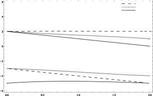
(a)  d=3

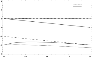
(b)  d=2

Figure 2: The Linear Pressure Model scaling exponents of the sectors $l=0$, $l=2$ and $l=4$ in three (a) and two (b) dimensions. The $z=0$ and $z=-d$ are omitted for the sake of clarity. We note that in two dimensions, there is a $z=2$ exponent in the $l=2$ sector but the $l=4$ sector’s exponent goes slightly above $z=2$.

We have plotted some of the poles in Fig. (2) in three dimensions. Remembering the $z=-3$ solution, we see that the anisotropic exponents are less dominant with increasing $l$ (a behavior repeated for higher $l$ as well).

V.1.1 Nonzero charge forcing

The contour bound is now $2-d-\xi<\mathcal{R}e(z)<0$, so there is no controversy in the choice of which poles to include. The small and large scale behaviors are similar to the passive scalar, and for completeness, we give the results in any dimension:

$$G_{ij}^{<} =AL^{2-\xi}\delta_{ij}-Br^{2-\xi}\mathcal{P}_{ij}(2-\xi)$$

$$G_{ij}^{>} =A^{\prime}L^{2-\xi}|r/L|^{2-d-\xi}\mathcal{P}_{ij}(2-d-\xi).$$ (75)

The $A,B$ and $A^{\prime}$ are somewhat complicated transcendental functions of $d$ and $\xi$.

V.1.2 Zero charge forcing

Now the forcing contributes a pole $\propto 1/(z+\xi+d)$ and the contour bound is $-d-\xi<\mathcal{R}e(z)<0$. The quantity $\gamma_{0}$ in eq. (72) has a zero there that cancels with the pole from the forcing. Therefore we again conclude that the forcing doesn’t contribute in the scaling. The small scale behavior is therefore same as above, but the large scale isotropic sector of the correlation function behaves as

$$G_{ij}^{>}=C^{\prime}|L|^{2-\xi}\left(A^{\prime}|r/L|^{-d}\mathcal{P}_{ij}(-d)+B^{\prime}|r/L|^{z_{-}}\mathcal{P}_{ij}(z_{-})\right)\!,$$ (76)

where $A^{\prime}$ and $B^{\prime}$ are again some nonzero constants (depending of $d$ and $\xi$), $z_{-}$ is the $l=2$ large scale mode (see Fig. (2)) and we have the traceless tensor

$$\mathcal{P}_{ij}(-d)=d\hat{\bm{r}}_{i}\hat{\bm{r}}_{j}-\delta_{ij}.$$ (77)

By looking at Fig. (2) we observe that the subleading exponent $z_{-}$ is smaller than the anisotropic exponent $l=2$ in three dimensions and $l=4$ at two dimensions (except when $\xi$ is close to two, when the $l=2$ exponent is larger than the $l=4$ exponent). Therefore the trace of the correlation function is dominated by the anisotropic modes.

VI Linearized Navier-Stokes equation

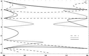
(a)  d=3

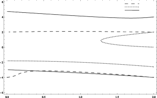
(b)  d=2

Figure 3: The Linearized Navier-Stokes equation exponents for sectors $l=0$, $l=2$ and $l=4$ (the legend applies to both figures) at three and two dimensions. In (a) the $l=4$ curves run slightly below and above the curves $z=-3-\xi$ and $z=2$, respectively. Other than leading exponents are also displayed.

Setting $a=-1$ in eq. (1) yields the Linearized Navier-Stokes equation (see e.g. frisch ; frisch.paper ; landau ). The equation may be considered as zeroth order perturbation theory of the full Navier-Stokes turbulence problem, from which one can at least in principle proceed to higher orders in perturbation theory. It will also serve as a stability problem where the background flow is determined by the Kraichnan ensemble instead of a solution to the Navier-Stokes equation (see chapter III of landau ). Not much is known of this case, except for the perturbative results in paolo ; jurc1 . The eq. (33) becomes

$$\frac{1}{\gamma_{-1}(z)}=d(d+2+\xi)\Gamma\left(1+\xi/2\right)\Gamma\left(1+d/2\right)$$

$$-2p_{\footnotesize{-1}}(z)\frac{\Gamma\left(-z/2\right)\Gamma\left(\frac{d+z+\xi}{2}\right)\Gamma\left(\frac{4+d-\xi}{2}\right)}{\Gamma\left(\frac{2+d+z}{2}\right)\Gamma\left(\frac{4-z-\xi}{2}\right)},$$

with

$$p_{-1}(z) =(z+\xi-2)\left(d^{2}(z+\xi)-(z+\xi)^{2}+d(z-1)z+d(\xi-1)\xi\right)-4(d+1)\xi z.$$ (78)

We choose to save space by not writing down explicitly the determinant for the anisotropic sectors. The expression may be reproduced by using the results of appendix C. We will also refrain from explicitly writing down expressions for the correlation functions, as it turns out that whichever sector has the leading exponents varies quite a bit with different values of $\xi$.

VI.1 d=3 with zero charge forcing

The contour bound is, as usual, $-3-\xi<\mathcal{R}e(z)<0$ and again one observes a cancelation of the corresponding pole. Inspecting Fig. (3) one observes quite wild behavior of the various scaling exponents at a first few sectors. A notable similarity to the three dimensional MHD case ($a=1$) are the exponents starting at $0$ and $-3$ and joining at $\xi\approx 0,35$. However in the LNS case one also sees similar behavior near $\xi=2$. Indeed one is tempted to assume the existence of a steady state only for $\xi$ near zero and two. The same conclusion could be drawn for the anisotropic sectors as well. We will further discuss this at the end of the paper. We will be satisfied with only reporting the scaling behaviors as the procedure for finding them is close to above cases. Assuming the steady state exists for $\xi$ close enough to zero and two, we conclude that for $\xi$ near zero, the small and large scale are dominated by the isotropic exponents starting at $0$ and $-3$, respectively. For $\xi$ near $2$, one instead observes $l=2$ dominance at small scales and $l=4$ dominance at large scales. We have deliberately neglected the nonzero charge forcing, as that would only bring about the familiar nonanomalous $-1-\xi$ scaling at large scales.

VI.2 $d=2$ with zero charge forcing

The behavior of the scaling exponents are much nicer, as can be seen by looking at Fig. (3). For $0\leq\xi\lesssim 1,3$, we see the small scales dominated by the $l=4$ anisotropic sector, and the large scale by the $l=2$ sector. For other values of $\xi$ the $l=2$ anisotropic sector dominates the small scales as well. The $l>4$ anisotropic exponents are all subleading with respect to the ones in the figure, and indeed respect the usual hierarchy of exponents paolo . In any case, the isotropic exponent is subleading.

VII The effect of varying the parameter $a$

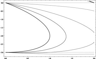
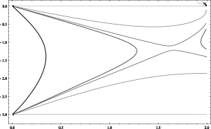
Figure 4: The leading isotropic exponents as $a$ is varied from $1$ to $0$ (a) and from $-1$ to $0$ (b) in three dimensions. The darkest curves correspond to $a=1$ and $a=-1$.

It is useful to discuss also other values of $a$ beside the discrete values $a=1,0,-1$. More specifically, looking at Fig. (4) we see how the closed contour determining the leading scaling exponents is deformed as $a$ varies from $a=1$ and $a=-1$ to $0$. Both end up as curves $z=0$ and $z=-3$. Also, as we know that when $a=1$ the steady state exists for $\xi<1$ in the isotropic sector vergassola (and for all $\xi$ in the anisotropic sectors arad ), it now seems even more reasonable to expect the steady state to exist for all $\xi$ in the $a=0$ case.

VIII Conclusion

The purpose of the present paper was to present an exact solution for the two point function of the so-called $a$ -model in the small and large scaling regimes, which incorporates the magnetohydrodynamic equations, the linear pressure model and the linearized Navier-Stokes equations. The phenomena of anomalous scaling and anisotropy dominance was investigated in each model with emphasis placed in the zero charge forcing concentrated at a finite wavenumber $\sim 1/L$ as in fouxon . Below we briefly summarize the findings in each model.

For the magnetohydrodynamic equations with $a=1$ the leading scaling behavior was observed to be anomalous and isotropic at both small and large scales in three dimensions for the zero charge forcing, in accordance with previous small scale results arad ; antonovlanottemazzino ; lanotte2 . In two dimensions with nonzero charge forcing one observes anomalous and anisotropic behavior at small scales, while the large scales are dominated by logarithmic behavior. The mechanism of the small scale anisotropy dominance is strikingly similar to the passive scalar large scale anisotropy dominance, except that in the MHD case the phenomenon results from the nonzero charge forcing. The zero charge forcing case in two dimensions is in agreement with the results in vergassola .

For the linear pressure model with $a=0$ and zero charge we recovered the small scale exponents of adz . The small scale behavior is now dominated by the isotropic and canonical scaling exponent $z=2-\xi$ (neglecting the constant mode by considering the structure function). The large scale behavior was seen to be dominated by a curious isotropic zero mode $z=-d$, although the trace of the structure function exhibits anomalous and anisotropic behavior at large scales. The nonzero charge forcing simply renders the large scale behavior canonical. The existence of the steady state is nevertheless controversial in two dimensions and requires further study.

The linearized Navier-Stokes equations corresponding to $a=-1$ seem to be the most interesting of the models considered, even more so because it is also the least well known. There still remains the question of the existence of the steady state, without which one cannot claim to have completely solved the problem. One may however conjecture it’s existence at least for small enough $\xi$ (at least in the isotropic sector), in which case the small and large scales are dominated by the isotropic anomalous scaling exponents in three dimensions. In two dimensions, the small scale exponents coincide with the somewhat rough numerical estimates of yoshida , the difference now being the absence of the scaling $\propto r^{-\xi}$ due to the forcing. Indeed, it was observed that both the small and large scales were dominated by anomalous anisotropic scaling exponents.

Although the linear equations above with the somewhat crude Kraichnan model are certainly some distance from the real problem of turbulence, similar scaling behavior has been observed in real and numerical simulations (see e.g. experimental ; experimental2 and references therein), namely implying that the scaling exponents in each anisotropic sector are universal as outlined above. Probably the closest case to the real Navier-Stokes turbulence is the linearized Navier-Stokes equation. The equation arises usually as one tries to verify the stability of a given stationary flow by decomposing the velocity field as $v+u$, where $v$ is the stationary, time independent term and $u$ is a small perturbation landau . If one can show that $u$ decays in time, the velocity field $v$ is indeed a laminar, stable flow. In our case $v$ is determined by the Kraichnan model and we are now concerned with the stability of the statistical steady state. It has been pointed out in jurc1 that in such a case one might be able to show that higher order perturbative terms are irrelevant in the sense of the renormalization group, thus implying that the steady state is in fact in the same universality class as the full NS turbulence. This would mean that the anomalous scaling exponent of the linear model is equal to the NS turbulence exponent. All this would of course depend on the existence of the steady state for $u$. Unfortunately it seems that such a steady state does not exist for the exponent $\xi=2/3$, which could be a sign of incompleteness of the Kraichnan model or a symptom of the general complexity of the problem of turbulence. The stability and existence problem will be studied more carefully in a future paper by the present author.

Appendix A Equation of motion for the pair correlation function

We take the Fourier transform of equation (1) and rewrite it as a stochastic partial differential equation of Stratonovich type as

$$d\widehat{u}_{i}(\bm{p})=\nu p^{2}\widehat{u}_{i}(\bm{p})dt-\widehat{\mathcal{D}}_{i\mu\nu}^{p}\!\int\!\!{\mathchar 22\relax\mkern-12.0mud}^{d}\bm{q}d\widehat{V}_{\nu}(\bm{q})\circ\widehat{u}_{\mu}(\bm{p}-\bm{q})+d\widehat{F}_{i}(\bm{p}),$$ (79)

where we have dropped the $t$ -dependence and denoted

$$\widehat{\mathcal{D}}_{iab}^{p}=i\left(\delta_{ia}p_{b}-a\delta_{ib}p_{a}\right)+i(a-1)p_{i}p_{a}p_{b}/p^{2}$$ (80)

and defined the Stratonovich product

$$d\widehat{V}_{\nu}(\bm{q})\circ\widehat{u}_{\mu}(\bm{p}-\bm{q})=d\widehat{V}_{\nu}(t,\bm{q})\widehat{u}_{\mu}(t+\frac{dt}{2},\bm{p}-\bm{q}).$$ (81)

As argued in zinn-justin by physical grounds, the symmetric prescription $\theta(0)=1/2$, corresponding to the Stratonovich definition of the SPDE, is the correct way of defining the equation. We will however use the relation $\widehat{u}_{\mu}(t+\frac{dt}{2},\bm{p})=\widehat{u}_{\mu}(t,\bm{p})+\frac{1}{2}d\widehat{u}_{\mu}(t,\bm{p})$ to transform the equation into a following Itô SPDE,

$$d\widehat{u}_{i}(\bm{p})=\nu p^{2}\widehat{u}_{i}(\bm{p})dt+\frac{1}{2}\widehat{\mathcal{D}}_{i\mu\nu}^{p}\!\int\!\!{\mathchar 22\relax\mkern-12.0mud}^{d}\bm{q}\widehat{D}_{\nu\sigma}(\bm{q})\widehat{\mathcal{D}}_{\mu\rho\sigma}^{p-q}\widehat{u}_{\rho}(\bm{p})$$

$$\ldots-\widehat{\mathcal{D}}_{i\mu\nu}^{p}\!\int\!\!{\mathchar 22\relax\mkern-12.0mud}^{d}\bm{q}d\widehat{V}_{\nu}(\bm{q})\widehat{u}_{\mu}(\bm{p}-\bm{q})+d\widehat{F}_{i}(\bm{p}),$$ (82)

where we have used the relation

$$d\widehat{V}_{i}(t,\bm{p})d\widehat{V}_{j}(t,\bm{p}^{\prime})=\widehat{D}_{ij}(\bm{p})\delta^{d}(\bm{p}+\bm{p}^{\prime})dt.$$ (83)

The first integral on the right hand side of the Itô SPDE can be done explicitly, resulting in

$$-\frac{1}{2}\widehat{\mathcal{D}}_{i\mu\nu}^{p}\!\int\!\!{\mathchar 22\relax\mkern-12.0mud}^{d}\bm{q}\widehat{D}_{\nu\sigma}(\bm{q})\widehat{\mathcal{D}}_{\mu\rho\sigma}^{p-q}\widehat{u}_{\rho}(\bm{p})=Dm_{v}^{-\xi}p^{2}\widehat{u}_{i}(\bm{p})+\widetilde{\lambda}p^{2-\xi}\widehat{u}_{i}(\bm{p})+\mathcal{O}(m_{v}^{+}),$$ (84)

where the incompressibility condition $p_{i}\widehat{u}_{i}(\bm{p})=0$ was used, and denoting

$$\widetilde{\lambda}=(a-1)\left(d+1+a(1-\xi)\right)\frac{d\pi\xi\csc(\pi\xi/2)\Gamma(d/2)c_{d}}{16\Gamma\left(\frac{d-\xi}{2}+2\right)\Gamma\left(\frac{d+\xi}{2}+1\right)}.$$ (85)

Applying the Itô formula to the quantity

$$\langle\widehat{u}_{i}(t,\bm{p})\widehat{u}_{j}(t,\bm{p}^{\prime})\rangle\doteq\widehat{G}_{ij}(t,\bm{p})\delta^{d}(\bm{p}+\bm{p}^{\prime})$$ (86)

and by assuming stationarity, one obtains the nonlocal PDE (with obvious $\bm{p}$ dependence omitted)

$$\left[2\nu-Dm_{v}^{-\xi}\right]|\bm{p}|^{2}\widehat{G}_{ij}-\widetilde{\lambda}D_{0}|\bm{p}|^{2-\xi}\widehat{G}_{ij}+\widehat{\mathcal{D}}_{i\mu\nu}^{p}\widehat{\mathcal{D}}_{j\rho\sigma}^{-p}\!\int\!\!{\mathchar 22\relax\mkern-12.0mud}^{d}\bm{q}\widehat{D}_{\nu\sigma}(\bm{q})\widehat{G}_{\mu\rho}(\bm{p}-\bm{q})=\widehat{C}_{ij}.$$ (87)

Using the $\mathrm{SO(d)}$ decomposition for $\widehat{G}$,

$$\widehat{G}_{ij}(\bm{p}):=\sum\limits_{a}B_{ij}^{a}(\hat{\bm{p}})\widehat{G}^{a}(p)$$ (88)

(and similarly for $\widehat{C}$), dividing the equation by $p^{2}$, and by taking the Mellin transform of the equation while remembering the definition

$$\widehat{G}_{ij}^{z}(\bm{p})=\int\limits_{0}^{\infty}\frac{dw}{w}w^{d+z}\widehat{G}_{ij}(w\bm{p})=|\bm{p}|^{-d-z}\sum\limits_{q}B_{ij}^{a}(\hat{\bm{p}})\bar{g}_{a}(z),$$ (89)

and by expressing $\widehat{D}$ in the integrand as an inverse Mellin transform, we finally obtain the equation

$$\left[2\nu-Dm_{v}^{-\xi}\right]\bar{g}_{b}(z)\!\!\!\!\!\! -\widetilde{\lambda}D_{0}\bar{g}_{b}(z-\xi)+\!\int\!\!{\mathchar 22\relax\mkern-12.0mud}z^{\prime}\bar{d}_{m_{v}}(z^{\prime})\mathrm{T}_{d+z^{\prime},d+z-z^{\prime}}^{bc}\bar{g}_{c}(z-z^{\prime})$$ (90)

$$=\bar{c}_{b}(z-2),$$

where we have defined (note the transpose in definition)

$$\sum\limits_{b}\mathrm{T}_{d+z^{\prime},d+z-z^{\prime}}^{cb}B_{ij}^{c}(\hat{\bm{p}})=|\bm{p}|^{d+z-2}\mathcal{D}_{i\mu\nu}^{\bm{p}}\mathcal{D}_{j\rho\sigma}^{-\bm{p}}\!\int\!\!{\mathchar 22\relax\mkern-12.0mud}^{d}\bm{q}\frac{P_{\nu\sigma}(\bm{p}-\bm{q})B_{\mu\rho}^{b}(\bm{q})}{\left|\bm{p}-\bm{q}\right|^{d+z^{\prime}}\left|\bm{q}\right|^{d+z-z^{\prime}}},$$ (91)

with the strips of analyticity,

$$\mathcal{R}e(z)-\mathcal{R}e(z^{\prime}) <0$$

$$\mathcal{R}e(z^{\prime}) <0$$

$$d+\mathcal{R}e(z) >0$$ (92)

such that the $9\times 9$ matrix $\mathbf{T}$ is independent of $\bm{p}$. The matrix elements $\mathrm{T}^{bc}$ can be determined exactly by computing the right hand side integral, which is the subject of the next appendix. As mentioned in sec. II.4, the first poles on the right occur at $z^{\prime}=0$ and $z^{\prime}=\xi$, which results in the equation in the limit of vanishing $m_{v}$:

$$2\nu\bar{g}_{b}(z)-D_{0}\widetilde{\lambda}\bar{g}_{b}(z-\xi)\!\!\!\! +\ \bar{d}_{m_{v}}(0)\mathrm{R}^{bc}\bar{g}_{c}(z)-D_{0}\mathrm{T}^{bc}_{d+\xi,d+z-\xi}(z)\bar{g}_{c}(z-\xi)$$ (93)

$$=\bar{c}_{b}(z-2).$$

We have defined the residue matrix

$$\mathrm{R}^{bc}=\mathcal{R}\left(\mathrm{T}_{d+z^{\prime},d+z-z^{\prime}}^{bc}\right)|_{z^{\prime}=0}$$ (94)

and used the residue of the velocity correlation at $z^{\prime}=\xi$:

$$\mathcal{R}_{z^{\prime}=\xi}\left(\bar{d}_{m_{v}}(z^{\prime})\right)=-D_{0}.$$ (95)

Appendix B Incompressibility condition

The incompressibility condition for $u$ and $f$ amounts to requiring that the contraction of the covariances (20) with $\bm{p}$ is zero, i.e.

$$|\bm{p}|^{d+z+l}p_{i}\widehat{G}_{ij}^{z}(\bm{p}) =\left(p_{j}\bar{g}_{1}+lp_{j}\bar{g}_{3}+p_{j}\bar{g}_{4}\right)\Phi^{l}(\bm{p})+|\bm{p}|^{2}\left((l-1)\bar{g}_{2}\partial_{j}+\bar{g}_{3}\partial_{j}\right)\Phi^{l}(\bm{p})$$ (96)

$$\equiv 0,$$

which gives a system of equations

$$\bar{g}_{1}+l\bar{g}_{3}+\bar{g}_{4} =0$$

$$(l-1)\bar{g}_{2}+\bar{g}_{3} =0.$$ (97)

We can achieve this conveniently by defining a projection operator

$$\widehat{\mathbf{P}}=\begin{pmatrix}\mathbf{1}&0\\ \mathbf{X}&0\end{pmatrix},$$ (98)

where

$$\mathbf{X}=\begin{pmatrix}0&-(l-1)\\ -1&l(l-1)\end{pmatrix}.$$ (99)

The solution to eq. (97) (and a similar one for the forcing) can then be written conveniently as

$$\mathbf{\bar{g}}:=\begin{pmatrix}\mathbf{\bar{h}}\\ \mathbf{X}\cdot\mathbf{\bar{h}}\end{pmatrix};\mathbf{\bar{c}}:=\begin{pmatrix}\mathbf{\bar{f}}\\ \mathbf{X}\cdot\mathbf{\bar{f}}\end{pmatrix}.$$ (100)

We also rewrite the matrices $\mathbf{R}$ and $\mathbf{T}$ in block form as

$$\mathbf{R}=\begin{pmatrix}\mathbf{R}_{1}&\mathbf{R}_{2}\\ \mathbf{R}_{3}&\mathbf{R}_{4}\end{pmatrix};\mathbf{T}_{d+\xi,d+z}=\begin{pmatrix}\mathbf{A}&\mathbf{B}\\ \mathbf{C}&\mathbf{D}\end{pmatrix}.$$ (101)

Note the above definition of $\mathbf{T}$ with a translation $z\to z+\xi$. $\mathbf{R}$ is independent of $z$. By operating with $\mathbf{\widehat{P}}$ on eq. (27), we obtain the equations (after translation $z\to z+\xi$),

$$\left[2\nu\!-\!Dm_{v}^{-\xi}\right]\mathbf{\bar{h}}(z+\xi)\!+\bar{d}_{m_{v}}(0)\left(\mathbf{R}_{1}\!+\mathbf{R}_{2}\!\cdot\!\mathbf{X}\right)\!\mathbf{\bar{h}}(z+\xi)-\widetilde{\lambda}D_{0}\mathbf{\bar{h}}(z)-D_{0}\left(\mathbf{A}+\mathbf{B}\cdot\mathbf{X}\right)\mathbf{\bar{h}}(z)$$

$$=\mathbf{\bar{f}}(z+\xi-2)$$ (102)

and an identical one but multiplied by $\mathbf{X}$ from the left. Thus we see that we only need the upper 2 by 2 matrices from $\mathbf{T}$. By using the definition eq. (94) and the results for $\mathrm{T}^{ab}$ in appendix C, we obtain

$$\mathbf{R}_{1}+\mathbf{R}_{2}\cdot\mathbf{X}=-\frac{d-1}{\Gamma(d/2+1)}c_{d}\mathbf{1},$$ (103)

which results in a cancellation of the remaining mass dependent terms. The remaining equation depends now only on the physical diffusivity $\nu$. Solving the equation iteratively would amount to a series expansion in powers of $\nu$ or $\nu^{-1}$, but we shall only consider the $\nu\to 0$ limit, which produces the solution in eq. (27).

Appendix C Necessary components of the matrix $\mathbf{T}$

Due to incompressibility, only some of the components of $\mathbf{T}$ will be needed. Computing the integrals of the type in (91) can be performed by using the result

$$\int{\mathchar 22\relax\mkern-12.0mud}^{d}\bm{q}\frac{\Phi^{l}(\widehat{\bm{q}}\cdot\widehat{e})}{\left|\bm{q}\right|^{2\alpha}\left|\bm{p}-\bm{q}\right|^{2\beta}}=:\lambda_{2\alpha,2\beta}\left|\bm{p}\right|^{d-2(\alpha+\beta)}\Phi^{l}(\widehat{\bm{p}}\cdot\widehat{e}),$$ (104)

where we have denoted by $\widehat{\bm{q}}\cdot\widehat{e}$ the angle between $\bm{q}$ and the $z$ -axis and defined

$$\lambda_{2\alpha,2\beta}:=\frac{\Gamma(d/2+l-\alpha)\Gamma(d/2-\beta)\Gamma(\alpha+\beta-d/2)}{\Gamma(\alpha)\Gamma(\beta)\Gamma(d+l-\alpha-\beta)}.$$ (105)

The tensorial structure can be obtained by partial integrations and by taking derivatives in $\bm{p}$. We will further define (note the transpose in the definition)

$$\mathrm{T}^{ab}_{d+\xi,d+z}:=\frac{\lambda_{l+d+z,d+\xi}}{d+\xi}\tau^{ab}(z).$$ (106)

The necessary components of $\tau$ are (others do not contribute due to the incompressibility condition):

$$\tau^{11} =\frac{(1+a^{2})(d-1)(l-z)-a^{2}\xi(z+d+\xi-l)}{(l-z-\xi)}+\frac{l(l-1)\xi}{(l-z-\xi)(l+z+d+\xi-2)}$$

$$\tau^{12} =\frac{a^{2}\xi}{(l-z-\xi)(l+z+d+\xi-2)}$$

$$\tau^{21} =a^{2}l(l-1)\frac{l+z+d-2}{l+z+d+\xi-2}\left(d-1+\xi\frac{z-l+d+\xi+2}{z-l+2}\right)$$

$$\tau^{22} =\frac{(d-1)(l+z+d-2)}{l+z+d+\xi-2}+\frac{(l-2)\xi\left(a^{2}(l-3)+2a(z+d+1)+l-3\right)}{(l-z-2)(l+z+d+\xi-2)}$$

$$+\frac{(a-1)^{2}(2-\xi)\xi(l^{2}-5l+6)}{(l-z-2)(l+z+d+\xi-2)(l+z+d+\xi-4)}$$

$$\tau^{31} =\frac{2al\xi(z+d+\xi-1)}{(l-z-\xi)(l+z+d+\xi-2)}+2a^{2}l\left(\frac{z+l(d+\xi-1)-(d+\xi)(z+\xi)}{l-z-\xi}\right.$$

$$\left.-\frac{(l-1)\xi(d+\xi-1)}{(l-z-\xi)(l+z+d+\xi-2)}-\frac{(l-1)(2-\xi)(d+\xi)\xi}{(l-z-2)(l-z-\xi)(l+z+d+\xi-2)}\right)$$

$$\tau^{32} =2\xi\frac{a\left(d-1+a(l-2)+z+\xi\right)-d-1}{(l-z-\xi)(l+z+d+\xi-2)}+\frac{4a(l-2)(2-\xi)\xi}{(l-z-2)(l-z-\xi)(l+z+d+\xi-2)}$$

$$+\frac{2\xi(a-1)^{2}\left(l^{2}-5l+6\right)(2-\xi)}{(l-z-2)(l-z-\xi)(l+z+d+\xi-4)(l+z+d+\xi-2)}$$

$$\tau^{41} =\frac{a^{2}\left((d+\xi)(z+\xi)-l(d+\xi-1)-z\right)-2a\xi}{l-z-\xi}+$$

$$+\xi\frac{d+1+2a(l-1)+a^{2}(1+2d-d^{2}-\xi(d-1))}{(l+z+d)(l-z-\xi)}+\frac{(a-1)^{2}(d+1)(2-\xi)\xi}{(l+z+d)(l-z-\xi)(l+z+d+\xi-2)}$$

$$-(2-\xi)\xi\frac{(a-1)^{2}\left(d^{2}+l(l+1)\right)+d\left((1+2l)(1-2a)+a^{2}(1+3l-l^{2})\right)}{(l-z-2)(l+z+d)(l-z-\xi)(l+z+d+\xi-2)}$$

$$+\frac{2(a-1)^{2}(d+l)(d+1+l)\xi(\xi^{2}-6\xi+8)}{(l-z-2)(l+z+d)(l-z-\xi+2)(l-z-\xi)(l+z+d+\xi-2)}$$

$$\tau^{42} =\frac{a\xi\left(a(l+z+d)-2(2-\xi)\right)}{(l+z+d)(l-z-\xi)(l+z+d+\xi-2)}-\frac{(2-\xi)\xi\left(d+3-2a(d+1+l)+a^{2}(d+3)\right)}{(l-z-2)(l+z+d)(l-z-\xi)(l+z+d+\xi-2)}$$ (107)

$$+\frac{(a-1)^{2}\xi(d+3)(8-6\xi+\xi^{2})}{(l-z-2)(l+z+d)(l-z-\xi)(l-z-\xi+2)(l+z+d+\xi-2)}$$

$$+\frac{(a-1)^{2}\xi(6-5l+l^{2})(8-6\xi+\xi^{2})}{(l-z-2)(l+z+d)(l-z-\xi)(l-z-\xi+2)(l+z+d+\xi-4)(l+z+d+\xi-2)}.$$

Appendix D The matrix $\mathbf{\widehat{P}^{\text{T}}K}$

We defined the matrix $\mathbf{K}$ as

$$\text{K}^{ab}B_{ij}^{b}(\hat{\bm{r}})=\!\int\!\!{\mathchar 22\relax\mkern-12.0mud}^{d}\bm{p}e^{i\bm{p}\cdot\bm{r}}\frac{B_{ij}^{a,l}(\hat{\bm{p}})}{|\bm{p}|^{d+z}},$$ (108)

where the elements are obtained by direct computation. Multiplication with the transpose of the projector (98) yields

$$\mathbf{P}^{\text{T}}\mathbf{K}=\imath 2^{-z}\frac{\Gamma\left(\frac{l-z}{2}\right)}{\Gamma\left(\frac{d+l+z}{2}\right)}\kappa,$$ (109)

where $\kappa$ is now a $2\times 4$ matrix,

$$\kappa=\begin{pmatrix}1-\frac{1}{z+d+l}&\frac{-1}{(z+2-l)(z+d+l)}&\frac{-1}{z+d+l}&-\frac{z-l}{z+d+l}\\ \frac{l(l-1)}{z+d+l}&\frac{(z+d)^{2}-l}{(z+d+l)(z+2-l)}&z+d-1+\frac{l(l-1)}{z+d+l}&2(z-l)(z+d+l-2)+\frac{l(l-1)}{z+d+l}\end{pmatrix}.$$ (110)

References

- (1) L. Ts. Adzhemyan, N. V. Antonov, A. Mazzino, P. Muratore-Ginanneschi, and A. V. Runov. Pressure and intermittency in passive vector turbulence. EPL (Europhysics Letters), 55(6):801–806, 2001.
- (2) L. Ts. Adzhemyan, N. V. Antonov, and A. V. Runov. Anomalous scaling, nonlocality, and anisotropy in a model of the passively advected vector field. Phys. Rev. E, 64(4):046310, Sep 2001.
- (3) Luiza Angheluta, Roberto Benzi, Luca Biferale, Itamar Procaccia, and Federico Toschi. Anomalous scaling exponents in nonlinear models of turbulence. Physical Review Letters, 97(16):160601, 2006.
- (4) N. V. Antonov, Michal Hnatich, Juha Honkonen, and Marian Jurčišin. Turbulence with pressure: Anomalous scaling of a passive vector field. Phys. Rev. E, 68(4):046306, Oct 2003.
- (5) N. V. Antonov, A. Lanotte, and A. Mazzino. Persistence of small-scale anisotropies and anomalous scaling in a model of magnetohydrodynamics turbulence. Phys. Rev. E, 61(6):6586–6605, Jun 2000.
- (6) I. Arad, L. Biferale, and I. Procaccia. Nonperturbative spectrum of anomalous scaling exponents in the anisotropic sectors of passively advected magnetic fields. Phys. Rev. E, 61(3):2654–2662, Mar 2000.
- (7) Itai Arad, Luca Biferale, Irene Mazzitelli, and Itamar Procaccia. Disentangling scaling properties in anisotropic and inhomogeneous turbulence. Phys. Rev. Lett., 82(25):5040–5043, Jun 1999.
- (8) Itai Arad, Brindesh Dhruva, Susan Kurien, Victor S. L’vov, Itamar Procaccia, and K. R. Sreenivasan. Extraction of anisotropic contributions in turbulent flows. Phys. Rev. Lett., 81(24):5330–5333, Dec 1998.
- (9) Itai Arad, Victor S. L’vov, and Itamar Procaccia. Correlation functions in isotropic and anisotropic turbulence: The role of the symmetry group. Phys. Rev. E, 59(6):6753–6765, Jun 1999.
- (10) H. Arponen and P. Horvai. Dynamo effect in the kraichnan magnetohydrodynamic turbulence. J. Stat. Phys., 129(2):205–239, Oct 2007.
- (11) R. Benzi, L. Biferale, and F. Toschi. Universality in passively advected hydrodynamic fields: the case of a passive vector with pressure. The European Physical Journal B, 24:125, 2001.
- (12) D. Bernard, K. Gawȩdzki, and A. Kupiainen. Slow modes in passive advection. J. Stat. Phys., 90(3):519–569, Feb 1998.
- (13) J. Bertrand, P. Bertrand, and J. Ovarlez. ÃÂThe Mellin Transform.ÃÂ The Transforms and Applications Handbook: Second Edition. CRC Press LLC, 2000.
- (14) A. Celani and A. Seminara. Large-scale anisotropy in scalar turbulence. Physical Review Letters, 96(18):184501, 2006.
- (15) G. Falkovich and A. Fouxon. Anomalous scaling of a passive scalar in turbulence and in equilibrium. Physical Review Letters, 94(21):214502, 2005.
- (16) G. Falkovich, K. Gawȩdzki, and M. Vergassola. Particles and fields in fluid turbulence. Rev. Mod. Phys., 73(4):913–975, Nov 2001.
- (17) U. Frisch. Turbulence: The Legacy of A. N. Kolmogorov. Cambridge University Press, 1995.
- (18) U. Frisch, Z. S. She, and P. L. Sulem. Large-scale flow driven by the anisotropic kinetic alpha effect. Physica D: Nonlinear Phenomena, 28(3):382–392, 1987.
- (19) K. Gawȩdzki and A. Kupiainen. Anomalous scaling of the passive scalar. Phys. Rev. Lett., 75(21):3834–3837, Nov 1995.
- (20) V. Hakulinen. Passive advection and the degenerate elliptic operators . Communications in Mathematical Physics, 235(1):1, 2003.
- (21) M. Hnatich, J. Honkonen, M. Jurcisin, A. Mazzino, and S. Sprinc. Anomalous scaling of passively advected magnetic field in the presence of strong anisotropy. Physical Review E (Statistical, Nonlinear, and Soft Matter Physics), 71(6):066312, 2005.
- (22) Robert H. Kraichnan. Anomalous scaling of a randomly advected passive scalar. Phys. Rev. Lett., 72(7):1016–1019, Feb 1994.
- (23) A. Kupiainen and P. Muratore-Ginanneschi. Scaling, renormalization and statistical conservation laws in the kraichnan model of turbulent advection. J. Stat. Phys., 126(3):669–724, Feb 2007.
- (24) L. D. Landau. Fluid Mechanics, 2nd. edition, Volume 6. Elsevier, 1987.
- (25) Alessandra Lanotte and Andrea Mazzino. Anisotropic nonperturbative zero modes for passively advected magnetic fields. Phys. Rev. E, 60(4):R3483–R3486, Oct 1999.
- (26) M. Vergassola. Anomalous scaling for passively advected magnetic fields. Phys. Rev. E, 53(4):R3021–R3024, Apr 1996.
- (27) K. Yoshida and Y. Kaneda. Anomalous scaling of anisotropy of second-order moments in a model of a randomly advected solenoidal vector field. Phys. Rev. E, 63(1):016308, Dec 2000.
- (28) J. Zinn-Justin. Quantum Field Theory and Critical Phenomena, 3rd ed. Oxford University Press, 1996.