Amplitude-Phase Coupling in a Spin-Torque Nano-Oscillator

Abstract

The spin-torque nano-oscillator in the presence of thermal fluctuation is described by the normal form of the Hopf bifurcation with an additive white noise. By the application of the reduction method, the amplitude-phase coupling factor, which has a significant effect on the power spectrum of the spin-torque nano-oscillator, is calculated from the Landau-Lifshitz-Gilbert-Slonczewski equation with the nonlinear Gilbert damping. The amplitude-phase coupling factor exhibits a large variation depending on in-plane anisotropy under the practical external fields.

When a direct current $I$ flows into a magnetoresistive (MR) device, a stationary magnetic state becomes unstable and a steady magnetic oscillation is excited by the spin-transfer torque. The oscillation is expected to be applicable to a nanoscale microwave source, i.e., the spin-torque nano-oscillator (STNO).Kiselev ; Rippard According to the theory based on the spin-wave Hamiltonian formalism,Slavin ; Tiberkevich ; Kim ; Kim2 the frequency nonlinearity plays a key role in determining the behavior of the oscillator. It has been shown that the strong frequency nonlinearity leads to significant effects on the power spectrum of STNO in the presence of thermal fluctuation: a linewidth enhancementKim and non-Lorentzian lineshapesKim2 . In this paper, the important nonlinearity is examined. From the Landau-Lifshitz-Gilbert-Slonczewski (LLGS) equation as the model of STNO, we calculate explicitly the magnitude of the quantity corresponding to the normalized frequency nonlinearity $N/\Gamma_{\mathrm{eff}}$ (see, e.g., Eq. (4) in Ref. Kim2, ) of the spin-wave approach. In particular, we take account of in-plane anisotropy of a magnetic film which has been neglected in the early studiesSlavin ; Tiberkevich ; Kim ; Kim2 , finding the large effect of the anisotropy on the nonlinearity.

We describe STNO by a generic oscillator model. It is known that small-amplitude oscillations near the Hopf bifurcation point are generally governed by the simple evolution equation for a complex variable $W(t)$ known as the Stuart-Landau (SL) equation.Kuramoto The SL equation is derived as a normal form of the supercritical Hopf bifurcation from the general system of ordinary differential equations. Accordingly, the LLGS equation similarly reduces to the SL equation in the case where the Hopf bifurcation, which represents a generation of magnetic oscillations in STNO, occurs. The reduction of the LLGS equation can be executed by the reduction method based on the center-manifold theorem. At finite temperature, there exists inevitable thermal magnetization fluctuation in STNO.Kim3 ; Mizushima We include the thermal effect into the magnetization dynamics by just adding white noise term to the SL equation, i.e., STNO in the presence of thermal fluctuation is described by the ‘noisy’ Hopf normal form:

$$\frac{\mathrm{d}\tilde{W}}{\mathrm{d}\tilde{t}}=i\tilde{\Omega}\tilde{W}+(1+i\delta)(p-|\tilde{W}|^{2})\tilde{W}+\eta(\tilde{t}),$$ (1)

where $\tilde{W}$ is the normalized complex variable representing the amplitude and phase of a magnetization vector $\bm{M}$ (see Eq. (7) below). In Eq. (1), $\tilde{\Omega}$ represents a fundamental frequency, $\tilde{t}$ is a normalized dimensionless time, and $\eta(\tilde{t})$ is the zero-mean, white Gaussian noise with the only non-vanishing second moment given by $\langle\eta(\tilde{t})\bar{\eta}(\tilde{t}^{\prime})\rangle=4\delta(\tilde{t}-\tilde{t}^{\prime})$. $p$ is the bifurcation parameter. An oscillation is generated when $p$ becomes positive. In the context of STNO, $p\propto(I-I_{\mathrm{c}})$ where $I_{\mathrm{c}}$ is the threshold current. The parameter $\delta$ quantifies the coupling between the amplitude and phase fluctuations and is called the amplitude-phase coupling factor. It is $\delta$ that we calculate numerically in this paper and that corresponds to the normalized frequency nonlinearity $N/\Gamma_{\mathrm{eff}}$ of the spin-wave approach. The amplitude-phase coupling factor $\delta$ affects the power spectrum of an oscillator and leads to linewidth enhancement and non-Lorentzian lineshapes.Risken ; Gleeson Due to its effect, the factor $\delta$ is also called the linewidth enhancement factor.Henry Eq. (1) is often used as the simplest model of a noisy auto-oscillator in many fields, for example, electrical engineering, chemical reactions, optics, biology, and so on.Risken ; Haken Therefore, we can easily compare STNO with conventional oscillators and clarify its features.

The amplitude-phase coupling factor $\delta$ is obtained in the procedure of the reduction of the LLGS equation. In the following, we first explain the LLGS equation. Then, following Kuramoto’s monographKuramoto , we consider an instability of a steady solution and execute the reduction of the LLGS equation.

The magnetic energy density of the free layer of STNO is assumed to have the form

$$\mathcal{E}=-\bm{M}\cdot\bm{H}_{\mathrm{ext}}-\frac{K_{\mathrm{u}}}{M_{\mathrm{s}}^{2}}(\bm{M}\cdot\hat{\bm{x}})^{2}+\frac{1}{2}4\pi\bm{M}\cdot\mathcal{N}\cdot\bm{M},$$ (2)

where $M_{\mathrm{s}}$ is the saturation magnetization, $\bm{H}_{\mathrm{ext}}=H_{x}\hat{\bm{x}}+H_{y}\hat{\bm{y}}+H_{z}\hat{\bm{z}}$ is an external field, $K_{\mathrm{u}}$ is uniaxial anisotropy along the $x$ direction, and $\mathcal{N}$ is the demagnetizing tensor; $\mathcal{N}=\mathrm{diag}(N_{x},N_{y},N_{z})$. Using the spherical coordinate system (see Fig. 1), we describe the magnetization dynamics of STNO by the LLGS equation

$$\begin{cases}\cos\psi~{}\dot{\phi}=-\alpha(\xi)\dot{\psi}-F_{1}(\phi,\psi,\omega_{J})\\ \dot{\psi}=\alpha(\xi)\cos\psi~{}\dot{\phi}+F_{2}(\phi,\psi,\omega_{J})\end{cases},$$ (3)

where $F_{1}(\phi,\psi,\omega_{J})\equiv(\gamma/M_{\mathrm{s}})\partial\mathcal{E}/\partial\psi-a(\phi,\omega_{J})$ and $F_{2}(\phi,\psi,\omega_{J})\equiv(\gamma/(M_{\mathrm{s}}\cos\psi))\partial\mathcal{E}/\partial\phi+b(\phi,\psi,\omega_{J})$. $\gamma$ is the gyromagnetic ratio. The second terms of $F_{i}$ result from the Slonczewski term $\bm{T}_{J}=(\gamma a_{J}/M_{\mathrm{s}})\bm{M}\times(\bm{M}\times\bm{p})$ in which $a_{J}$ is proportional to the current density $J$ through the free layerSlonczewski . Therefore, $a(\phi,\omega_{J})\equiv\omega_{J}\cos\psi_{\mathrm{p}}\sin(\phi-\phi_{\mathrm{p}})$ and $b(\phi,\psi,\omega_{J})\equiv\omega_{J}[\cos\psi_{\mathrm{p}}\sin\psi\cos(\phi-\phi_{\mathrm{p}})-\sin\psi_{\mathrm{p}}\cos\psi]$, where $\omega_{J}=\gamma a_{J}$. $\alpha(\xi)$-terms of Eqs. (3) are the generalized Gilbert damping terms proposed by Tiberkevich and Slavin.Tiberkevich2 We take into account only the first non-trivial term of the Taylor series expansion for $\alpha(\xi)$ by the magnetization change rate $\xi\equiv(\partial\bm{m}/\partial t)^{2}/(\gamma 4\pi M_{\mathrm{s}})^{2}$; $\alpha(\xi)=\alpha_{\mathrm{G}}(1+q_{1}\xi)$. According to Ref. Tiberkevich2, , the nonlinear LLGS model with $q_{1}=3$ gives a good agreement with the experimental results of Ref. Kiselev, and Ref. Mistral, .

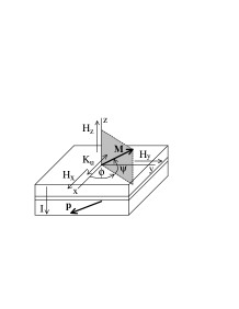
Figure 1: The spherical coordinate system $(\phi,\psi)$ for the direction of the free layer magnetization $\bm{m}=\bm{M}/M_{\mathrm{s}}$ of STNO. $\bm{p}$ denotes the direction of the pinned layer magnetization; $\bm{p}=(\cos\psi_{\mathrm{p}}\cos\phi_{\mathrm{p}},\cos\psi_{\mathrm{p}}\sin\phi_{\mathrm{p}},\sin\psi_{\mathrm{p}})$.

An instability of a steady solution of Eq. (3) is considered. A steady solution $(\phi_{0}(\omega_{J}),\psi_{0}(\omega_{J}))$ is derived from $F_{i}(\phi_{0},\psi_{0},\omega_{J})=0$. Shifting the variables as $u_{1}\equiv\phi-\phi_{0}$ and $u_{2}\equiv\psi-\psi_{0}$, we have the Taylor series of Eq. (3) as follows,

$$\dot{\bm{u}}=L\bm{u}+N_{2}\bm{u}\bm{u}+N_{3}\bm{u}\bm{u}\bm{u}+\cdots$$ (4)

where $\bm{u}=(u_{1},u_{2})^{\mathrm{T}}$. Here, the diadic and triadic notations Kuramoto have been used. The stability of a steady solution is determined by the eigenvalues of the linear coefficient matrix $L$: $\lambda_{\pm}=\Gamma\pm(\Gamma^{2}-\det L)^{1/2}$. $\Gamma$ is defined as $\Gamma=\Gamma(\omega_{J})\equiv(1/2)\mathrm{tr}L$ and plays the role as a control parameter since it depends on $\omega_{J}$. We confine ourselves to the case where the Hopf bifurcation occurs. Then, $\lambda_{\pm}$ is a pair of complex-conjugate eigenvalues. The point, $\Gamma=0$, is the Hopf bifurcation point; while a steady solution remains stable for $\Gamma<0$, it becomes unstable for $\Gamma>0$. The bifurcation point corresponds to the threshold $\omega_{J}^{\mathrm{c}}$ which is determined by $\mathrm{tr}L=0$ and $F_{i}(\phi_{0},\psi_{0},\omega_{J}^{\mathrm{c}})=0$. Near the bifurcation point, we divide $L$ into the two parts; $L=L_{0}+\Gamma L_{1}$, where $L_{0}$ is the critical part and $\Gamma L_{1}$ is the remaining part. Corresponding to $L$, $\lambda_{+}$ is also divided into the two parts; $\lambda_{+}=\lambda_{0}+\Gamma\lambda_{1}$. Although $L_{1}$ and $\lambda_{1}$ generally depend on $\Gamma$ further, we neglect their dependence and evaluate them by the values at $\Gamma=0$. Accordingly, $\lambda_{0}=i\omega_{0}$ and

$$\lambda_{1}=1-\frac{1}{2i\omega_{0}}\left.\frac{\mathrm{d}}{\mathrm{d}\Gamma}\det L\right|_{\Gamma=0},$$ (5)

where $\omega_{0}\equiv\sqrt{\det L_{0}}$. The right and left eigenvector of $L_{0}$ corresponding to the eigenvalue $\lambda_{0}$ are denoted as $\bm{U}$ and $\bm{U}^{\ast}$, respectively. These are normalized as $\bm{U}^{\ast}\bm{U}=\bar{\bm{U}^{\ast}}\bar{\bm{U}}=1$ where $\bar{\bm{U}}$ means a complex conjugate of $\bm{U}$.

Let us apply the reduction method to Eq. (4). The SL equation for a complex amplitude $W(t)$,

$$\dot{W}=\Gamma\lambda_{1}W-g|W|^{2}W$$ (6)

and the neutral solution for the magnetization dynamics,

$$\begin{pmatrix}\phi\\ \psi\end{pmatrix}=\begin{pmatrix}\phi_{0}\\ \psi_{0}\end{pmatrix}+W(t)e^{i\omega_{0}t}\bm{U}+\bar{W}(t)e^{-i\omega_{0}t}\bar{\bm{U}}$$ (7)

are obtained within the lowest order approximation.Kuramoto Under the approximation, only the Taylor expansion coefficients up to the third order are needed. The complex constant $g$ in Eq. (6) is given by

$$\begin{split}g\equiv\nu_{1}+i\nu_{2}=&-3(\bm{U}^{\ast},N_{3}\bar{\bm{U}}\bm{U}\bm{U})\\ &+4(\bm{U}^{\ast},N_{2}\bm{U}\bm{V}_{0})+2(\bm{U}^{\ast},N_{2}\bar{\bm{U}}\bm{V}_{+}),\end{split}$$ (8)

where $\bm{V}_{0}=L_{0}^{-1}N_{2}\bm{U}\bar{\bm{U}}$ and $\bm{V}_{+}=(L_{0}-2i\omega_{0})^{-1}N_{2}\bm{U}\bm{U}$. The amplitude-phase coupling factor $\delta$ is obtained from the complex constant $g$ and is given by

$$\delta=\nu_{2}/\nu_{1}.$$ (9)

In this way, the factor $\delta$ for STNO can be calculated numerically from the parameters of the LLGS equation.

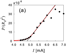
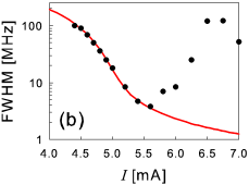
Figure 2: (Color online) (a) Power $P$ divided by $R_{0}I^{2}$ with $R_{0}=13.6~{}\Omega$ and (b) linewidth (FWHM) of the signal of STNO as a function of applied current $I$. Dots are experimental data at $T=150$ K taken from Ref. Mistral, . Red lines are theoretical fitting curves based on the model of Eq. (1).

The noisy Hopf normal form given by Eq. (1) is derived when we add the noise term $f(t)$ with $\langle f(t)\bar{f}(t^{\prime})\rangle=4D\gamma^{2}\delta(t-t^{\prime})$ to the SL Eq. (6). $f(t)$ has the dimension of frequency. The components in Eq. (1) are defined as $\tilde{W}(t)=(D\gamma^{2}/\nu_{1})^{-1/4}W(t)e^{i(\omega_{0}+\Gamma\delta-\Gamma\mathrm{Im}\lambda_{1})t}$, $\tilde{t}\equiv\sqrt{D\gamma^{2}\nu_{1}}t$, $p\equiv\Gamma/\sqrt{D\gamma^{2}\nu_{1}}$, and $\tilde{\Omega}\equiv\omega_{0}/\sqrt{D\gamma^{2}\nu_{1}}$. Therefore, we can make the most of many well-known properties of Eq. (1) Risken ; Gleeson to examine the behavior of STNO. It is known, for example, that the spectrum linewidth $\Delta\omega_{\mathrm{FWHM}}$ far above the threshold ($p\gg 0$) is increased by a factor of $(1+\delta^{2})$.Risken In the context of STNO, when $\Gamma\gg 0$, the linewidth can be expressed as

$$\Delta\omega_{\mathrm{FWHM}}=\Delta\omega_{\mathrm{res}}\times\frac{k_{\mathrm{B}}T}{E_{\mathrm{osci}}}\times\frac{1}{2}(1+\delta^{2}),$$ (10)

which corresponds to Eq. (11) in Ref. Kim, . Here, $k_{\mathrm{B}}T$ is the thermal energy. $\Delta\omega_{\mathrm{res}}$ is the linewidth at thermal equilibrium ($\omega_{J}=0$) given by $\Delta\omega_{\mathrm{res}}=2\Gamma_{\mathrm{eq}}$, where $\Gamma_{\mathrm{eq}}\equiv-\Gamma(\omega_{J}=0)$. Moreover, $E_{\mathrm{osci}}$ is the magnetization oscillating energy and can be written as $E_{\mathrm{osci}}\simeq 2\bm{U}^{\dagger}[\frac{\partial(\partial_{u_{1}}\mathcal{E},\partial_{u_{2}}\mathcal{E})}{\partial(u_{1},u_{2})}]_{\bm{u}=\bm{0}}\bm{U}P_{W}V_{\mathrm{free}}=\frac{1}{2}\frac{\Gamma_{\mathrm{eq}}k_{\mathrm{B}}T}{D\gamma^{2}}P_{W}$ when it is assumed that $E_{\mathrm{osci}}\simeq k_{\mathrm{B}}T$ near thermal equilibrium (energy equipartition). Here, $V_{\mathrm{free}}$ is the volume of the free layer and $P_{W}$ is the total power of $W(t)$ given by $P_{W}=\sqrt{D\gamma^{2}/\nu_{1}}\{p+2/F(p)\}$ with $F(p)\equiv\sqrt{\pi}e^{p^{2}/4}[1+\mathrm{erf}(p/2)]$. From the expression of Eq. (10), it is found that the MR device in STNO itself is nothing but a resonator on the analogy of electrical circuits. The other one of well-known properties of Eq. (1) is that the amplitude-phase coupling factor distorts the power spectrum to non-Lorentzian lineshapes especially near the threshold (see, e.g., FIG. 5 of Ref. Gleeson, ). The degree of the lineshape distortion is determined by the magnitude of $\delta$ and $p$, corresponding to the calculation in Ref. Kim2, . We comment on the validity of Eq. (1) for large-amplitude oscillations. In Fig. 2, the theoretical fitting curves based on the model Eq. (1) are compared with the experimental data of Ref. Mistral, and give a good agreement with them up to $I\simeq 5.6$ mA ($p\simeq 8.2$) beyond the threshold current $I_{\mathrm{c}}=4.8$ mA ($p=0$) estimated by the fitting. note Therefore, although the derivation of Eq. (1) is based on a perturbation expansion around the bifurcation point, it is considered to be valid for rather large-amplitude oscillations with $p\sim 10$.

We briefly mention the oscillating frequency $\omega_{\mathrm{osci}}$. From Eqs. (1) and (7), the oscillating frequency of a free layer magnetization far above threshold is written as $\omega_{\mathrm{osci}}=\omega_{0}-\Gamma\delta+\Gamma\mathrm{Im}\lambda_{1}$. Although the calculation results for $\mathrm{Im}\lambda_{1}$ of Eq. (5) are not shown here, we have found that this quantity has a small value with $\mathrm{Im}\lambda_{1}\sim\alpha_{\mathrm{G}}$ for wide range of parameters of the LLGS equation. Accordingly, $\omega_{\mathrm{osci}}$ is approximately given by $\omega_{\mathrm{osci}}\simeq\omega_{0}-\Gamma\delta$. Since $\Gamma\propto(I-I_{\mathrm{c}})$, while the frequency $\omega_{\mathrm{osci}}$ decreases as the current $I(>I_{\mathrm{c}})$ increases when $\delta>0$ (red shift), $\omega_{\mathrm{osci}}$ increases when $\delta<0$ (blue shift) in accordance with the spin-wave models Slavin ; Tiberkevich ; Kim ; Kim2 .

Figure 3: (Color online) (a) Dependence of $\delta$ on the nonlinearity of the damping $q_{1}$ for various values of an external magnetic field $H$. An uniaxial anisotropy field is taken as $H_{k}/4\pi M_{\mathrm{s}}=0.04$. (b) Dependence of $\delta$ on an external magnetic field $H$ for various values of an uniaxial anisotropy field $H_{k}$.

As illustrated above, the amplitude-phase coupling factor $\delta$ plays a key role to determine the behavior of an oscillator. Therefore, the features of STNO can be found out by the calculation of $\delta$.

Some calculation examples of $\delta$ are shown in Fig. 3. It is considered the case where a free layer is an in-plane magnetic film with an in-plane external field applied along the $x$ direction, $\bm{H}_{\mathrm{ext}}=H\hat{\bm{x}}$. It is assumed that $\mathcal{N}=\mathrm{diag}(0,0,1)$, $\alpha_{\mathrm{G}}=0.02$, and $(\phi_{\mathrm{p}},\psi_{\mathrm{p}})=(0,0)$. In Fig. 3(a), the dependence of $\delta$ on the nonlinearity of the damping $q_{1}$ is shown. It is found that $\delta$ monotonically decreases for $q_{1}$ and the variation of $\delta$ is very large. This result suggests that a nonlinear damping significantly changes the LLG dynamics. Tiberkevich2 In Fig. 3(b), the dependence of $\delta$ on an external magnetic field $H$ for various values of an uniaxial anisotropy field $H_{k}(=2K_{\mathrm{u}}/M_{\mathrm{s}})$ is shown. The nonlinearity of the damping is taken as $q_{1}=3$.Tiberkevich2 In the practical external field region, $\delta$ is very sensitive to an uniaxial anisotropy field and varies largely. Therefore, when the dynamics of STNO is considered, it is necessary to take the effect of an uniaxial anisotropy field into account seriously. This is the main result of the present paper.

In summary, we have considered the dynamics of STNO by reducing the LLGS equation to a generic oscillator model and calculated explicitly the amplitude-phase coupling factor which is the key factor for the power spectrum. The amplitude-phase coupling factor $\delta$ is very sensitive to magnetic fields, in-plane anisotropy, and the nonlinearity of damping. The large variation of $\delta$ is the remarkable feature of STNO in comparison with conventional oscillators. The calculation way for $\delta$ shown is applicable for an arbitrary magnetization configuration and is useful for finding a stable STNO with small $\Delta\omega_{\mathrm{FWHM}}$ (Eq. (10)), which is preferable for applications.

References

- (1) S. I. Kiselev et al, Nature 425, 380 (2003).
- (2) W. H. Rippard et al, Phys. Rev. Lett. 92, 027201 (2004).
- (3) A. N. Slavin and P. Kabos, IEEE Trans. Magn. 41, 1264 (2005).
- (4) V. Tiberkevich, A. N. Slavin, and J.-V. Kim, Appl. Phys. Lett. 91, 192506 (2007).
- (5) J.-V. Kim, V. Tiberkevich, and A. N. Slavin, Phys. Rev. Lett. 100, 017207 (2008).
- (6) J.-V. Kim et al., Phys. Rev. Lett. 100, 167201 (2008).
- (7) Y. Kuramoto, Chap. 2 of Chemical Oscillations, Waves, and Turbulence (Springer-Verlag, Berlin, 1984).
- (8) J.-V. Kim, Phys. Rev. B 73, 174412 (2006).
- (9) K. Mizushima, K. Kudo, and R. Sato, J. Appl. Phys. 101, 113903 (2007).
- (10) H. Risken, Chap. 12 of Fokker-Planck Equation (2nd Ed. Springer-Verlag, Berlin, 1989).
- (11) J. P. Gleeson and F. O’Doherty, SIAM J. Appl. Math. 66, 1669 (2006).
- (12) C. H. Henry, IEEE Journal of Quantum Electronics, QE-18, 259 (1982).
- (13) H. Haken, Advanced Synergetics (Springer-Verlag, New York, 1993).
- (14) J. C. Slonczewski, J. Magn. Magn. Mater. , L1 (1996).
- (15) V. Tiberkevich and A. Slavin, Phys. Rev. B 75, 014440 (2007).
- (16) Q. Mistral et al., Appl. Phys. Lett. 88, 192507 (2006).
- (17) The dimensionless power in Fig. 2(a) is given by with and . To obtain the linewidth in Fig. 2(b), we have used the parameters of MHz and , and have solved the eigenvalue problem of the Fokker-Planck equation corresponding to Eq. (1) as done in Ref. Risken, or Ref. Kim2, .