Generating EPR beams in a cavity optomechanical system

Abstract

We propose a scheme to produce continuous variable entanglement between phase-quadrature amplitudes of two light modes in an optomechanical system. For proper driving power and detuning, the entanglement is insensitive with bath temperature and $Q$ of mechanical oscillator. Under realistic experimental conditions, we find that the entanglement could be very large even at room temperature.

Entanglement is the key resource of the field of quantum information. Light is the perfect medium to distribute entanglement among distant parties. Entangled light with continuous variable (CV) entanglement between phase-quadrature amplitudes of two light modes is widely used in teleportation, entanglement swap, dense coding, etc. Braunstein and Loock (2005). This type of entangled state is also called Einstein-Podolsky-Rosen (EPR) state. The EPR beams have been generated experimentally by a nondegenerate optical parameter amplifier Ou et al. (1992), or Kerr nonlinearity in an optical fiber Silberhorn et al. (2001). The later one is simpler and more reliable. The Kerr nonlinearity is used to generate two independent squeezed beams. With interference at a beam splitter, the EPR entanglement is obtained between output beams. However, Kerr nonlinearity in fiber is very weak, which limits entanglement between output beams.

It was found that strong Kerr nonlinearity appeared in an optomechanical system consisting of a cavity with a movable boundary Hilico and et al. (1992); Mancini and Tombesi (1994); Fabre et al. (1994). Besides, the single-mode squeezing could be made insensitive with thermal noise Mancini and Tombesi (1994), which makes the scheme very attractive. However, the frequency of output squeezed beams cannot be made identical, which makes interference difficult. Then it was generalized to two-mode schemes in order to generate EPR beams without interference Giovannetti et al. (2001); Mancini and Gatti (2001); Pirandola et al. (2003); Genes et al. (2008); Wipf et al. (2008). However, they are either very sensitive to thermal noises Giovannetti et al. (2001); Mancini and Gatti (2001); Genes et al. (2008); Wipf et al. (2008), or requiring ultrahigh mechanical oscillator Q $\sim 10^{8}$ to suppress thermal noise effects Pirandola et al. (2003), which is $2$ to $3$ orders higher than the present available parameters Regal1 et al. (2008). The practical scheme to generate EPR beams in an optomechanical system needs to overcome these problems.

In this paper we propose a practical scheme to produce EPR beams in an optomechanical system, which consists of a whispering-gallery mode(WGM) cavity with a movable boundary. We find that, similarly as the single-mode scheme Mancini and Tombesi (1994), the thermal noise in the two-mode scheme can be greatly suppressed by adiabatically eliminating an oscillator mode. By precisely tuning the laser power and detuning, the oscillation mode is adiabatically eliminated and two output sideband modes are entangled. Unlike the cavity-free scheme Pirandola et al. (2003), our scheme requires modest oscillator $Q$. Besides, the output light is continuous in our scheme, other than pulse in Ref. Pirandola et al. (2003). The most attractive feature of our scheme is that the entanglement between output beams is nearly not changed under different bath temperature and $Q$ of the mechanical oscillator. Within the experimentally available parameters Schliesser et al. (2008, 2008), we find the maximum two-mode squeezing could be higher than $16$ dB under room temperature. The entanglement of formation (EOF) between two modes is larger than $5$ Giedke et al. (2003). Since the coupling efficiency between cavity and fiber could be larger than $99\%$ in the WGM cavity system Spillane et al. (2003), we neglect the coupling induced noises in this paper.

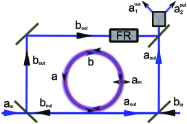
Figure 1: (Color online) Experimental setup. Cavity modes $a$ and $b$, which are driven by four lasers, couple to the mechanical mode $a_{m}$.

As shown in Fig. 1, we consider an optomechanical system consisting of a WGM cavity with a movable boundary. There are two cavity modes $a$ and $b$ with the same frequency but the opposite momentum. They are coupling with the same mechanical oscillation mode $a_{m}$ and driven by four lasers, two from the right-hand side with frequencies $\omega_{L}$ and $\omega_{L^{\prime}}$, the other two from the left-hand side with frequencies $\omega_{L}$ and $\omega_{L^{\prime}}$. $a_{\mathrm{in}}$ and $b_{\mathrm{in}}$ are input lights. $a_{1}^{\mathrm{out}}$ and $a_{2}^{\mathrm{out}}$ are output lights. Two lower mirrors have very high probability ($>99\%$) to reflect the driving lasers. So we neglect the reflecting induced noise for $a_{\mathrm{out}}$ and $b_{\mathrm{out}}$. The system Hamiltonian is $H=H_{0}+H_{d}+H_{I}$, where Wilson-Rae et al. (2007); Marquardt et al. (2007); Dayan et al. (2008); Srinivasan and Painter (2007)

$$H_{0}= \hbar\omega_{p}(a^{\dagger}a+b^{\dagger}b)+\hbar\omega_{m}a^{\dagger}_{m}a_{m}$$ (1)

$$H_{d}= \hbar(\frac{\Omega_{a}}{2}a+\frac{\Omega_{b}}{2}b)e^{-i\omega_{L}t}+\hbar(\frac{\Omega_{a}^{\prime}}{2}a+\frac{\Omega_{b}^{\prime}}{2}b)e^{-i\omega_{L}^{\prime}t}+\mathrm{H.c.}$$

$$H_{I}= \hbar\nu(a^{\dagger}b+ab^{\dagger})+\hbar\eta\omega_{m}(a^{\dagger}a+b^{\dagger}b)(a_{m}+a^{\dagger}_{m}).$$

Here $a$, $b$ and $a_{m}$ are the annihilation operators for the optical and mechanical modes, $\omega_{p}$ and $\omega_{m}$ are their angular frequency. $\Omega_{j}$ with $j=a,b$ is the driving amplitude and defined as $\Omega_{j}=2\sqrt{P_{j}/\hbar\omega_{L}\tau}$, where $P_{j}$ is the input laser power and $\tau=1/\gamma$ is the photon loss rate into the output modes. $\nu$ is the coupling strength between cavity modes $a$ and $b$. For the WGM cavity system, it ranges from $100$ MHz to $10$ GHz Dayan et al. (2008); Srinivasan and Painter (2007). The dimensionless parameter $\eta=(\omega_{p}/\omega_{m})(x_{m}/R)$ is used to characterize optomechanical coupling, with $x_{m}=\sqrt{\hbar/m\omega_{m}}$ the zero-point motion of the mechanical resonator mode Kippenberg and Vahala (2007), $m$ its effective mass, and $R$ a cavity radius. In typical WGM cavity systems we find $\eta\sim 10^{-4}$.

We define the normal modes $a_{1}=(a+b)/\sqrt{2}$ and $a_{2}=(a-b)/\sqrt{2}$. We suppose the conditions that $\Omega_{a}-\Omega_{b}=0$ and $\Omega_{a}^{\prime}+\Omega_{b}^{\prime}=0$ are satisfied. The Hamiltonian can be written as

$$H= \hbar(\omega_{p}+\nu)a_{1}^{\dagger}a_{1}+\hbar(\omega_{p}-\nu)a_{2}^{\dagger}a_{2}+\hbar\omega_{m}a_{m}^{\dagger}a_{m}$$ (2)

$$+\hbar(\frac{\Omega_{1}}{2}a_{1}e^{-i\omega_{L}t}+\frac{\Omega_{2}}{2}a_{2}e^{-i\omega_{L}^{\prime}t}+\mathrm{H.c.})$$

$$+\hbar\eta\omega_{m}(a_{1}^{\dagger}a_{1}+a_{2}^{\dagger}a_{2})(a_{m}^{\dagger}+a_{m}),$$

where $\Omega_{1}=\Omega_{a}+\Omega_{b}$ and $\Omega_{2}=\Omega_{a}^{\prime}-\Omega_{b}^{\prime}$. We define the detuning $\Delta_{1}=\omega_{L}-\omega_{p}-\nu$ and $\Delta_{2}=\omega_{L}^{\prime}-\omega_{p}+\nu$. As shown in Fig. 1, with beam splitters and Faraday rotator, we can get the output mode of $a_{1}$ and $a_{2}$. We assume both cavity and oscillator modes are weakly dissipating at rates $\gamma$ and $\gamma_{m}$, respectively, where $\gamma_{m}\ll\omega_{m}$. We can get quantum Langevin equations Walls and Milburn (1994)

$$\dot{a}_{j} = i\Delta_{j}a_{j}-i\eta\omega_{m}a_{j}(a_{m}+a^{\dagger}_{m})-i\frac{\Omega_{j}}{2}a_{j}-\frac{\gamma}{2}a_{j}(t)$$ (3)

$$+\sqrt{\gamma}a_{j}^{\mathrm{in}}~{}~{}\mathrm{for}~{}j=1,2,$$

$$\dot{a}_{m} = -i\eta\omega_{m}\sum_{j=1}^{2}a_{j}^{\dagger}a_{j}-(i\omega_{m}+\frac{\gamma_{m}}{2})a_{m}+\sqrt{\gamma_{m}}a_{m}^{\mathrm{in}},$$ (4)

where thermal noise inputs are defined as correlation functions $\langle a_{m}^{\mathrm{in}\dagger}(t),a_{m}^{\mathrm{in}}(t^{\prime})\rangle=n_{m}\delta(t-t^{\prime})$, $\langle a_{m}^{\mathrm{in}\dagger}(t),a_{m}^{\mathrm{in}\dagger}(t^{\prime})\rangle=\langle a_{m}^{\mathrm{in}}(t),a_{m}^{\mathrm{in}}(t^{\prime})\rangle=0$, $\langle a_{j}^{\mathrm{in}\dagger}(t),a_{j}^{\mathrm{in}}(t^{\prime})\rangle=\langle a_{j}^{\mathrm{in}\dagger}(t),a_{j}^{\mathrm{in}\dagger}(t^{\prime})\rangle=\langle a_{j}^{\mathrm{in}}(t),a_{j}^{\mathrm{in}}(t^{\prime})\rangle=0$, with $n_{m}$ the thermal occupancy number of thermal bath for oscillator mode. We suppose cavity modes couple with vacuum bath.

To simplify Eqs. (3) and (4), we apply a shift to normal coordinate, $a_{j}\rightarrow a_{j}+\alpha_{j}$, $a_{m}\rightarrow a_{m}+\beta$. $\alpha_{j}$ and $\beta$ are $c$ numbers, which are chosen to cancel all $c$ number terms in the transformed equations. We find they should fulfill the following requirements: $\beta\simeq-\eta(|\alpha_{1}|^{2}+|\alpha_{2}|^{2})$, and $i\Delta_{j}\alpha_{j}+2i\eta^{2}\omega_{m}\alpha_{j}(|\alpha_{1}|^{2}+|\alpha_{2}|^{2})-\frac{\gamma}{2}\alpha_{j}-i\frac{\Omega_{j}}{2}=0$. Because $\gamma_{m}\ll\omega_{m}$, the imaginary part of $\beta$ can be neglected. In the limit $\Delta_{j}\gg 2\eta^{2}w_{m}(|\alpha_{1}|^{2}+|\alpha_{2}|^{2})$, we find $\alpha_{j}\simeq\Omega_{j}/\sqrt{\gamma^{2}+4\Delta_{j}^{2}}$. In the limit $|\alpha|\gg|\langle a_{p}\rangle|$, the Langevin equations are linearized as

$$\dot{a}_{j} = -i\eta\omega_{m}\alpha_{j}(a_{m}+a_{m}^{\dagger})+(i\Delta_{j}^{\prime}-\frac{\gamma}{2})a_{j}+\sqrt{\gamma}a_{j}^{\mathrm{in}},$$ (5)

$$\dot{a}_{m} = -i\eta\omega_{m}\sum_{p=1}^{2}(\alpha_{p}^{*}a_{p}+\alpha_{p}a_{p}^{\dagger})-(i\omega_{m}+\frac{\gamma_{m}}{2})a_{m}$$ (6)

$$+\sqrt{\gamma_{m}}a_{m}^{\mathrm{in}},$$

where $j=1,2$ and $\Delta_{j}^{\prime}=\Delta_{j}+2\eta^{2}\omega_{m}(|\alpha_{1}|^{2}+|\alpha_{2}|^{2})$. We suppose $\Delta_{1}^{\prime}<0$ and $\Delta_{2}^{\prime}>0$. We define $\delta=(\Delta_{2}^{\prime}-\Delta_{1}^{\prime})/2-\omega_{m}$ and $d=-(\Delta_{1}^{\prime}+\Delta_{2}^{\prime})/2$.

In the limit $\omega_{m}\gg\delta,d,\gamma,\gamma_{m}$, the Langevin equations (5) and (6) can be simplified as

$$\dot{a}_{1}= -ida_{1}-i\eta\omega_{m}\alpha_{1}a_{m}-\frac{\gamma}{2}a_{1}+\sqrt{\gamma}a_{1}^{\mathrm{in}},$$ (7)

$$\dot{a}_{2}= -ida_{2}-i\eta\omega_{m}\alpha_{2}a_{m}^{\dagger}-\frac{\gamma}{2}a_{2}+\sqrt{\gamma}a_{2}^{\mathrm{in}},$$

$$\dot{a}_{m}= i\delta a_{m}-i\eta\omega_{m}(\alpha_{1}^{*}a_{1}+\alpha_{2}a_{2}^{\dagger})-\frac{\gamma_{m}}{2}a_{m}+\sqrt{\gamma_{m}}a_{m}^{\mathrm{in}}.$$

With proper detuning and input power, we can always tune the cavity mode amplitude $\alpha_{1}=\alpha_{2}=\alpha$. Define the Fourier components of the intracavity field by $a(t)=\frac{1}{\sqrt{2\pi}}\int^{\infty}_{-\infty}e^{-i\omega(t-t_{0})}a(\omega){d}\omega$. In the limit $\delta\gg\omega,\gamma_{m}$, we can adiabatically eliminate the $a_{m}$ mode. We get $a_{m}(\omega)\simeq\eta\frac{\omega_{m}}{\delta}(\alpha^{*}a_{1}+\alpha a_{2}^{\dagger})-\frac{\sqrt{\gamma_{m}}}{i\delta}a_{m}^{\mathrm{in}}$. Then we have quantum Langevin equations for $a_{1}(\omega)$ and $a_{2}^{\dagger}(-\omega)$

$$-i\omega a_{1}(\omega)= -ig^{\prime}a_{1}(\omega)-iga_{2}^{\dagger}(-\omega)-\frac{\gamma}{2}a_{1}(\omega)$$ (8)

$$+\sqrt{\gamma}a_{1}^{\mathrm{in}}(\omega)+\sqrt{\tilde{a}_{m}}a_{m}^{\mathrm{in}}(\omega),$$

$$-i\omega a^{\dagger}_{2}(-\omega)= ig^{\prime}a_{2}^{\dagger}(-\omega)+iga_{1}(\omega)-\frac{\gamma}{2}a_{2}^{\dagger}(-\omega)$$

$$+\sqrt{\gamma}a_{2}^{\dagger\mathrm{in}}(-\omega)-\sqrt{\tilde{\gamma}_{m}}a_{m}^{\mathrm{in}}(\omega),$$

where $g=\eta^{2}\left|\alpha\right|^{2}\omega_{m}^{2}/\delta$, $\tilde{\gamma}_{m}=(\eta|\alpha|\omega_{m}/\delta)^{2}\gamma_{m}$, and $g^{\prime}=g+d$. In Eq. (8), we neglect the phase of $\alpha$ because it is not important.

Denote $\vec{a}(\omega)=\binom{a_{1}(\omega)}{a_{2}^{\dagger}(-\omega)}$, $\vec{a}^{\mathrm{in}}(\omega)=\binom{a_{1}^{\mathrm{in}}(\omega)}{a_{2}^{\mathrm{in}\dagger}(-\omega)}$ and $\vec{a}_{m}^{\mathrm{in}}(\omega)=\binom{a_{m}^{\mathrm{in}}(\omega)}{-a_{m}^{\mathrm{in}}(\omega)}$. We get the following matrix equation

$$\mathbf{A}\vec{a}(\omega)=\sqrt{\gamma}\vec{a}^{\mathrm{in}}(\omega)+\sqrt{\tilde{\gamma}_{m}}\vec{a}_{m}^{\mathrm{in}},$$ (9)

where

$$\mathbf{A}=\begin{pmatrix}-i\omega+\frac{\gamma}{2}+ig^{\prime}&ig\\ -ig&-i\omega+\frac{\gamma}{2}-ig^{\prime}\end{pmatrix}.$$

Using boundary conditions $a_{j}^{\mathrm{out}}(\omega)=-a_{j}^{\mathrm{in}}(\omega)+\sqrt{\gamma}a_{j}(\omega)$ for $j=1,2$, we can calculate output field as

$$a_{1}^{\mathrm{out}}(\omega) =G(\omega)a_{1}^{\mathrm{in}}(\omega)-H(\omega)a_{2}^{\mathrm{in}\dagger}(-\omega)+I(\omega)a_{m}^{\mathrm{in}}(\omega),$$ (10)

$$a_{2}^{\mathrm{out}\dagger}(\omega) =G(\omega)^{*}a_{2}^{\mathrm{in}\dagger}(\omega)-H(\omega)^{*}a_{1}^{\mathrm{in}}(-\omega)-I(\omega)^{*}a_{m}^{\mathrm{in}}(-\omega),$$

where $G(\omega)=(\omega^{2}+\frac{\gamma^{2}}{4}+g^{2}-g^{\prime 2}-ig^{\prime}\gamma)/\Delta(\omega)$, $H(\omega)=ig\gamma/\Delta(\omega)$, $I(\omega)=(-i\omega+\frac{\gamma}{2}-ig^{\prime}+ig)\sqrt{\gamma\tilde{\gamma}_{m}}/\Delta(\omega)$, and $\Delta(\omega)=(-i\omega+\frac{\gamma}{2})^{2}+g^{\prime 2}-g^{2}$.

Let us define the dimensionless position and momentum operators of fields $X_{j}^{\mathrm{out}}(\omega)=\big{[}a_{1}^{\mathrm{out}}(\omega)+a_{1}^{\mathrm{out}\dagger}(-\omega)\big{]}$ and $P_{j}^{\mathrm{out}}(\omega)=\big{[}a_{j}^{\mathrm{out}}(\omega)-a_{j}^{\mathrm{out}\dagger}(-\omega)\big{]}/i$, for $j=1,2$. We define the correlation matrix of the output field as $V_{ij}=\langle(\xi_{i}\xi_{j}+\xi_{j}\xi_{i})/2\rangle$, where $\xi=(X_{1}^{\mathrm{out}},P_{1}^{\mathrm{out}},X_{2}^{\mathrm{out}},P_{2}^{\mathrm{out}})$. We calculate the correlation matrix with Eq. (10). Up to local unitary transformation, the standard form of it is

$$V_{S}=\begin{pmatrix}n&0&k_{x}&0\\ 0&n&0&-k_{x}\\ k_{x}&0&n&0\\ 0&-k_{x}&0&n&\end{pmatrix},$$ (11)

where $n=\{(\omega^{2}+\frac{\gamma^{2}}{4}+g^{2}-g^{\prime 2})^{2}+(g^{\prime 2}+g^{2})\gamma^{2}+[(\omega+g^{\prime}-g)^{2}+\frac{\gamma^{2}}{4}]\gamma\tilde{\gamma}_{m}(2n_{m}+1)\}/|\Delta(\omega)|^{2}$, $k_{x}=\sqrt{V_{14}^{2}+V_{24}^{2}}$, where $V_{14}=-2g\gamma(w^{2}+\frac{\gamma}{4}+g^{2}-g^{\prime 2})/|\Delta(\omega)|^{2}$, $V_{24}=\{2g^{\prime}g\gamma^{2}+[(\omega+g^{\prime}-g)^{2}+\frac{\gamma^{2}}{4}]\gamma\tilde{\gamma}_{m}(2n_{m}+1)\}/|\Delta(\omega)|^{2}$. This is the symmetric Gaussian state. The EOF for the symmetric Gaussian states is defined as Giedke et al. (2003)

$$E_{F}=C_{+}(n-k_{x})\log_{2}[C_{+}(n-k_{x})]$$ (12)

$$-C_{-}(n-k_{x})\log_{2}[C_{-}(n-k_{x})]$$

where $C_{\pm}(x)=(x^{-1/2}\pm x^{1/2})^{2}/4$. $V$ describes an entanglement state if and only if $n-k_{x}<1$. Based on the standard form of matrix (11), we also find that $\langle\delta^{2}(X_{1}+X_{2})\rangle=\langle\delta^{2}(P_{1}-P_{2})\rangle=n-k_{x}$. We define the two-mode squeezing as $S=-10\log_{10}(n-k_{x})$.

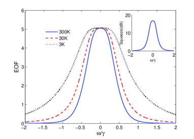
Figure 2: (Color online) EOF for different temperature. $|\alpha|$ is 1000, $\delta/2\pi=10$ MHz, $d=0.07\gamma$. The maxima squeezing is larger than $16$ dB when $T=300$ K.

We now estimate the bath noise influence in experimentally accessible conditions Schliesser et al. (2008). The cavity resonant frequency $\omega_{p}=2\pi\times 300$ THz. The oscillator frequency $\omega_{m}=2\pi\times 73.5$ MHz. The mechanical Q factor is about $30~{}000$. The cavity and oscillator modes decay rates are $\gamma=2\pi\times 3.2$ MHz and $\gamma_{m}=\omega_{m}/Q$, respectively. The cavity radius is $R=38$ $\mu$m. The dimensionless coupling parameter is $\eta\simeq 10^{-4}$. We find if $0<d\ll\gamma$, the thermal noise does not decrease the maximum entanglement with strong enough input power. This is because we adiabatically eliminate the mechanical mode and suppress the effects of thermal noise. As show in Fig. 2, the temperature change does not change the maximum entanglement with proper driving and detuning. But the higher the temperature, the less the entanglement spectrum width. The embeded figure shows that the maximum squeezing could be larger than $16$ dB at room temperature.

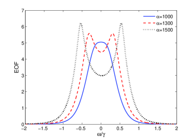
Figure 3: (Color online) EOF for different cavity mode amplitude $\alpha$. Here we adopt $\delta/2\pi=10$ MHz, $T=300$ K, $\gamma_{p}/2\pi=3.2$MHz, and $d=0.07\gamma$.

.

As shown in Fig. 3, the bigger the cavity mode amplitude $\alpha$, the larger the output entanglement. Because $\alpha_{j}\simeq\Omega_{j}/\sqrt{\gamma^{2}+4\Delta_{j}^{2}}$, the output entanglement is proportional to driving amplitude. But the peak of entanglement is splitted into two symmetric peaks when driving is very strong. The splitting distance is proportional to driving power. Increasing driving power can decrease the entanglement too. This is because adiabatical elimination condition $\omega\ll\delta$ are not valid around peaks for very strong driving. So the driving power should be neither too big nor too small. For the specific $\alpha$ and $\delta$, we find there is an optimum $d$ which makes entanglement maximum and the entanglement peaks appear near $\omega=0$. The optimum $d$ is $d_{o}=\sqrt{(\eta^{2}\omega^{2}\alpha^{2}/\delta)^{2}+\gamma^{2}/4}-(\eta\omega\alpha)^{2}/\delta$, corresponding to squeezing $S_{o}=-10\log_{10}(4d_{o}^{2}/\gamma^{2})$ and entanglement which is obtained from Eq. (12) with $n-kx=4(d_{o}/\gamma)^{2}$. It is obvious that the higher the input power, the smaller the optimum $d$. In the mean time, we find that decreasing the mechanical $Q$ factor nearly does not change the entanglement spectrum if $d$ is around its optimum value and the condition $\omega_{m}/Q\ll\delta$ is fulfilled. Leaving other parameters unchanged, $Q$ could be as low as $300$. Considering the difficulty of increasing the mechanical oscillator $Q$, the above finding makes our scheme more practical.

We also test the stability of our scheme. As shown in Fig. 4, the optimum $d$ is around $0.07\gamma$ if $\alpha=1000$, $\delta/2\pi=10$ MHz. To maintain such high entanglement, we need to precisely control the $d$ down to $0.02\gamma\sim 2\pi\times 60$ kHz. $d$ is defined as $d=-(\Delta_{1}^{\prime}+\Delta_{2}^{\prime})/2=-(\Delta_{1}+\Delta_{2})/2-4\eta^{2}\omega_{m}|\alpha|^{2}$. The higher entanglement is needed, the more precise detuning and driving power is required at the same time. To maintain the entanglement as high as Fig. 4, the laser spectrum width should be less than $60$ kHz and the driving power fluctuation should be less than $1\%$. The lower entanglement between two beams is needed to maintain, the larger the optimum $d$ is. Therefore higher fluctuations of detuning and driving power are allowed.

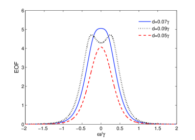
Figure 4: (Color online) EOF for different $d$. Here we adopt $\omega_{m}/2\pi=73.5$ MHz, $T=300$K, $\gamma_{m}=\omega_{m}/30~{}000$, $\gamma/2\pi=3.2$ MHz, and $|\alpha|=1000$.

.

Before conclusion, we briefly discuss the approximations we used. Our scheme needs the steady states existing, which requires $\langle a_{j}^{\dagger}a_{j}\rangle\ll|\alpha|^{2}$. During numerical calculation, $\langle a^{\dagger}a\rangle$ is in the order of $10^{3}$, which is much less than $|\alpha|^{2}\sim 10^{6}$. The other two approximations are rotating wave approximation $\omega_{m}\gg\delta,d,\gamma,\gamma_{m}$ and adiabatical elimination $\delta\gg\omega,\gamma_{m}$, which can be fulfilled independently. For $\alpha\sim 10^{3}$, the driving amplitude $\Omega$ is in the order of $10^{11}$ Hz, which is much lower than the distance between adjacent cavity modes $\Delta\omega=c/(Rn_{0})\sim 5\times 10^{12}$ Hz, where $c$ is the light speed in a vacuum, $n_{0}$ the refractive index of silica. Therefore the approximation that one laser only drives one cavity mode is valid. Laser power is needed in the order of $10$ mW, which is available in the laboratory.

In conclusion, we have proposed a scheme to generate EPR lights in an optomechanical system. Two sideband modes, which couple with the mechanical mode, are driven by lasers. After adiabatically eliminating the the mechanical mode, we find that the output sideband modes are highly entangled. The higher power of the driving laser, the larger entanglement of the output light. To maintain the entanglement, we need to precisely control the driving power and laser frequency at the same time. With proper parameters, the entanglement is insensitive to the thermal noise and mechanical $Q$ factor. We test the scheme by experimental available parameters. Though in this paper we fucus on WGM cavity systems, our scheme can be realized in other optomechanical systems, as long as the mechanical mode frequency is much larger than the cavity decay rate.

We thank Lu-ming Duan for helpful discussions. We thank Yun-feng Xiao and Qing Ai for valuable comments on the paper. ZY was supported by the Government of China through CSC (Contact No.2007102530).

References

• Braunstein and Loock (2005) S. L. Braunstein and P. V. Loock, Rev. Mod. Phys. 77, 513 (2005).
• Ou et al. (1992) Z. Y. Ou, S. F. Pereira, H. J. Kimble, and K. C. Peng, Phys. Rev. Lett. 68, 3663 (1992).
• Silberhorn et al. (2001) C. Silberhorn, P. K. Lam, O. Weiß, F. König, N. Korolkova, and G. Leuchs, Phys. Rev. Lett. 86, 4267 (2001).
• Hilico and et al. (1992) L. Hilico and et al., Appl. Phys. B 55, 202 (1992).
• Mancini and Tombesi (1994) S. Mancini and P. Tombesi, Phys. Rev. A 49, 4055 (1994).
• Fabre et al. (1994) C. Fabre, M. Pinard, S. Bourzeix, A. Heidmann, E. Giacobino, and S. Reynaud, Phys. Rev. A 49, 1337 (1994).
• Giovannetti et al. (2001) V. Giovannetti, S. Mancini, and P. Tombesi, Europhys. Lett. 54, 559 (2001).
• Mancini and Gatti (2001) S. Mancini and A. Gatti, J. Opt. B: Quantum Semiclass. Opt. 3, S66 (2001).
• Pirandola et al. (2003) S. Pirandola, s. Mancini, D. Vitali, and P. Tombesi, J. Opt. B: Quantum Semiclass. Opt. 5, S523 (2003).
• Genes et al. (2008) C. Genes, A. Mari, P. Tombesi, and D. Vitali, Phys. Rev. A 78, 032316 (2008).
• Wipf et al. (2008) C. Wipf, T. Corbitt, Y. Chen, and N. Mavalvala, New J. Phys. 10, 095017 (2008).
• Regal1 et al. (2008) C. A. Regal1, J. D. Teufel, and K. W. Lehnert, Nat Phys 4, 555 (2008).
• Schliesser et al. (2008) A. Schliesser, R. Riviere, G. Anetsberger, O. Arcizet, and T. J. Kippenberg, Nat Phys 4, 415 (2008).
• Schliesser et al. (2008) A. Schliesser, G. Anetsberger, R. Rivière, O. Arcizet, and T. J. Kippenberg, New J. Phys. 10, 095015 (2008).
• Giedke et al. (2003) G. Giedke, M. M. Wolf, O. Krüger, R. F. Werner, and J. I. Cirac, Phys. Rev. Lett. 91, 107901 (2003).
• Spillane et al. (2003) S. M. Spillane, T. J. Kippenberg, O. J. Painter, and K. J. Vahala, Phys. Rev. Lett. 91, 043902 (2003).
• Wilson-Rae et al. (2007) I. Wilson-Rae, N. Nooshi, W. Zwerger, and T. J. Kippenberg, Phys. Rev. Lett. 99, 093901 (2007).
• Marquardt et al. (2007) F. Marquardt, J. P. Chen, A. A. Clerk, and S. M. Girvin, Phys. Rev. Lett. 99, 093902 (2007).
• Dayan et al. (2008) B. Dayan, A. S. Parkins, T. Aoki, E. P. Ostby, K. J. Vahala, and H. J. Kimble, Science 319, 1062 (2008).
• Srinivasan and Painter (2007) K. Srinivasan and O. Painter, Phys. Rev. A 75, 023814 (2007).
• Kippenberg and Vahala (2007) T. J. Kippenberg and K. J. Vahala, Optics Express 15, 17172 (2007).
• Walls and Milburn (1994) D. F. Walls and G. J. Milburn, Quantum Optics (Springer-Verlag, Berlin, 1994).