Isospin mixing effects in low-energy $\bar{K}N-\pi\Sigma$ interaction

Abstract

New strong coupled-channel $\bar{K}N-\pi\Sigma$ potential, reproducing all existing experimental data and suitable for using in an accurate few-body calculations, is constructed. Isospin breaking effects of direct inclusion of the Coulomb interaction and using of physical masses in calculations are investigated. The $1s$ level shift and width of kaonic hydrogen, consistent with the scattering data, was obtained and the corresponding exact strong $K^{-}p$ scattering length was calculated. One- and two-pole form of $\Lambda(1405)$ resonance was considered.

I Introduction

Kaonic atoms and, especially, possibility of formation of kaonic nuclear clusters attracted large interest recently. For investigation of these systems it is necessary to know the basic $\bar{K}N$ interaction, which is strongly connected with $\pi\Sigma$ and other channels.

Different theoretical models were used for constructing antikaon-nucleon interaction. All these models can be separated in two groups: “stand-alone” potentials only fitting two-body data and potentials to be used in future (few- or many-body) calculations.

To the first group belong very popular in our days potentials based on chiral Lagrangian. The method consists of constructing a potential which gives amplitudes equivalent to those derived from an effective chiral lagrangian. Such potentials have many channels, including energetically closed near $\bar{K}N$ threshold ones. The most recent example is a model constructed in Borasoy_KN ; Borasoy_aKp . It is good in reproducing the antikaon-nucleon experimental data, however, due to its unhandiness the potential cannot be used in few- or many-body calculations.

On the other hand, effective potentials used in approximate few-body calculations are too simple for proper describing of all properties of $\bar{K}N$ system. In most cases a one-channel (effective) optical potential is used. For example, $\bar{K}N$ potential, used in ay for calculating of deeply-bound kaonic nuclear states, is an energy-independent optical potential. It was constructed in such a way that it corresponds to the elastic part of a coupled-channel phenomenological $\bar{K}N-\pi\Sigma-\pi\Lambda$ potential. However, already the coupled-channel potential is too simple. One more example is a recent work 2bWeise , where a potential for further use in a few-body calculation was derived. It is once more an effective energy-dependent optical potential by construction: it reproduces the elastic part of an effective chiral coupled-channel model.

Two-body optical potential could be equivalent to the original coupled-channel ones. For separable potentials it is possible to construct exact optical potential, but even an exact optical potential properly describes only the elastic part of the whole system. Moreover, introducing such “good” effective optical potential into $N>2$ equations does not guarantee proper description of all inelastic effects taking place in a few- or many-body system.

The inelastic effects are especially important for the antikaon-nuclear systems, because $\bar{K}N$ interaction is strongly coupled to the $\pi\Sigma$ channel through $\Lambda(1405)$ resonance. However, the nature of the resonance is a separate question. A usual assumption is that $\Lambda(1405)$ is a resonance in $\pi\Sigma$ and a quasi-bound state in $\bar{K}N$ channel. There is also an assumption suggested by a chiral model, that the bump, which is usually understood as $\Lambda(1405)$ resonance, is an effect of two poles (see e.g. 2L1405 , MagasOset ). Some challenge to the two pole model was put by the recent experiment at COSY-Jülich Zychor , but a subsequent theoretical paper geng seems to reproduce the experiment on the basis of the two pole model.

Other sources of experimental data about $\bar{K}N$ interaction are also non-precise, old or controversial. The data on cross-sections of elastic and inelastic scattering with $K^{-}p$ in the initial state are rather old with rather large errors, while threshold branching ratios of $K^{-}p$ scattering were measured more accurately.

Another source of knowledge about $\bar{K}N$ is kaonic hydrogen atom. Several experiments were performed for measuring $1s$ level shift caused by strong $\bar{K}N$ interaction. The two recent ones are KEK KEK1s and DEAR DEAR1s results. More recent DEAR value of $1s$ level shift and width significantly differs from the older KEK result, it has smaller errors, but is inconsistent with the scattering $K^{-}p$ data as was shown in Borasoy_KN ; Borasoy_aKp .

Moreover, there is a problem common for both experimental papers: they present a $K^{-}p$ scattering length following from the measurements as an “experimental value”. However, $a_{K^{-}p}$ values in KEK1s and DEAR1s were obtained using Deser-Trueman (DT) formula Deser , while in many papers (among them in Revai for several one-channel model potentials) it was shown, that the approximate formula has poor accuracy, in particular for the $\bar{K}N$ interaction. There are several papers, introducing different corrections to DT, nowadays the most popular is a formula from Ruzecky . Undoubtedly, the corrected formula Ruzecky has the same advantage as original DT Deser one: it is a model-independent relation between scattering length and atomic level shift and width. Its accuracy can be checked within a potential model where exact calculations are feasible.

Since the measured value is the $1s$ level shift and width (and not the $K^{-}p$ scattering length) we decided to construct a phenomenological coupled-channel potential, reproducing kaonic hydrogen’s level shift and width without intermediate reference to $a_{K^{-}p}$. It is clear that for reproducing the level shift of kaonic hydrogen it is necessary to include Coulomb interaction into equations directly, which beaks isospin symmetry. As far as we know, the only attempt to do the same was performed in Cieply . The authors used their own method for calculating kaonic atomic state with separable chiral-based strong part of the potential and tried to reproduce DEAR data. However, the resulting potential Cieply provides too large width $\Gamma$ of $1s$ kaonic hydrogen level in comparison with DEAR values, moreover, there are problems with reproducing $\Lambda(1405)$ resonance. The first version of our $\bar{K}N-\pi\Sigma$ potential reproducing $1s$ level shift instead of $K^{-}p$ scattering length with direct inclusion of the Coulomb interaction, and the corresponding three-body $\bar{K}NN-\pi\Sigma N$ calculation using the obtained potential was presented in Pisa_proc_my .

There is one more approximation which is widely used in theoretical models, namely, neglecting the mass difference in iso-multiplets. However, the difference of masses between proton and neutron and $K^{-}$ and $\bar{K}^{0}$ is a physical fact. Besides, the effect of taking the mass difference into account is especially important in the near-threshold $\bar{K}N$ region. Using the physical masses in the calculations is one more isospin symmetry breaking effect, taken into account in the paper.

Thus, our aim is to construct phenomenological coupled-channel $\bar{K}N-\pi\Sigma$ potential, which within the limits of the possible simultaneously reproduce all experimental data: the level shift and width of kaonic hydrogen $1s$ level (KEK or DEAR values), $K^{-}p$ threshold branching ratios, elastic and inelastic $K^{-}p$ scattering, and $\Lambda(1405)$ resonance in one- or two-pole form. We directly include such isospin breaking effects as Coulomb interaction and using the physical masses of particles in the calculations. The corresponding $T$-matrix should be suitable for using in an accurate few-body (for example, three-body coupled-channel Faddeev) calculation.

II Formulation of the problem

Our non-relativistic Hamiltonian has the form

$$H=H^{0}+V^{c}+V^{s}$$ (1)

with $H^{0}$ being the kinetic energy plus the threshold energy of particle pairs, $V^{c}$ and $V^{s}$ denote their Coulomb and strong interaction, respectively. The transition matrix for the problem defined by this Hamiltonian can be written as

$$T_{ba}=T_{ba}^{c}+T_{ba}^{sc},$$ (2)

where $T_{ba}^{c}$ is the pure Coulomb transition matrix, while $T_{ba}^{sc}$ is the so called Coulomb-modified strong transition matrix, defined as

$$T_{ba}^{sc}=\langle\Phi_{b}^{c(-)}|V^{s}|\Psi_{a}^{(+)}\rangle.$$ (3)

Here $|\Phi_{b}^{c(\pm)}\rangle$ is a Coulomb scattering state labeled by the final state index $b$, while $|\Psi_{a}^{(+)}\rangle$ denotes the total scattering state, corresponding to the initial state labeled $a$ and satisfying the Lippmann-Schwinger equation

$$|\Psi_{a}^{(+)}\rangle=|\Phi_{a}^{c(+)}\rangle+G^{c}(E+i\varepsilon)V^{s}|\Psi_{a}^{(+)}\rangle$$ (4)

with the Coulomb Green’s function

$$G^{c}(z)=(z-H^{0}-V^{c})^{-1}\ .$$ (5)

For a separable strong potential taken as $V^{s}=|g\rangle\lambda\langle g|$ the $T_{ba}^{sc}$ matrix (3) has a form

$$T_{ba}^{sc}=\langle\Phi_{b}^{c(-)}|g\rangle(\lambda^{-1}-\langle g|G^{c}(E+i\varepsilon)|g\rangle)^{-1}\langle g|\Phi_{a}^{c(+)}\rangle\ .$$ (6)

For sufficiently simple form-factors $|g\rangle$ the matrix elements of the Coulomb Green’s function $\langle g|G^{c}(E+i\varepsilon)|g\rangle$ together with the overlaps $\langle g|\Phi_{a}^{c(\pm)}\rangle$ in Eq.(6) can be calculated analytically (see e.g. gGg_Coul1 ; gGg_Coul2 ; gGg_Coul3 ). The poles of the total $T_{ba}(z)$ matrix in this case are determined by the equation

$$\lambda^{-1}-\langle g|G^{c}(z)|g\rangle=0\ ,$$ (7)

since it can be shown, that the poles of the pure Coulomb $T_{ba}^{c}$ matrix are canceled out from Eq.(2).

The non-relativistic description of transitions allowing for change of particle composition is achieved by enlarging the Hilbert-space by adding to it a discrete “particle composition” index. In this case the operators and wave functions become matrices and vectors with respect to this index. The details of the matrix formulation of Eqs.(3)–(7) are described in the Appendix.

III Details of the calculation and the input

In momentum representation the strong interaction matrix (A.16) can be written as:

$$V^{s}_{\mathbb{I}_{i},\mathbb{I}_{j}}(k_{\mathbb{\,I}_{i}},k_{\mathbb{\,I}_{j}})=\delta_{I(\mathbb{I}_{i}),I(\mathbb{I}_{j})}\,g_{\mathbb{I}_{i}}(k_{\,\mathbb{I}_{i}})\lambda_{\mathbb{I}_{i},\mathbb{I}_{j}}\,g_{\mathbb{I}_{j}}(k_{\,\mathbb{I}_{j}})$$ (8)

with $g_{\mathbb{I}_{i}}(k_{\,\mathbb{I}_{i}})=\langle\vec{k}_{\,\mathbb{I}_{i}}|g_{\mathbb{I}_{i}}\rangle$, $\vec{k}_{\,\mathbb{I}_{i}}$ being the relative momentum of the particles in $\mathbb{I}_{i}$. We use the $\hbar=c=1$ system of units, our plane waves are normalized as $\langle\vec{k}|\vec{k}^{\prime}\rangle=\delta(\vec{k}-\vec{k}^{\prime})$. In this case the scattering amplitude $f_{ba}$ is connected with $T_{ba}$ by:

$$f_{ba}=-(2\pi)^{2}\ \sqrt{\mu_{a}\mu_{b}}\ T_{ba},$$ (9)

where $\mu_{a}$ ($\mu_{b}$) is the reduced mass of the particles in the initial (final) state.

We tried to reproduce simultaneously the following experimental data (A–D).

III.1 $\Lambda(1405)$ resonance

Mass $M_{\Lambda}$ and width $\Gamma_{\Lambda}$ of the $\Lambda(1405)$ resonance according to the Particle Data Group PDG are:

$$M_{\Lambda}^{\,\rm PDG}=1406.5\pm 4.0\;{\rm MeV},\quad\Gamma_{\Lambda}^{\,\rm PDG}=50.0\pm 2.0\;{\rm MeV}.$$ (10)

Unlike to PDG, our $\Lambda(1405)$ is not a clear $I=0$ state, but a mixture of $I=0$ and $I=1$ states. Having in mind existing assumptions, we used two versions of $\Lambda(1405)$’s “nature”: one- and two-pole ones. For the one-pole form of $\Lambda(1405)$ we used Yamaguchi form-factors:

$$g_{\mathbb{\,I}_{i}}^{1pole}(k_{\mathbb{\,I}_{i}})=\frac{1}{(k_{\mathbb{\,I}_{i}})^{2}+(\beta_{\mathbb{\,I}_{i}})^{2}},\quad i=1,\dots,5.$$ (11)

We assumed $\Lambda(1405)$ as a resonance in $\pi\Sigma$ and a quasi-bound state in $\bar{K}N$ channel. So, calculation of (53) was done at physical sheet for $\bar{K}N$ and non-physical sheet for $\pi\Sigma$ channel.

For two-pole case we assumed that there are two resonances in $\pi\Sigma$ channel. One of them, as before, originates from a bound state in $\bar{K}N$ channel, the other one from a resonance in $\pi\Sigma$ channel (with $\bar{K}N-\pi\Sigma$ coupling switched off). It is known that in a one-channel case a one-term separable potential with Yamaguchi form-factors (11) and real strength parameters can not describe a resonance. So, in order to have a resonance in the uncoupled $\pi\Sigma$ channel, for two-pole $\Lambda(1405)$ case we used $\pi\Sigma$ form-factors in the following form:

$$g_{\mathbb{\,I}_{i}}^{2pole}(k_{\mathbb{\,I}_{i}})=\frac{1}{(k_{\mathbb{\,I}_{i}})^{2}+(\beta_{\mathbb{\,I}_{i}})^{2}}\,+\,\frac{s\,(\beta_{\mathbb{\,I}_{i}})^{2}}{[(k_{\mathbb{\,I}_{i}})^{2}+(\beta_{\mathbb{\,I}_{i}})^{2}]^{2}},\quad i=3,4,5.$$ (12)

By this for the two-pole case we introduced one more parameter $s$. For the $\bar{K}N$ channel here we used Yamaguchi form-factors:

$$g_{\mathbb{\,I}_{i}}^{2pole}(k_{\mathbb{\,I}_{i}})=\frac{1}{(k_{\mathbb{\,I}_{i}})^{2}+(\beta_{\mathbb{\,I}_{i}})^{2}},\quad i=1,2.$$ (13)

Both poles are once more situated at physical sheet for $\bar{K}N$ and non-physical sheet for $\pi\Sigma$ channel.

III.2 Kaonic hydrogen data

The $K^{-}p$ atomic $1s$ level shift $\Delta E_{1s}$ and width $\Gamma_{1s}$ measured in the KEK experiment KEK1s

$$\Delta E^{KEK}_{1s}=-323\pm 63\pm 11\;{\rm eV},\quad\Gamma^{KEK}_{1s}=407\pm 208\pm 100\;{\rm eV}$$ (14)

and in the DEAR collaboration experiment DEAR1s

$$\Delta E^{DEAR}_{1s}=-197\pm 37\pm 6\;{\rm eV},\quad\Gamma^{DEAR}_{1s}=249\pm 111\pm 30\;{\rm eV}$$ (15)

differs from each other. We tried to reproduce both these values within $1\sigma$ interval.

We would like to stress, that in our approach there is no intermediate reference to $K^{-}p$ scattering length when reproducing the level shift and the width. Of course, after finding a set of potential parameters we can calculate a strong scattering length, which exactly corresponds to the obtained $1s$ level shift $\Delta E_{1s}$ and width $\Gamma_{1s}$. Due to the isospin symmetry breaking the formula for the $a_{K^{-}p}$ differs from commonly used $\frac{1}{2}\,(a_{\bar{K}N,I=0}+a_{\bar{K}N,I=1})$, since our $T$-matrix has non-diagonal elements between $I=0$ and $I=1$ states.

We mention here, that energies of atomic (kaonic hydrogen $1s$ level) and nuclear (one- and two-pole $\Lambda(1405)$) states are obtained from the same system of equations (53). The second remark concerns the origin of the resonances. All our resonances are poles on the corresponding sheet of the complete problem. Since our formula (53) was obtained by solving dynamical equations, the resonances can be rightly called dynamically generated ones.

III.3 Scattering data

Elastic and inelastic total cross sections with $K^{-}p$ in the initial state were measured in Kp2exp ; Kp3exp ; Kp4exp ; Kp5exp ; Kp6exp (we did not take into consideration data from Kp1exp with huge error bars). It is interesting, that there are no comments about non-existence of the total elastic cross-sections (except Borasoy_KN and Borasoy_aKp ) due to the singularity of the pure Coulomb transition matrix $T_{ba}^{c}$ in (2), while the “total elastic” cross-sections are plotted by almost every author of $\bar{K}N$ interaction models. Having Coulomb interaction directly included into the calculations we could not ignore the problem. We defined “total elastic” $K^{-}p$ cross-section following the experimental works Kp1exp ; Kp2exp . Namely, the total cross-sections were obtained by integrating differential cross-sections in the region $-1\leq\cos{\theta}\leq 0.966$ instead of $-1\leq\cos{\theta}\leq 1$.

III.4 Threshold branching ratios

Three threshold branching ratios of $K^{-}p$ scattering were measured rather accurately gammaKp1 ; gammaKp2 . One of them is

$$\gamma=\frac{\Gamma(K^{-}p\to\pi^{+}\Sigma^{-})}{\Gamma(K^{-}p\to\pi^{-}\Sigma^{+})}=2.36\pm 0.04\,.$$ (16)

We oriented on the medium value

$$\gamma=2.36.$$ (17)

The other two ratios $R_{c}$ and $R_{n}$, containing $K^{-}p\to\pi^{0}\Lambda$ cross-sections,

$$R_{c} = \frac{\Gamma(K^{-}p\to\pi^{+}\Sigma^{-},\pi^{-}\Sigma^{+})}{\Gamma(K^{-}p\to\mbox{all inelastic channels})}=0.664\pm 0.011,$$ (18)

$$R_{n} = \frac{\Gamma(K^{-}p\to\pi^{0}\Lambda)}{\Gamma(K^{-}p\to\mbox{neutral states})}=0.189\pm 0.015,$$ (19)

could not be used in a straightway because we did not include $\pi^{0}\Lambda$ channel directly into our calculations. However, the effect of the channel was effectively taken into account by allowing $\lambda^{1}_{\bar{K}N,\bar{K}N}$ parameter to have non-zero imaginary part (it significantly improved the agreement with the experimental cross-sections). It is easy to find from the measured $K^{-}p$ threshold branching ratios $\gamma$, $R_{c}$, and $R_{n}$, that relevant weight of $\pi^{0}\Lambda$ channel at $K^{-}p$ threshold among all possible inelastic channels is approximately equal to $6\%$. So, the introduced imaginary part only slightly breaks unitarity in contrast to what happens when a one-channel complex $\bar{K}N$ potential is used, approximately accounting for the main inelastic $\pi\Sigma$ channel.

From existing $R_{c}$ and $R_{n}$ we constructed a new threshold branching ratio

$$R_{\pi\Sigma}=\frac{\Gamma(K^{-}p\to\pi^{+}\Sigma^{-})+\Gamma(K^{-}p\to\pi^{-}\Sigma^{+})}{\Gamma(K^{-}p\to\pi^{+}\Sigma^{-})+\Gamma(K^{-}p\to\pi^{-}\Sigma^{+})+\Gamma(K^{-}p\to\pi^{0}\Sigma^{0})}\,.$$ (20)

From definitions of $R_{c}$ and $R_{n}$ (18), (19) using experimental data we obtained for the $R_{\pi\Sigma}$ an “experimental” value

$$R_{\pi\Sigma}=\frac{R_{c}}{1-R_{n}\,(1-R_{c})}\,=\,0.709\pm 0.011\,.$$ (21)

We tried to reproduce the medium value

$$R_{\pi\Sigma}=0.709.$$ (22)

The formulae (52) and (53) allow us to find parameters $\lambda_{\mathbb{I}_{i},\mathbb{I}_{j}}$, $\beta_{\mathbb{I}_{i}}$ (and $s$) of our potentials in both one-pole and two-pole cases, which reproduce these experimental quantities. All our parameters, except $\lambda^{1}_{\bar{K}N,\bar{K}N}$, are real.

IV Results and discussion

We started the calculations with inclusion of the Coulomb interaction and using physical masses in both $\bar{K}N$ and $\pi\Sigma$ channels. However, it turned out, that the effects are small for the $\pi\Sigma$ subsystem compared to those for the antikaon-nucleon channel. It is understandable, since we are interested in the energy region near $\bar{K}N$ threshold, where the mass difference between $K^{-}$ and $\bar{K}^{0}$, $p$ and $n$ should manifest itself, at least, by the existence of two close thresholds for $K^{-}p$ and $\bar{K}^{0}n$ in contrast to the one threshold for $\bar{K}N$. Due to this we kept the Coulomb potential in $K^{-}p$ subsystem and physical masses in $\bar{K}N_{I=0},\bar{K}N_{I=1}$ ($K^{-}p,\bar{K}^{0}n$) channels, while in $\pi\Sigma$ channels we used isospin averaged masses without the Coulomb interaction.

In the case of averaged masses without Coulomb in $\pi\Sigma$ the $\pi\Sigma_{I=2}$ ($\mathbb{I}_{5}$) channel is dynamically decoupled from the other four channels. So, we can work in particle space of four dimensions, corresponding to $\bar{K}N_{I=0}$, $\bar{K}N_{I=1}$ (or $K^{-}p,\bar{K}^{0}n$), $\pi\Sigma_{I=0}$, and $\pi\Sigma_{I=1}$ channels.

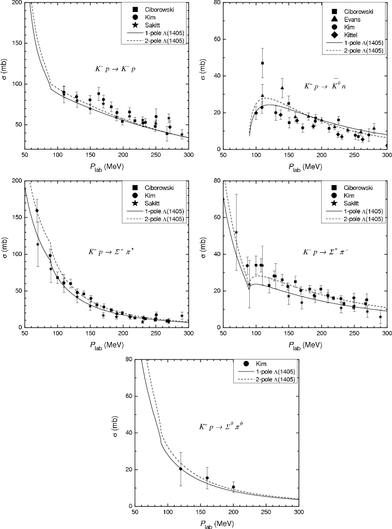
Figure 1: Comparison of the obtained theoretical cross-sections (lines) with experimental data Kp2exp ; Kp3exp ; Kp4exp ; Kp5exp ; Kp6exp (points). Solid lines: calculation with 1-pole $\Lambda(1405)$ resonance, dashed lines: calculation with 2-pole $\Lambda(1405)$ resonance.

We succeeded in obtaining parameters of the potentials with one- and two-pole $\Lambda(1405)$ structure. The best set of the obtained parameters for the one-pole $\Lambda(1405)$ is:

$$\begin{tabular}[]{c}$\beta^{1pole}_{\bar{K}N}=3.4{\rm\;fm}^{-1}$\\ $\beta^{1pole}_{\pi\Sigma}=1.9{\rm\;fm}^{-1}$\end{tabular}\qquad\underline{\underline{\Lambda}}^{1pole}(\mathbb{I})=\left(\begin{tabular}[]{cccc}$-1.31$&$0$&$0.62$&$0$\\ $0$&$1.76-i0.24$&$0$&$1.90$\\ $0.62$&$0$&$0.18$&$0$\\ $0$&$1.90$&$0$&$1.24$\end{tabular}\right)$$ (23)

for the two-pole $\Lambda(1405)$ it is:

$$\begin{tabular}[]{c}$\beta^{2pole}_{\bar{K}N}=3.2{\rm\;fm}^{-1}$\\ $\beta^{2pole}_{\pi\Sigma}=1.0{\rm\;fm}^{-1}$\\ $s=-0.87$\end{tabular}\qquad\underline{\underline{\Lambda}}^{2pole}(\mathbb{I})=\left(\begin{tabular}[]{cccc}$-1.06$&$0$&$0.40$&$0$\\ $0$&$0.97-i0.11$&$0$&$1.13$\\ $0.40$&$0$&$-0.01$&$0$\\ $0$&$1.13$&$0$&$0.61$\end{tabular}\right)\,.$$ (24)

Here we assumed isospin-independence of the range parameters:

$$\beta_{\mathbb{\,I}_{1}}=\beta_{\mathbb{\,I}_{2}}\equiv\beta_{\bar{K}N},$$ (25)

$$\beta_{\mathbb{\,I}_{3}}=\beta_{\mathbb{\,I}_{4}}\equiv\beta_{\pi\Sigma}.$$ (26)

Our results for the cross-sections with best set of the obtained parameters with one-pole and two-pole $\Lambda(1405)$ are presented in Fig. 1: the elastic $K^{-}p\to K^{-}p$ cross-section and inelastic $K^{-}p\to\bar{K}^{0}n$, $K^{-}p\to\pi^{+}\Sigma^{-}$, $K^{-}p\to\pi^{-}\Sigma^{+}$, and $K^{-}p\to\pi^{0}\Sigma^{0}$ cross-sections are compared with existing experimental data Kp2exp ; Kp3exp ; Kp4exp ; Kp5exp ; Kp6exp . It is seen, that both versions of the potential are equally good in describing the experimental data within the experimental errors. Due to this fact, unfortunately, it is not possible to give preference to one of the $\Lambda(1405)$ versions.

Other physical characteristics of the obtained 1-pole and 2-pole potentials are shown in Table 1: pole positions $z_{1}$ and $z_{2}$ (obviously, $z_{2}$ exists in 2-pole variant of the potential only), $1s$ kaonic hydrogen level shift $\Delta E_{1s}$ and width $\Gamma_{1s}$. Threshold branching ratios $\gamma$ (17) and $R_{\pi\Sigma}$ (22) are reproduced exactly in both cases. Having complete set of potential parameters it is possible to calculate the strong $K^{-}p$ scattering length corresponding to the given $\Delta E_{1s}$ and $\Gamma_{1s}$ exactly. The $a_{K^{-}p}$ for both potentials are also shown in the Table 1.

Table 1: Physical characteristics of the obtained 1-pole and 2-pole potentials: pole positions $z_{1}$ and $z_{2}$, level shift $\Delta E_{1s}$ and width $\Gamma_{1s}$ of kaonic hydrogen, and corresponding exact strong scattering length $a_{K^{-}p}$. Threshold branching ratios (17) and (22) are reproduced exactly.

	1-pole $\Lambda(1405)$	2-pole $\Lambda(1405)$
$z_{1}$ (MeV)	$1409-i32$	$1412-i32$
$z_{2}$ (MeV)	$-$	$1380-i105$
$\Delta E_{1s}$ (eV)	$-396$	$-407$
$\Gamma_{1s}$ (eV)	$370$	$476$
$a_{K^{-}p}$ (fm)	$-1.07+i0.59$	$-1.08+i0.76$

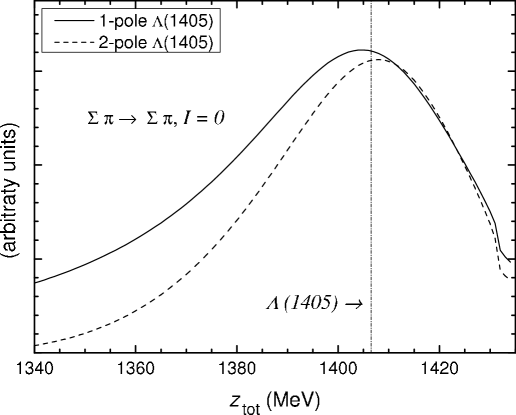
Figure 2: Manifestation of $\Lambda(1405)$ resonance in $I=0$ $\pi\Sigma\to\pi\Sigma$ cross-section, solid line: calculation with 1-pole $\Lambda(1405)$, dashed line: calculation with 2-pole $\Lambda(1405)$ resonance. The vertical line marks the medium PDG mass $M^{PDG}_{\Lambda}=1406.5$ MeV of the resonance PDG .

The first pole positions $z_{1}$ for both versions of the potential have close real parts and the same imaginary ones, however, all three numbers differ from the PDG data for mass and width of $\Lambda(1405)$ resonance (10). The characteristics of the two poles $z_{1}$ and $z_{2}$ in the 2-pole $\Lambda(1405)$ version are the same as in MagasOset : one of them has less mass and larger width, while the other is heavier with narrower width. However, the positions of $z_{1}$ and $z_{2}$ differ from those in MagasOset .

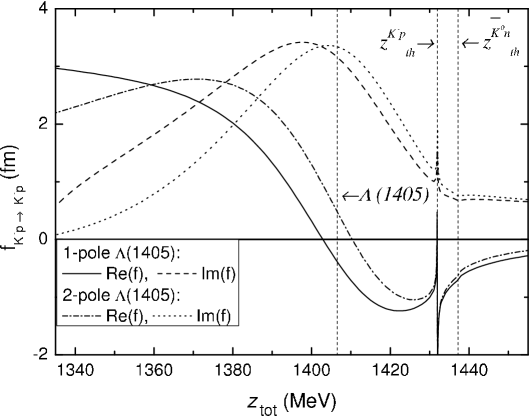
Figure 3: Manifestation of $\Lambda(1405)$ resonance in $K^{-}p\to K^{-}p$ amplitude below the threshold for both versions of the potential. One-pole $\Lambda(1405)$: real (solid line) and imaginary part (dashed line) of $f_{K^{-}p\to K^{-}p}$. Two-pole $\Lambda(1405)$: real (dash-dotted line) and imaginary part (dotted line) of the amplitude. The vertical lines marks the medium PDG mass $M^{PDG}_{\Lambda}=1406.5$ MeV of the resonance PDG , $K^{-}p$ and $\bar{K}^{0}n$ thresholds.

It is not absolutely clear, how to relate the obtained potentials to the shape of the $\Lambda(1405)$ resonance. The experimental shape of the resonance is deduced from missing mass experiments since direct $\pi\Sigma$ data are not available. However, their relation to the pole structure of the two-body $T$-matrix is not trivial and needs further investigation. An example of the interpretation ambiguity is shown in Fig. 2, where we demonstrate the manifestation of $\Lambda(1405)$ in a calculated isospin-zero elastic $\pi\Sigma$ cross-section. It can be seen, that the maxima of the resonances for the two versions of the potential lay on opposite sides of the medium PDG value $M^{PDG}_{\Lambda}=1406.5$ MeV PDG , while both Re$(z_{1})$ are larger, than $1406.5$ MeV (see Table 1).

Another example is given in Fig. 3, where real and imaginary parts of the elastic $K^{-}p$ amplitude for the two versions of the potential are depicted. At the the resonance positions real parts of $f_{K^{-}p\to K^{-}p}$ have zeros (situated at different, in respect to the medium PDG value, sides), while imaginary parts have their maxima (at slightly lower energies). The Coulomb singularities are seen almost at the $K^{-}p$ threshold.

We plotted also the obtained parameters of kaonic hydrogen ($\Gamma_{1s},|\Delta E_{1s}|$), shown in Table 1, together with the experimental $1\sigma$ regions of KEK and DEAR results, see Fig. 4. It is seen, that obtained $\Delta E$ for the 1-pole version is situated inside the KEK region, while for the 2-pole variant it is slightly outside. Both values are close to each other, they definitely prefer the largest values of KEK $|\Delta E|$. All our attempts to move the shift values to the DEAR region led to drastic worsening of the agreement with the experimental cross-sections. From this fact we do the same conclusion as did authors of Borasoy_aKp : the DEAR data on kaonic hydrogen measurements are inconsistent with the existing scattering data.

As for the widths, both are situated inside KEK $1\sigma$ limits, while the 1-pole potential gives $\Gamma_{1s}$ also inside DEAR, closely to its highest possible value. The important fact is that the obtained theoretical values of $\Gamma_{1s}$ for the two versions of potentials have rather large difference. But, unfortunately, the accuracy of KEK results does not allow to make a unique selection between them.

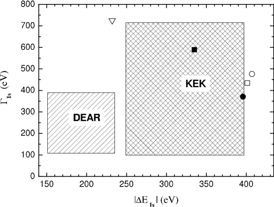
Figure 4: DEAR and KEK $1\sigma$ confidence region of kaonic hydrogen $1s$ level shift $|\Delta E|$ (absolute value) and width $\Gamma$. The obtained theoretical results for the one-pole (solid circle) and two-pole (empty circle) variants of the potential are shown. The results of other theoretical models are also depicted: Borasoy_KN  (solid square), Borasoy_aKp  (empty sqare), and Cieply  (empty triangle).

For comparison we plotted also the results of other theoretical models: Borasoy_KN , Borasoy_aKp , and Cieply . The first two ($\Gamma_{1s},|\Delta E_{1s}|$) values were obtained from the $K^{-}p$ scattering lengths using corrected DT formula Ruzecky , while the last one was calculated directly. The chiral potential Borasoy_aKp , aiming to reproduce mainly the $K^{-}p$ scattering data, have the result (corresponding to the best $a_{K^{-}p}$ value in the full approach) impressively close to our, though the correctness of it is limited by the corrected DT formula accuracy. The previous potential of the same authors (version “u”) have different ($\Gamma_{1s},|\Delta E_{1s}|$) value, however, is also situated inside $1\sigma$ KEK region. The result of Cieply is far from all other theoretical values and outside both experimental regions. The reason could be their attempt to fit DEAR values simultaneously with the scattering data, which turned out to be unsuccessful. It is an additional demonstration of inconsistency of the DEAR results with the existing scattering data.

We see that both versions of our potential reproduce experimental cross-sections equally well, by construction they exactly reproduce threshold branching ratios $\gamma$ and $R_{\pi\Sigma}$. The obtained values of the kaonic hydrogen level shift $\Delta E_{1s}$ in both versions of $\Lambda(1405)$ resonance are close to each other. However, there is rather large, more than $100$ eV, difference between the $K^{-}p$ widths $\Gamma_{1s}$. Having in mind a forthcoming experiment SIDDHARTA SIDDHARTA , we hope, that the new experimental value will be close to one of our numbers allowing to make a conclusion about the structure of $\Lambda(1405)$ resonance.

Table 2: Isospin conserving $a^{cons}$ (fm) and non-conserving $a^{nonc}$ (fm) constituents of the total $a$ (fm) $K^{-}p$ scattering length for one-pole and two-pole versions of the potential.

	1-pole $\Lambda(1405)$	2-pole $\Lambda(1405)$
$a^{cons}_{K^{-}p}$	$-1.0561+i0.6977$	$-0.9949+i0.8648$
$a^{nonc}_{K^{-}p}$	$0.0139+i0.1077$	$0.0851+i0.1048$
$a_{K^{-}p}$	$-1.07+i0.59$	$-1.08+i0.76$

The combined effect of the exact inclusion of the Coulomb interaction and using physical masses of the particles can be illustrated by showing the isospin conserving and non-conserving parts of the $K^{-}p$ scattering length, see Table 2. The constituents are defined as

$$a_{K^{-}p}^{cons}\equiv\frac{1}{2}\,\left(a^{00}_{\bar{K}N}+a^{11}_{\bar{K}N}\right),$$ (27)

$$a_{K^{-}p}^{nonc}\equiv a^{01}_{\bar{K}N}=a^{10}_{\bar{K}N},$$ (28)

where $a^{II^{\prime}}_{\bar{K}N}$ denotes the elastic strong (Coulomb is switched off) $\bar{K}N$ on-shell amplitude with initial (final) pair isospin I’ (I) at the $K^{-}p$ threshold. The total scattering length, also shown in Table 2, is

$$a_{K^{-}p}=a_{K^{-}p}^{cons}-a_{K^{-}p}^{nonc}\,.$$ (29)

It is seen, that real parts of non-conserving scattering lengths change the final results only slightly, especially in the one-pole case, where $a_{K^{-}p}^{nonc}$ is $1\%$ of $a_{K^{-}p}$ (it is $8\%$ for the two-pole variant). In contrast, the imaginary parts change isospin conserving scattering lengths essentially, the share of isospin non-conserving part is $18\%$ for the one-pole and $14\%$ for the two-pole case. Thus, isospin breaking effects, taken into account in our calculations, are important, especially for the strong $K^{-}p$ scattering length.

Table 3: Kaonic hydrogen $1s$ level shift $\Delta E$ (eV) and width $\Gamma$ (eV), corresponding to the obtained scattering length: exact (this work), derived from Deser-Trueman formula Deser , and from corrected Deser formula Ruzecky .

	1-pole $\Lambda(1405)$	2-pole $\Lambda(1405)$
$\Delta E^{exact}_{1s}$	$-396$	$-407$
$\Gamma^{exact}_{1s}$	$370$	$476$
$\Delta E^{DT}_{1s}$ Deser	$-441$	$-445$
$\Gamma^{DT}_{1s}$ Deser	$486$	$626$
$\Delta E^{MRR}_{1s}$ Ruzecky	$-395$	$-411$
$\Gamma^{MRR}_{1s}$ Ruzecky	$338$	$434$

The differences of the exact $K^{-}p$ level shifts and widths, obtained from our potentials, from results provided by approximate formulae are demonstrated in Table 3. The approximate DT Deser and corrected DT Ruzecky values for the shift and width were obtained using our exact scattering length given in the Table 1. It is seen, that DT formula Deser gives very inaccurate result for both characteristics of kaonic atom: the absolute value of the level shift and the width are overestimated. The same result was obtained with several model one-channel complex $\bar{K}N$ potentials in Revai . The widely used corrected Deser formula Ruzecky gives rather accurate result for the shift, but underestimates the width of $1s$ level by $9-10\%$.

Table 4: One-pole potential: norms $\mathcal{N}$ of the strong $z_{1}=(1409.0-i32.0)$ MeV and Coulomb $z_{c}=(1431.9-i1.9\times 10^{-4})$ MeV resonances.

	$z_{1}$	$z_{c}$
$\mathcal{N}_{(\bar{K}N)_{I=0}}$	$1.288-i0.0792$	$0.500014-i0.000013$
$\mathcal{N}_{(\bar{K}N)_{I=1}}$	$0.0008-i0.0020$	$0.499986+i0.000012$
$\mathcal{N}_{(\pi\Sigma)_{I=0}}$	$-0.2885+i0.0810$	$\sim 10^{-7}$
$\mathcal{N}_{(\pi\Sigma)_{I=1}}$	$-0.0001+i0.0002$	$\sim 10^{-7}$
$\mathcal{N}_{0}$	$0.9993+i0.0018$	$0.500014-i0.000012$
$\mathcal{N}_{1}$	$0.0007-i0.0018$	$0.499986+i0.000012$
$\mathcal{N}_{K^{-}p}$	$0.681-i0.061$	$0.999994+i2.8\times 10^{-6}$
$\mathcal{N}_{\bar{K}^{0}n}$	$0.608-i0.020$	$\sim 10^{-6}$
$\mathcal{N}_{\pi^{-}\Sigma^{+}}$	$-0.101+i0.031$	$\sim 10^{-7}$
$\mathcal{N}_{\pi^{0}\Sigma^{0}}$	$-0.096+i0.027$	$\sim 10^{-7}$
$\mathcal{N}_{\pi^{+}\Sigma^{-}}$	$-0.092+i0.023$	$\sim 10^{-7}$

Table 5: Two-pole potential: norms $\mathcal{N}$ of the strong $z_{1}=(1411.9-i32.0)$ MeV, $z_{2}=(1380.0-i105.0)$ MeV, and Coulomb $z_{c}=(1431.9-i2.4\times 10^{-4})$ MeV resonances.

	$z_{1}$	$z_{2}$	$z_{c}$
$\mathcal{N}_{(\bar{K}N)_{I=0}}$	$1.587-i0.4101$	$-0.7302+i0.5856$	$0.500016-i0.000018$
$\mathcal{N}_{(\bar{K}N)_{I=1}}$	$0.0003-i0.0037$	$0.0003+i0.0004$	$0.499984+i0.000017$
$\mathcal{N}_{(\pi\Sigma)_{I=0}}$	$-0.5872+i0.4134$	$1.730-i0.5859$	$\sim 10^{-6}$
$\mathcal{N}_{(\pi\Sigma)_{I=1}}$	$0.0002+i0.0004$	$-0.0001-i0.0001$	$\sim 10^{-7}$
$\mathcal{N}_{0}$	$0.999565+i0.003251$	$0.999837-i0.000330$	$0.500016-i0.000017$
$\mathcal{N}_{1}$	$0.000435-i0.003251$	$0.000163+i0.000330$	$0.499984+i0.000017$
$\mathcal{N}_{K^{-}p}$	$0.838-i0.253$	$-0.367+i0.312$	$0.999992+i3.5\times 10^{-6}$
$\mathcal{N}_{\bar{K}^{0}n}$	$0.749-i0.160$	$-0.363+i0.274$	$\sim 10^{-6}$
$\mathcal{N}_{\pi^{-}\Sigma^{+}}$	$-0.200+i0.152$	$0.577-i0.209$	$\sim 10^{-7}$
$\mathcal{N}_{\pi^{0}\Sigma^{0}}$	$-0.196+i0.138$	$0.577-i0.195$	$\sim 10^{-7}$
$\mathcal{N}_{\pi^{+}\Sigma^{-}}$	$-0.192+i0.124$	$0.576-i0.182$	$\sim 10^{-7}$

In order to see another effect of isospin non-conservation, we calculated the norms of our resonant states, which are strictly speaking non-normalizable, however a regularization procedure and a generalized norm can be defined for them (see norms and references therein). In our multichannel case the norm of a resonance wave function $\Psi$ can be written as

$$\mathcal{N}=||\Psi||=\sum_{i}||\Psi_{\mathbb{P}_{i}}||=\sum_{i}||\Psi_{\mathbb{I}_{i}}||\ ,$$ (30)

where partial norms $\mathcal{N}_{\mathbb{P}_{i}}$ ($\mathcal{N}_{\mathbb{I}_{i}}$) are

$$\mathcal{N}_{\mathbb{P}_{i}}\equiv||\Psi_{\mathbb{P}_{i}}||=\int\Psi_{\mathbb{P}_{i}}^{2}(\vec{k})d\vec{k}.$$ (31)

Note the square in (31) instead of the modulus squared, due to which the norms are usually complex. The details of calculating these norms in momentum representation can be found in norms . In spite of the fact, that the unique physical interpretation of complex norms is not completely clear yet, the total wave function $\Psi$ can be normalized as $\mathcal{N}=||\Psi||=1$ and in this case the partial norms $\mathcal{N}_{\mathbb{P}_{i}}$ ($\mathcal{N}_{\mathbb{I}_{i}}$) can serve as a measure of contribution of different particle channels to $\Psi$. The partial norms of our nuclear and Coulomb resonances in both $\mathbb{P}$ and $\mathbb{I}$ representations are shown in Tables 4 and 5.

We define the $I=0$ and $I=1$ norms as

$$\mathcal{N}_{0}\equiv\mathcal{N}_{(\bar{K}N)_{I=0}}+\mathcal{N}_{(\pi\Sigma)_{I=0}}\qquad{\rm and}\qquad\mathcal{N}_{1}\equiv\mathcal{N}_{(\bar{K}N)_{I=1}}+\mathcal{N}_{(\pi\Sigma)_{I=1}},$$ (32)

from the Tables it is seen, that the nuclear resonances are predominantly in the $I=0$ channel, as expected. The $I=1$ admixture shows up in the fourth digit. It is also noteworthy, that in the two-pole case one of the resonances seems to be composed mainly from the $\bar{K}N$ pair, while the other one from the $\pi\Sigma$. As for the Coulomb level, again as supposed, it is essentially a $K^{-}p$ state. The isospin mixing manifests itself as a small deviation of $\mathcal{N}_{K^{-}p}$ from unity (or $\mathcal{N}_{(\bar{K}N)_{I=0}}$ and $\mathcal{N}_{(\bar{K}N)_{I=1}}$ from $0.5$). We see, that in contrast to the strong scattering length case, isospin breaking effects play minor role for the resonance wave functions.

V Conclusions

To conclude, we constructed new phenomenological strong isospin-dependent $\bar{K}N-\pi\Sigma$ potential and investigated the role of isospin breaking effects, such as direct inclusion of the Coulomb interaction and using physical masses, in the calculations. The effects are turned out to be important for the reproducing $1s$ kaonic level shift and width and for the obtaining the correct $K^{-}p$ strong scattering length. We found two “best” sets of potential parameters for one-pole and two-pole structure of $\Lambda(1405)$ resonance describing all experimental data: the level shift and width of kaonic hydrogen $1s$ level within $1\sigma$ KEK confidence region, $K^{-}p$ threshold branching ratios $\gamma$ and $R_{\pi\Sigma}$, elastic and inelastic $K^{-}p$ cross-sections, and $\Lambda(1405)$ resonance shape. Attempts to move the obtained ($\Gamma$, $\Delta E$) values toward DEAR $1\sigma$ region led to drastic worsening of $K^{-}p$ cross-sections, so we came to the same conclusions, as Borasoy_aKp that DEAR results are inconsistent with $K^{-}p$ scattering data.

Our one- and two-pole “best” sets of parameters are of the same quality in describing existing experimental data. The only large difference between one- and two-pole variants of the potential is between the kaonic hydrogen widths $\Gamma_{1s}$. However, even $106$ eV are not sufficient for making conclusions about structure of $\Lambda(1405)$ resonance due to much larger experimental errors of KEK measurement. More precise experimental data on $K^{-}p$ atom, for example, from forthcoming SIDDHARTA experiment SIDDHARTA could choose one of the variants of $\Lambda(1405)$ structure. More precise data on $K^{-}p$ cross-sections are also highly desirable.

The corresponding to the potentials $\bar{K}N-\pi\Sigma$ $T$-matrices are suitable and will be used in a new three-body coupled-channel Faddeev calculation.

*

Appendix A

The state vector $|\Psi\rangle$ is an element of both configuration and particle space. In particle space we can use either the particle pair basis $\mathbb{P}$ with elements $|\mathbb{P}_{i}\rangle$, $i=1\dots 5$:

$$\left[\,|\mathbb{P}_{i}\rangle\,\right]=\left(\begin{tabular}[]{ccccc}$|K^{-}p\rangle$,&$|\bar{K}^{0}n\rangle$,&$|\pi^{-}\Sigma^{+}\rangle$,&$|\pi^{0}\Sigma^{0}\rangle$,&$|\pi^{+}\Sigma^{-}\rangle$\end{tabular}\right)$$ (33)

or, equivalently, the isospin basis $\mathbb{I}$ with $|\mathbb{I}_{i}\rangle$, $i=1\dots 5$:

$$\left[\,|\mathbb{I}_{i}\rangle\,\right]=\left(\begin{tabular}[]{ccccc}$|\bar{K}N\rangle_{I=0}$,&$|\bar{K}N\rangle_{I=1}$,&$|\pi\Sigma\rangle_{I=0}$,&$|\pi\Sigma\rangle_{I=1}$,&$|\pi\Sigma\rangle_{I=2}$\end{tabular}\right)\,.$$ (34)

Here $I$ is a two-particle isospin. The two bases are connected by an orthogonal matrix composed of the corresponding Clebsch-Gordan coefficients:

$$|\mathbb{I}_{i}\rangle=\sum_{j}|\mathbb{P}_{j}\rangle\langle\mathbb{P}|\mathbb{I}\rangle_{ji}$$ (35)

with

001/3−1/21/600−1/302/3001/31/21/6),⟨𝕀|ℙ⟩=⟨ℙ|𝕀⟩T.formulae-sequenceinner-productℙ𝕀fragments fragments 00fragments13fragments12fragments1600fragments1302300fragments13fragments12fragments16inner-product𝕀ℙsuperscriptinner-productℙ𝕀T\langle\mathbb{P}|\mathbb{I}\rangle=\left(\begin{tabular}[]{ccccc}$-1/\sqrt{2}$&$1/\sqrt{2}$&$0$&$0$&$0$\\ $1/\sqrt{2}$&$1/\sqrt{2}$&$0$&$0$&$0$\\ $0$&$0$&$1/\sqrt{3}$&$-1/\sqrt{2}$&$1/\sqrt{6}$\\ $0$&$0$&$-1/\sqrt{3}$&$0$&$\sqrt{2/3}$\\ $0$&$0$&$1/\sqrt{3}$&$1/\sqrt{2}$&$1/\sqrt{6}$\\ \end{tabular}\right),\qquad\langle\mathbb{I}|\mathbb{P}\rangle=\langle\mathbb{P}|\mathbb{I}\rangle^{\rm T}.

-/12/12000/12/12000-/12/12000/12/12000 (36)

The projections

$$\langle\mathbb{P}_{i}|\Psi\rangle=\Psi_{\mathbb{P}_{i}}\ \ {\rm{and}}\ \langle\mathbb{I}_{i}|\Psi\rangle=\Psi_{\mathbb{I}_{i}}$$ (37)

are state vectors in “ordinary” space. We can define column vectors

$$\underline{\Psi}(\mathbb{P})=\{\Psi_{\mathbb{P}_{i}}\}\ \ {\rm{and}}\ \ \underline{\Psi}(\mathbb{I})=\{\Psi_{\mathbb{I}_{i}}\}.$$ (38)

Obviously

$$\Psi_{\mathbb{I}_{i}}=\sum_{j}\langle\mathbb{I}|\mathbb{P}\rangle_{ij}\Psi_{\mathbb{P}_{j}}\ \ {\rm{or}}\ \ \underline{\Psi}(\mathbb{I})=\langle\mathbb{I}|\mathbb{P}\rangle\ \underline{\Psi}(\mathbb{P}).$$ (39)

Correspondingly, operators in this case are matrices in particle space with indices according to the chosen representation:

$$\underline{\underline{O}}(\mathbb{I})=[\,O_{\mathbb{I}_{i}\mathbb{I}_{j}}\,]\ \ {\rm{or}}\ \ \underline{\underline{O}}(\mathbb{P})=[\,O_{\mathbb{P}_{i}\mathbb{P}_{j}}\,]$$ (40)

and the matrix elements $O_{\mathbb{I}_{i}\mathbb{I}_{j}}$($O_{\mathbb{P}_{i}\mathbb{P}_{j}}$) are operators in usual configuration space. Again

$$O_{\mathbb{I}_{i}\mathbb{I}_{j}}=\sum_{st}\langle\mathbb{I}|\mathbb{P}\rangle_{is}O_{\mathbb{P}_{s}\mathbb{P}_{t}}\langle\mathbb{P}|\mathbb{I}\rangle_{tj}\ \ \ {\rm{or}}\ \ \ \underline{\underline{O}}(\mathbb{I})=\langle\mathbb{I}|\mathbb{P}\rangle\ \underline{\underline{O}}(\mathbb{P})\ \langle\mathbb{P}|\mathbb{I}\rangle.$$ (41)

Here and in what follows the single and double underlining denotes vectors and matrices in particle space, respectively.

Our basic operators are $H^{0}$, $V^{c}$ and $V^{s}$, and – having in mind Eqs. (4)-(7) – $G^{c}(z)$. To define our multichannel problem, we have to specify these operators in particle space. The operators $H^{0}$, $V^{c}$ and $G^{c}(z)$ do not change the particle composition, therefore they can be conveniently defined in $\mathbb{P}$ representation, where they are diagonal. Thus

$$H^{0}(\mathbb{P})_{ij}=\delta_{\mathbb{P}_{i},\mathbb{P}_{j}}H^{0}_{\mathbb{P}_{i}}=\delta_{\mathbb{P}_{i},\mathbb{P}_{j}}\left(\frac{\hat{p}^{2}}{2\mu_{\mathbb{P}_{i}}}+E_{\mathbb{P}_{i}}^{th}\right),$$ (42)

where $\mu_{\mathbb{P}_{i}}$ and $E_{\mathbb{P}_{i}}^{th}$ are the reduced mass and threshold energy for the particle pair $\mathbb{P}_{i}$, respectively, $\hat{p}$ is an operator of relative momentum. The Coulomb potential acts obviously only between charged particle pairs, therefore its matrix elements are

$$V^{c}(\mathbb{P})_{ij}=\delta_{\mathbb{P}_{i},\mathbb{P}_{j}}V_{\mathbb{P}_{i}}^{c}\ ,$$ (43)

with

$$V^{c}_{K^{-}p}=V^{c}_{\pi^{-}\Sigma^{+}}=V^{c}_{\pi^{+}\Sigma^{-}}=v^{c}\ \ \rm{and}\ \ V^{c}_{\bar{K}^{0}n}=V^{c}_{\pi^{0}\Sigma^{0}}=0.$$ (44)

Here $v^{c}$ is an ordinary Coulomb potential between two particles with charges $+1$ and $-1$. Similarly, the corresponding Green’s function matrix has the form

$$G^{c}(\mathbb{P})_{ij}=\delta_{\mathbb{P}_{i},\mathbb{P}_{j}}G^{c}_{\mathbb{P}_{i}}(z)\ ,$$ (45)

with

$$G^{c}_{\mathbb{P}_{i}}(z)=(z-H^{0}_{\mathbb{P}_{i}}-V_{\mathbb{P}_{i}}^{c})^{-1}.$$ (46)

The strong interaction $V^{s}$, responsible for the transitions between different particle channels, is supposed to conserve the two-particle isospin $I(\mathbb{I}_{i})$, therefore it is convenient to define it in $\mathbb{I}$ representation. We have chosen a separable form:

$$V^{s}(\mathbb{I})_{ij}=\delta_{I(\mathbb{I}_{i}),I(\mathbb{I}_{j})}\ |g_{\mathbb{I}_{i}}\rangle\ \lambda_{\mathbb{I}_{i},\mathbb{I}_{j}}\ \langle g_{\mathbb{I}_{j}}|\ ,$$ (47)

which can be conveniently rewritten as

$$V^{s}(\mathbb{I})=|\underline{\underline{g}}\rangle\,\underline{\underline{\mathstrut\Lambda}}\ \langle\underline{\underline{g}}|$$ (48)

with

$$|g(\mathbb{I})\rangle_{ij}=\delta_{\mathbb{I}_{i},\mathbb{I}_{j}}\ |g_{\mathbb{I}_{i}}\rangle$$ (49)

and

$$\underline{\underline{\Lambda}}(\mathbb{I})=\left(\begin{tabular}[]{ccccc}$\lambda^{0}_{\bar{K}N,\bar{K}N}$&$0$&$\lambda^{0}_{\bar{K}N,\pi\Sigma}$&$0$&$0$\\ $0$&$\lambda^{1}_{\bar{K}N,\bar{K}N}$&$0$&$\lambda^{1}_{\bar{K}N,\pi\Sigma}$&$0$\\ $\lambda^{0}_{\pi\Sigma,\bar{K}N}$&$0$&$\lambda^{0}_{\pi\Sigma,\pi\Sigma}$&$0$&$0$\\ $0$&$\lambda^{1}_{\pi\Sigma,\bar{K}N}$&$0$&$\lambda^{1}_{\pi\Sigma,\pi\Sigma}$&$0$\\ $0$&$0$&$0$&$0$&$\lambda^{2}_{\pi\Sigma,\pi\Sigma}$\\ \end{tabular}\right)$$ (50)

(here we moved $I(\mathbb{I}_{i})=I(\mathbb{I}_{j})$ indices of the matrix elements to the right-up positions for a convenience). To complete the description of the matrix-vector analogue of Eqs.(3)-(7), the initial (final) states $|\Phi^{c}_{b}\rangle$ have to be specified. For a given initial (final) particle pair labeled by $\mathbb{P}_{i}$ the particle space vector can be conveniently defined in $\mathbb{P}$ representation:

$$|\Phi^{c}_{\mathbb{P}_{i}}(\mathbb{P})_{j}\rangle=\delta_{\mathbb{P}_{i},\mathbb{P}_{j}}|\Phi^{c}_{\mathbb{P}_{i}}\rangle$$ (51)

with $|\Phi^{c}_{\mathbb{P}_{i}}\rangle$ being an ordinary configuration space state vector (with the Coulomb interaction taken into account, if it exists for that pair).

Now all operators and states are defined, and we are in position to write down the particle space matrix analogue of Eq. (6):

$$T_{ba}^{sc}=\langle\underline{\vphantom{g}\Phi}_{\;b}^{c(-)}|\underline{\underline{g}}\,\rangle(\underline{\underline{\vphantom{g}\Lambda}}^{-1}-\langle\underline{\underline{g}}|\underline{\underline{\vphantom{g}G}}^{c}(E+i\varepsilon)|\underline{\underline{g}}\rangle)^{-1}\,\langle\underline{\underline{g}}|\underline{\vphantom{g}\Phi}_{\;a}^{c(+)}\rangle.$$ (52)

In the described matrix formulation of the problem the position of the bound states and resonances instead of Eq.(7) is determined by

$${\rm Det}(\underline{\underline{\vphantom{g}\Lambda}}^{-1}-\langle\underline{\underline{g}}|\underline{\underline{\vphantom{g}G}}^{c}(z)|\underline{\underline{g}}\rangle)=0.$$ (53)

However, for writing out Eq. (52) and  (53) in components it is necessary to use the same representation ( $\mathbb{I}$ or $\mathbb{P}$) for all vectors and matrices. Since we are interested in obtaining parameters of the strong interaction $V_{s}$ which is given in $\mathbb{I}$, we performed our calculations in this representation and transformed vectors and matrices defined in $\mathbb{P}$ into $\mathbb{I}$, using formulae (36), (39), and (41). As a non-trivial example, $\underline{\underline{G}}^{c}(\mathbb{I})$ is not a diagonal matrix as $\underline{\underline{G}}^{c}(\mathbb{P})$ is (45), but has the form:

$$\underline{\underline{G}}^{c}(\mathbb{I})=\left(\begin{tabular}[]{cc}$\underline{\underline{G^{c}_{\bar{K}N}}}(\mathbb{I})$&\begin{tabular}[]{ccc}$0$&$0$&$0$\\ $0$&$0$&$0$\end{tabular}\\ \begin{tabular}[]{cc}$0$&$0$\\ $0$&$0$\\ $0$&$0$\end{tabular}&$\underline{\underline{G^{c}_{\,\pi\Sigma}}}(\mathbb{I})$\\ \end{tabular}\right)$$ (54)

with

$$\underline{\underline{G^{c}_{\bar{K}N}}}(\mathbb{I})=\left(\begin{tabular}[]{cc}$\frac{1}{2}(G^{c}_{K^{-}p}+G^{c}_{\bar{K}^{0}n})$&$-\frac{1}{2}(G^{c}_{K^{-}p}-G^{c}_{\bar{K}^{0}n})$\\ $-\frac{1}{2}(G^{c}_{K^{-}p}-G^{c}_{\bar{K}^{0}n})$&$\frac{1}{2}(G^{c}_{K^{-}p}+G^{c}_{\bar{K}^{0}n})$\\ \end{tabular}\right)$$ (55)

and

$$\underline{\underline{G^{c}_{\,\pi\Sigma}}}(\mathbb{I})=$$ (56)

$$\left(\begin{tabular}[]{ccc}$\frac{1}{3}(G^{c}_{\pi^{-}\Sigma^{+}}+G^{c}_{\pi^{0}\Sigma^{0}}+G^{c}_{\pi^{+}\Sigma^{-}})$&$-\frac{1}{\sqrt{6}}(G^{c}_{\pi^{-}\Sigma^{+}}-G^{c}_{\pi^{+}\Sigma^{-}})$&$\frac{1}{3\sqrt{2}}(G^{c}_{\pi^{-}\Sigma^{+}}-2G^{c}_{\pi^{0}\Sigma^{0}}+G^{c}_{\pi^{+}\Sigma^{-}})$\\ $-\frac{1}{\sqrt{6}}(G^{c}_{\pi^{-}\Sigma^{+}}-G^{c}_{\pi^{+}\Sigma^{-}})$&$\frac{1}{2}(G^{c}_{\pi^{-}\Sigma^{+}}+G^{c}_{\pi^{+}\Sigma^{-}})$&$-\frac{1}{2\sqrt{3}}(G^{c}_{\pi^{-}\Sigma^{+}}-G^{c}_{\pi^{+}\Sigma^{-}})$\\ $\frac{1}{3\sqrt{2}}(G^{c}_{\pi^{-}\Sigma^{+}}-2G^{c}_{\pi^{0}\Sigma^{0}}+G^{c}_{\pi^{+}\Sigma^{-}})$&$-\frac{1}{2\sqrt{3}}(G^{c}_{\pi^{-}\Sigma^{+}}-G^{c}_{\pi^{+}\Sigma^{-}})$&$\frac{1}{6}(G^{c}_{\pi^{-}\Sigma^{+}}+4G^{c}_{\pi^{0}\Sigma^{0}}+G^{c}_{\pi^{+}\Sigma^{-}})$\end{tabular}\right)$$ (60)

It can be seen, that $\underline{\underline{G}}^{c}(\mathbb{I})$ has matrix elements connecting states with unequal isospins. They are proportional to difference of $\underline{\underline{G}}^{c}$ components in dissimilar particle pair channels $\mathbb{P}_{i}$. This isospin non-conservation has two independent sources. First, $G^{c}$ of charged particles differs from $G^{c}=G^{0}$ of neutral pairs, second, due to the mass difference of the isomultiplet members, the particle pairs $\mathbb{P}_{i}$ have different reduced masses and threshold energies, and thus, according to Eq. (42), different $H^{0}$-s and $G^{0}$-s. Neglecting these two effects in the $\pi\Sigma$ sector leads to a diagonal submatrix $\underline{\underline{G^{c}_{\,\pi\Sigma}}}(\mathbb{I})$.

References

- (1) B.Borasoy, R.Nißler, W.Weise, Phys. Rev. Lett. 94, 213401 (2005); Eur. Phys. J. A 25, 79 (2005).
- (2) B. Borasoy, U.-G. Meißner, R. Nißler, Phys. Rev. C 74, 055201 (2006).
- (3) Y. Akaishi, T. Yamazaki, Phys. Rev. C 65, 044005 (2002); T. Yamazaki, Y. Akaishi, Phys. Lett. B 535, 70 (2002).
- (4) T. Hyodo, W. Weise, Phys. Rev. C 77, 035204 (2008).
- (5) J. A. Oller and U.-G. Meißner, Phys. Lett. B 500, 263 (2001); D. Jido et.al, Nucl. Phys. A 725, 181 (2003).
- (6) V.K. Magas, E. Oset, A. Ramos, Phys. Rev. Lett. 95, 052301 (2005).
- (7) I. Zychor et al., Phys. Lett. B 660, 167 (2008).
- (8) L.S. Geng, E. Oset, Eur. Phys. J. A 34, 405 (2007).
- (9) M. Iwasaki et al., Phys. Rev. Lett. 78, 3067 (1997); T.M. Ito et al., Phys. Rev. C 58, 2366 (1998).
- (10) G. Beer et al., Phys. Rev. Lett. bf 94, 212302 (2005).
- (11) S. Deser et al., Phys. Rev. 96, 774 (1954); T. L. Trueman, Nucl. Phys. 26, 57 (1961).
- (12) J. Révai, N. V. Shevchenko, Few-Body Syst. 42, 83 (2008).
- (13) U.-G. Meißner, U. Raha, A. Rusetsky, Eur. Phys. J. C 35, 349 (2004).
- (14) A. Cieplý, J. Smejkal, Eur. Phys. J. A 34, 237 (2007).
- (15) N. V. Shevchenko, J. Révai, talk given at the 20th European conference on few-body problems in physics (Pisa, Italy, September 10–14, 2007), to be published in the proceedings.
- (16) Z. Bajzer, Zeitschrift f. Phys. A 278, 97 (1976).
- (17) A. Deloff, J. Law, Phys. Rev. C 21, 2048 (1980).
- (18) W. Schweiger et al., Phys. Rev. C 27, 515 (1983).
- (19) C. Amsler et al. (Particle Data Group), Phys. Lett. B 667, 1 (2008).
- (20) W.E. Humphrey, R.R. Ross, Phys. Rev. 127, 1305 (1962).
- (21) M. Sakitt et al., Phys. Rev. 139, B719 (1965).
- (22) J.K. Kim, Phys. Rev. Lett. 14, 29 (1965); Columbia University Report, Nevis, 149 (1966); Phys. Rev. Lett. 19, 1074 (1967).
- (23) W. Kittel, G. Otter, and I. Wacek, Phys. Lett. 21, 349 (1966).
- (24) J. Ciborowski et al., J. Phys. G 8, 13 (1982).
- (25) D. Evans et al., J. Phys. G 9, 885 (1983).
- (26) D.N. Tovee et al., Nucl. Phys. B 33, 493 (1971).
- (27) R.J. Nowak et al., Nucl. Phys. B 139, 61 (1978).
- (28) www.lnf.infn.it Nuclear Physics SIDDHARTA.
- (29) E. Hernández, A. Mondragón, Phys. Rev. C 29, 722 (1984).