Criticality in multicomponent spherical models : results and cautions

Abstract

To enable the study of criticality in multicomponent fluids, the standard spherical model is generalized to describe an $\mathcal{S}$-species hard core lattice gas. On introducing $\mathcal{S}$ spherical constraints, the free energy may be expressed generally in terms of an $\mathcal{S}\times\mathcal{S}$ matrix describing the species interactions. For binary systems, thermodynamic properties have simple expressions, while all the pair correlation functions are combinations of just two eigenmodes. When only hard-core and short-range overall attractive interactions are present, a choice of variables relates the behavior to that of one-component systems. Criticality occurs on a locus terminating a coexistence surface; however, except at some special points, an unexpected “demagnetization effect” suppresses the normal divergence of susceptibilities at criticality and distorts two-phase coexistence. This effect, unphysical for fluids, arises from a general lack of symmetry and from the vectorial and multicomponent character of the spherical model. Its origin can be understood via a mean-field treatment of an XY spin system below criticality.

I Introduction

Criticality in liquid-vapor or fluid-fluid phase separation still warrants study: even after the advent of renormalization group theory, and its successful comparisons with experiment, open questions remain. One example is criticality in charged fluids such as electrolytes, molten salts, ionic solutions, etc. The long range of the Coulomb interactions impedes the application of most established methods and the interplay between electrostatic effects and long-range critical fluctuations is not fully understood theoretically. Indeed, the basic issue of the universality class of ionic fluids has been under debate for many years Weingärtner and Schröer (2001) and some questions still remain open. To gain insight into this and related problems, exactly soluble models can be valuable. Indeed, even if a model needs to be considered with circumspection in light of unavoidable simplifications, it may reveal significant features of criticality beyond those established by scaling and renormalization group analyses.

In the history of models in statistical mechanics, the spherical or, equivalently, the mean spherical model Berlin and Kac (1952); Lewis and Wannier (1952), has played a special role. This “poor man’s” Ising model Fisher (2005); Fisher and Aqua has proved to be a mine of information because of its mathematical tractability: Thus only as regards criticality, one can readily investigate Fisher (2005); Fisher and Aqua ; Joyce (1972) the role of dimensionality, scaling relations, finite size effects Barber and Fisher (1973), and the influence of long-range integrable interactions (such as $1/r^{d+\sigma}$, where $d$ is the dimension of the space and $\sigma\!>\!0$). Consequently the spherical model has been applied in many physical situations, initially ferromagnets and later spin glasses Kosterlitz et al. (1976), quantum transitions Tu and Weichman (1994), spin kinetics Paessens and Henkel (2003), actively mode-locked lasers Gordon and Fischer (2004), critical Casimir forces Chamati and Dantchev (2004), etc. The model became all the more interesting when it appeared Stanley (1968) that it belongs as a limiting case, $n\rightarrow\infty$, to the important class of spin systems in which $n$ is the dimension of the order parameter (with $n\!=\!1$, $2$, $3$, $\cdots$ for Ising, XY, Heisenberg, $\cdots$ models).

It is natural, therefore, to consider spherical models with long-range Coulombic coupling. A pioneering investigation of a one-component plasma (OCP) spherical model has been undertaken by Smith Smith (1988); but the limitations of an OCP model are well known and, in particular, a gas-liquid transition and corresponding critical behavior cannot be realized. Conversely, to treat electrolyte solutions a realistic model should first represent the neutral solvent, typically water; then two further species, namely, positive and negative ions, must be accounted for. Even if the solvent is appoximated by a uniform, structureless dielectic medium, a colloidal system, for example, requires not only the macroions and their microscopic counterions but also the representation at some level of an ionic salt; thereby a ternary or quaternary system is called for. Accordingly it is desirable to develop spherical models for multicomponent systems. That is the aim of this paper. The investigation of the multicomponent model proves interesting in itself although we will focus on the conclusions that can be drawn for simple binary fluids with short-range attractive interactions; applications to ionic fluids are presented elsewhere Aqua and Fisher (2004a, b, ).

Explicitly, we address a lattice gas with $\mathcal{S}$ species of particles, labelled $\sigma\!=\!1,2,\cdots,\mathcal{S}$, in the grand canonical ensemble. Particles of a given species may occupy or leave vacant sites of only one sublattice so that the displacements separating the different interlaced sublattices introduce the crucial hard-core effects in a direct and transparent manner: see Figure 1. We will use the vectors $\boldsymbol{\rho}\!=\!\{\rho_{\sigma}\}$, $\mathbf{m}$, $\boldsymbol{\mu}$, $\mathbf{h}$, etc., to denote the corresponding sets of densities, magnetizations, chemical potentials, magnetic fields, etc., for the $\mathcal{S}$ species. Using the correspondence between lattice-gas and Ising spin models, and enforcing the $\mathcal{S}$ distinct spherical conditions with Lagrange multipliers, we extend to this multicomponent situation, the usual spherical model approach. This yields the free energy in terms of an $\mathcal{S}\!\times\mathcal{S}$ matrix that describes the pairwise interactions between the different species : see Section II below and Eqns. (22)-(28). It transpires that the singular part displays a form similar not only to one-component spherical models but also to Onsager’s exact expression for the 2D Ising model Fisher (2005); Fisher and Aqua .

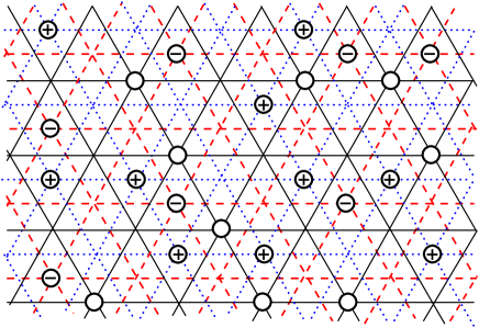
Figure 1: (Color online) Illustration of a two-dimensional ternary lattice gas with species labelled $\sigma\!=\!+,-,0$. Particles of each species occupy only one of the interlacing sublattices shown as dotted, broken, and solid lines, respectively; however, each particle may interact with all others via pairwize potentials $\phi_{\sigma\tau}(\mathbf{R}^{\sigma}-\mathbf{R}^{\tau})$.

In the case of binary fluids ($\mathcal{S}\!=\!2$), considered in Section III, major simplifications allow us to obtain explicitly all the thermodynamic and correlation properties in terms of the eigenvalues of the interaction matrix. The density correlations or (for charged fluids) charge correlations for the different species, appear as combinations of two eigenmodes. These contributions become uncoupled only in the often considered but usually unrealistic fully symmetric case.

To study critical behavior we go on in Section IV to consider systems with only hard cores and sufficiently attractive short-range interactions. With a proper choice of mixing coefficients, one can define $\check{m}$ and $\check{m}^{\dagger}$, two linear combinations of the species mean magnetizations or local densities, so that the usual spherical model critical singularities occur in the $(T,\check{m})$ plane at fixed $\check{m}^{\dagger}$. Thence, a critical locus emerges in the full $(T,\check{m},\check{m}^{\dagger})$ space which, together with a first-order surface, describes the influence of composition on the location of phase separation in the system. Via standard geometric arguments, criticality in the multicomponent model can then be deduced from corresponding one-component systems. Precisely, the same critical universality classes are realized as in short-range (attractive) spherical models.

Nevertheless, a significant difference arises in the equation of state where a new, unexpected mixing term appears. This can be understood heuristically as a type of demagnetization effect arising as a consequence of the vectorial character of the model coupled to asymmetry and multispecies features. This term indeed suppresses the normal divergence of susceptibilities at criticality; furthermore, it induces a linear dependence of the chemical potential and pressure as functions of the total density in the two-phase region! These are certainly undesirable and unphysical features of any fluid model. This wayward behavior reinforces the remark Fisher (1992) that, because of the de facto vectorial character of the order parameter in spherical models, their predictions must be handled with perspicacity when modeling fluids.

To gain some further insight into this unanticipated “demagnetization effect” we study in Section V an XY model beneath $T_{c}$ using a mean-field approach in which the vectorial character of the order parameter, coupled to an asymmetry of the external fields, leads transparently to a very similar demagnetization effect. Finally, some general conclusions are drawn in Section VI.

II Multicomponent spherical models

II.1 Fluid and spin systems

We consider a $d$-dimensional lattice fluid in the grand-canonical ensemble that consists of $\mathcal{S}$ species labeled $\sigma=1,\cdots,\mathcal{S}$, each being associated explicitly with only one of $\mathcal{S}$ identical interlaced sublattices (see Fig. 1). Every sublattice is taken as the image of a periodic reference sublattice ${\mathcal{R}^{0}}$ after translation by a vector ${\boldsymbol{\delta}}^{\sigma}$ so that every site $i$ on a lattice $\sigma$ is characterized by a position $\mathbf{R}^{\sigma}_{{i}}=\mathbf{R}_{i}^{0}+{\boldsymbol{\delta}}^{\sigma}$. The reference sublattice is generated by the vectors $\mathbf{a}_{\alpha}$ ($\alpha\!=\!1,\cdots,d$), has a unit cell volume $v_{0}$ and contains $\mathcal{N}\!=\!\prod_{\alpha}N_{\alpha}$ sites at positions $\mathbf{R}_{i}^{0}\!=\!\sum_{\alpha}\tilde{R}^{0}_{i,\alpha}\mathbf{a}_{\alpha}$ specified by the integers $\tilde{R}^{0}_{i,\alpha}\!=\!1,2,\cdots,N_{\alpha}$.

It is well-known that a grand-canonical lattice fluid is in correspondence with a canonical spin system See et al. (1952). Indeed, let us write the grand partition function of a fluid as

$$\Xi(T,\boldsymbol{\mu})=\prod_{\sigma}\left(\sum_{N_{\sigma}}\frac{1}{N_{\sigma}!}\sum_{\mathbf{r}_{i}^{\sigma}}\right)\exp\left[-\beta({\mathcal{H}}^{{\rm gas}}-\sum\nolimits_{\tau}\mu_{\tau}N_{\tau})\right],$$ (1)

where $\beta$ is the inverse temperature $1/k_{{\scriptscriptstyle B}}T$, while $N_{\sigma}$ and $\mu_{\sigma}$ denote the number of particles and chemical potential of species $\sigma$. The Hamiltonian ${\mathcal{H}}^{{\rm gas}}$ is expressed as a sum over particles $k\!=\!1,\cdots,n^{\sigma}$ and $l\!=\!1,\cdots,n^{\tau}$ as

$${\mathcal{H}}^{{\rm gas}}=\mbox{$\frac{1}{2}$}\sum_{(\sigma,k)\neq(\tau,l)}\varphi_{\sigma\tau}(\mathbf{r}^{\sigma}_{k}-\mathbf{r}^{\tau}_{l})\,,$$ (2)

where $\varphi_{\sigma\tau}$ is the pair interaction potential while $\mathbf{r}^{\sigma}_{k}$ is the position of the $k$-th particle of species $\sigma$, occupying sites on the lattice $\sigma$. Considering a system with hard cores, i.e., $\varphi_{\sigma\sigma}(\mathbf{0})\!=\!+\infty$, the sum in (1) refers to configurations where the local lattice density $n_{\sigma}(\mathbf{R}^{\sigma}_{{i}})=\sum_{k}\delta(\mathbf{R}^{\sigma}_{{i}}-\mathbf{r}^{\sigma}_{k})$ can be only $0$ or $1$, so that the local spin variable

$$s_{\sigma}(\mathbf{R}^{\sigma}_{{i}})=2n_{\sigma}(\mathbf{R}^{\sigma}_{{i}})-1\,,$$ (3)

takes the values $\pm 1$ as in the Ising model. A straightforward generalization of the procedure described in See et al. (1952) then leads to the partition function of a spin system, namely,

$$\Xi(T,\boldsymbol{\mu})=\prod_{\sigma}\sum_{s_{\sigma}(\mathbf{R}^{\sigma}_{{i}})=\pm 1}\exp\left(-\beta\,{\mathcal{H}}^{{\rm spin}}\right),$$ (4)

where the spin Hamiltonian is

$${\mathcal{H}}^{{\rm spin}}=-\mbox{$\frac{1}{2}$}\sum_{\begin{subarray}{c}(\sigma,i),(\tau,j)\end{subarray}}J_{\sigma\tau}(\mathbf{R}^{\sigma}_{{i}}-\mathbf{R}^{\tau}_{{j}})s_{\sigma}(\mathbf{R}^{\sigma}_{{i}})s_{\tau}(\mathbf{R}^{\tau}_{{j}})-\sum_{\sigma}h_{\sigma}\sum_{i}s_{\sigma}(\mathbf{R}^{\sigma}_{{i}})+\mathcal{H}_{o}(\boldsymbol{\mu})\,.$$ (5)

In this correspondence, the link between the coupling energies and pair interactions is

$$J_{\sigma\tau}(\mathbf{R}^{\sigma}_{{i}}-\mathbf{R}^{\tau}_{{j}})=-\mbox{$\frac{1}{4}$}\,\varphi_{\sigma\tau}(\mathbf{R}^{\sigma}_{{i}}-\mathbf{R}^{\tau}_{{j}})\quad\textrm{if \, $\mathbf{R}^{\sigma}_{{i}}\neq\mathbf{R}^{\tau}_{{j}}$ ,}$$ (6)

with $J_{\sigma\sigma}(\mathbf{0})\!=\!\mathbf{0}$, while the external fields are given by

$$h_{\sigma}=\mbox{$\frac{1}{2}$}\mu_{\sigma}-\mbox{$\frac{1}{4}$}\phi_{\sigma},$$ (7)

with reference level

$$\phi_{\sigma}=\sum_{(\tau,j)\neq(\sigma,i_{0})}\varphi_{\sigma\tau}(\mathbf{R}_{i_{0}}^{\sigma}-\mathbf{R}^{\tau}_{{j}})\,,$$ (8)

where $i_{0}$ is a fixed position. Finally, the background term in (5) is merely

$$\mathcal{H}_{o}(\boldsymbol{\mu})=-\mbox{$\frac{1}{2}$}\mathcal{N}\sum_{\sigma}\mu_{\sigma}+\mbox{$\frac{1}{8}$}\sum_{(\sigma,i)\neq(\tau,j)}\varphi_{\sigma\tau}(\mathbf{R}^{\sigma}_{{i}}-\mathbf{R}^{\tau}_{{j}})\,.$$ (9)

The correspondence between fluid and spin systems follows straightforwardly for the other properties. For instance, the local density $\rho_{\sigma}(\mathbf{r})\!=\!n_{\sigma}(\mathbf{r})/v_{0}$ is related to the local spin via

$$v_{0}\rho_{\sigma}(\mathbf{R}^{\sigma}_{{i}})=\mbox{$\frac{1}{2}$}\left[s_{\sigma}(\mathbf{R}^{\sigma}_{{i}})+1\right]\,,$$ (10)

while the species correlation functions

$$G_{\sigma\tau}(\mathbf{R}^{\sigma}_{{i}}-\mathbf{R}^{\tau}_{{j}};T,\boldsymbol{\mu})=\langle\rho_{\sigma}(\mathbf{R}^{\sigma}_{{i}})\rho_{\tau}(\mathbf{R}^{\tau}_{{j}})\rangle-\langle\rho_{\sigma}(\mathbf{R}^{\sigma}_{{i}})\rangle\langle\rho_{\tau}(\mathbf{R}^{\tau}_{{j}})\rangle\,,$$ (11)

are related to spin correlations via

$$v_{0}^{2}G_{\sigma\tau}(\mathbf{R}^{\sigma}_{{i}}-\mathbf{R}^{\tau}_{{j}};T,\boldsymbol{\mu})=\mbox{$\frac{1}{4}$}\left[\langle s_{\sigma}(\mathbf{R}^{\sigma}_{{i}})s_{\tau}(\mathbf{R}^{\tau}_{{j}})\rangle-\langle s_{\sigma}(\mathbf{R}^{\sigma}_{{i}})\rangle\langle s_{\tau}(\mathbf{R}^{\tau}_{{j}})\rangle\right]\,.$$ (12)

As usual, the angular brackets denote grand-canonical expectation values.

In order to define density or charge correlations simply in this lattice geometry, it is convenient to work in Fourier space. We consider periodic boundary conditions and define Fourier series with respect to the reference sublattice ${\mathcal{R}^{0}}$ by

$$\widehat{s}_{\sigma}(\mathbf{k})=\sum_{i}\textrm{e}^{-i\mathbf{k}\cdot\mathbf{R}^{\sigma}_{{i}}}s_{\sigma}(\mathbf{R}^{\sigma}_{{i}}).$$ (13)

Then, when $J_{\sigma\tau}$ is periodic over the reference sublattice, we may write

$$\widehat{J}_{\sigma\tau}(\mathbf{k})=\sum_{i}\textrm{e}^{-i\mathbf{k}\cdot(\mathbf{R}^{\sigma}_{{i}}-\mathbf{R}^{\tau}_{j_{0}})}J_{\sigma\tau}(\mathbf{R}^{\sigma}_{{i}}-\mathbf{R}^{\tau}_{j_{0}})=\sum_{j}\textrm{e}^{-i\mathbf{k}\cdot(\mathbf{R}^{\sigma}_{i_{0}}-\mathbf{R}^{\tau}_{{j}})}J_{\sigma\tau}(\mathbf{R}^{\sigma}_{i_{0}}-\mathbf{R}^{\tau}_{{j}})\,,$$ (14)

with any fixed positions $i_{0}$ and $j_{0}$. The wave vectors should be combinations of the reciprocal vectors $\mathbf{b}_{\alpha}$ (defined by $\mathbf{a}_{\alpha}\mathbf{\cdot}\mathbf{b}_{\alpha^{\prime}}\!=\!2\pi\delta_{\alpha,\alpha^{\prime}}$) such as $\mathbf{k}\!=\!\sum_{\alpha}\tilde{k}_{\alpha}\mathbf{b}_{\alpha}$ with $\tilde{k}_{\alpha}\!=\!0,\pm 1/N_{\alpha},\pm 2/N_{\alpha},\cdots$. In the following, the first Brillouin zone is denoted as $\mathcal{B}$. The density correlation function $G_{{\scriptscriptstyle NN}}$, and, for fluids of particles carrying charges $q_{\sigma}$, charge $G_{{\scriptscriptstyle ZZ}}$ and charge-density $G_{{\scriptscriptstyle NZ}}$ correlations can then be defined via

$$\widehat{G}_{{\scriptscriptstyle XY}}(\mathbf{k};T,\boldsymbol{\rho})=\sum_{\sigma,\tau}q_{\sigma}^{\vartheta_{{\scriptscriptstyle X}}}q_{\tau}^{\vartheta_{{\scriptscriptstyle Y}}}\widehat{G}_{\sigma\tau}(\mathbf{k};T,\boldsymbol{\rho})\,,$$ (15)

where $X$ and $Y$ stand either for $N$ or $Z$, with $\vartheta_{{\scriptscriptstyle N}}=0$, $\vartheta_{{\scriptscriptstyle Z}}=1$. We also define structure factors as

$$S_{{\scriptscriptstyle XY}}(\mathbf{k};T,\boldsymbol{\rho})=\frac{v_{0}}{\rho\,q^{\vartheta_{{\scriptscriptstyle X}}+\vartheta_{{\scriptscriptstyle Y}}}}\widehat{G}_{{\scriptscriptstyle XY}}(\mathbf{k};T,\boldsymbol{\rho})\,,$$ (16)

where $q$ is an elementary charge, while the total density is $\rho\!=\!\sum_{\sigma}\!\langle\rho_{\sigma}\rangle$. The term $v_{0}$ compensates here for the homogeneity difference between the discrete and continuum Fourier transforms.

II.2 Mean spherical model

We are not able to perform the multiple sums in (4) in general. Instead, we adopt the appropriate mean-spherical model Lewis and Wannier (1952) and compute the multiple integral

$$\Xi^{\prime}(T,\mathbf{h})=\int\prod_{\sigma}ds_{\sigma}\,\textrm{e}^{-\beta\,\mathcal{H}^{\prime}}\,,$$ (17)

with

$$\mathcal{H}^{\prime}={\mathcal{H}}^{{\rm spin}}+\sum_{\sigma}\tilde{\lambda}_{\sigma}\sum_{i}s_{\sigma}^{2}(\mathbf{R}^{\sigma}_{{i}})\,.$$ (18)

As usual, the Lagrange multipliers $\tilde{\lambda}_{\sigma}$ are introduced to allow imposition of the mean spherical conditions which need to be enforced uniformally for every species; specifically, the relations

$$\bigl{<}\sum_{i}s_{\sigma}^{2}(\mathbf{R}^{\sigma}_{{i}})\bigr{>}=\mathcal{N}\quad,\quad\sigma=1,\cdots\mathcal{S}\,.$$ (19)

define the Lagrange multipliers or spherical fields $\tilde{\lambda}_{\sigma}$ as implicit functions of $(T,\mathbf{h})$. Consequently, the free energy per site (of the reference sublattice) is

$$-\beta f\bigl{[}T,\mathbf{h},\boldsymbol{\lambda}(T,\mathbf{h})\bigr{]}=\ln\Xi^{\prime}(T,\mathbf{h})/\mathcal{N}\,,$$ (20)

in terms of which the spherical conditions (19) can be rewritten as

$$\langle s_{\sigma}^{2}\rangle=\left.\frac{\partial f}{\partial\tilde{\lambda}_{\sigma}}\right|_{T,\mathbf{h},{\tilde{\lambda}_{\tau}};\tau\neq\sigma}=1\quad,\quad\sigma=1,\ldots\mathcal{S}\,.$$ (21)

As already remarked in Sec. I, the spherical model in this form describes exactly spin models with fixed length or continuous $n$-component spins in the limit $n\rightarrow\infty$ with appropriate scalings Stanley (1968); See et al. (1978).

As standard Lewis and Wannier (1952), the calculation of $\Xi^{\prime}$ is performed in Fourier space. For consistency, we will suppose that $J_{\sigma\tau}$ satisfies the symmetry condition $J_{\sigma\tau}(\mathbf{R}^{\sigma}_{{i}}-\mathbf{R}^{\tau}_{{j}})\!=\!J_{\sigma\tau}\left[-(\mathbf{R}^{\sigma}_{{i}}-\mathbf{R}^{\tau}_{{j}})\right]$. The calculation is then a straightforward generalization of the mean-spherical techniques used for single-species systems. The free energy per site can be decomposed into a sum of three parts: $f\!=\!f_{s}+f_{h}+f_{o}$. The singular part of the free energy is

$$-\beta f_{s}(T,\mathbf{h})=-\frac{1}{2\mathcal{N}}\sum_{\mathbf{k}\in\mathcal{B}}\ln\left\{\beta^{\mathcal{S}}\textrm{Det}\left[\mathbf{\Lambda}(\mathbf{k};\boldsymbol{\lambda})\right]\right\}.$$ (22)

where the sum runs over the reference Brillouin zone $\mathcal{B}$ while $\mathbf{\Lambda}(\mathbf{k};\boldsymbol{\lambda})$ is the $\mathcal{S}\times\mathcal{S}$ interaction matrix with elements

$$\Lambda_{\sigma\tau}(\mathbf{k};\boldsymbol{\lambda})=\delta_{\sigma,\tau}\bigl{[}\lambda_{\sigma}+\Delta\widehat{J}_{\sigma\sigma}(\mathbf{k})\bigr{]}-\mbox{$\frac{1}{2}$}(1-\delta_{\sigma,\tau})\widehat{J}_{\sigma\tau}(\mathbf{k})\,,$$ (23)

in which for any function $\widehat{g}(\mathbf{k})$ we employ the notation

$$\Delta\widehat{g}(\mathbf{k})=\mbox{$\frac{1}{2}$}\left[\widehat{g}(\mathbf{0})-\widehat{g}(\mathbf{k})\right]\,,$$ (24)

while, dropping the tildes in (18) and (21), the shifted or net spherical fields are

$$\lambda_{\sigma}=\tilde{\lambda}_{\sigma}-\mbox{$\frac{1}{2}$}\widehat{J}_{\sigma\sigma}(\mathbf{0})\,.$$ (25)

On the other hand, the $h$-dependent part of the free energy is given by

$$-\beta f_{h}(T,\mathbf{h})=\mbox{$\frac{1}{4}$}\beta\langle\mathbf{h}|\mathbf{\Lambda}^{-1}(\mathbf{0},\boldsymbol{\lambda})|\mathbf{h}\rangle\,,$$ (26)

while the analytic background part, following from (9), is

$$-\beta f_{o}(T,\mathbf{h})=\mbox{$\frac{1}{2}$}\mathcal{S}\ln\pi-\beta\mathcal{H}_{o}/\mathcal{N}\,,$$ (27)

which will be neglected henceforth. Because of the logarithm in (22), these results are valid while the eigenvalues of the matrices $\mathbf{\Lambda}(\mathbf{k};\boldsymbol{\lambda})$ are positive for every $\mathbf{k}$; when one vanishes, the expressions (22) and (26) become singular and phase transitions are implicated.

The last step is taking the thermodynamic limit $\mathcal{N}\!\rightarrow\!\infty$ (valid provided the Fourier transforms remain well-defined) with the result

$$-\beta f_{s}(T,\mathbf{h})=-\mbox{$\frac{1}{2}$}\int_{\mathbf{k}}\ln\left\{\beta^{\mathcal{S}}\textrm{Det}\left[\mathbf{\Lambda}(\mathbf{k};\boldsymbol{\lambda})\right]\right\}\,,$$ (28)

where $\int_{\mathbf{k}}$ is a short-hand notation for $\int_{\mathbf{k}\in\mathcal{B}}v_{0}d^{d}\mathbf{k}/(2\pi)^{d}$, while the $\mathbf{h}$-dependent free energy $f_{h}$ is still given by (26). At this point, it is worth noting that the structure of $f_{s}$, as an integral over the Brillouin zone of the logarithm of the interactions in Fourier space, is similar to that present in Onsager’s exact solution of the 2D Ising model Onsager (1944). The consequences for charged systems are dramatic Aqua and Fisher (2004a, b, ) since this form determines the coupling or decoupling of correlations in symmetric and asymmetric systems.

With these results in hand, we find that the mean particle densities $\rho_{\sigma}=\langle\rho_{\sigma}(\mathbf{R}^{\sigma}_{{i}})\rangle$ are related to the mean magnetizations via

$$2\rho_{\sigma}v_{0}-1=m_{\sigma}=\langle s_{\sigma}\rangle=-\left.\frac{\partial f_{h}}{\partial h_{\sigma}}\right|_{T,h_{\tau},\boldsymbol{\lambda};\tau\neq\sigma}\,,$$ (29)

which, in turn, enter the free energy in standard manner as

$$f_{h}=-\mbox{$\frac{1}{2}$}\sum_{\sigma}m_{\sigma}h_{\sigma}\,.$$ (30)

As a result of (26) and (29), the link between $\mathbf{h}$ and $\mathbf{m}$ is then merely

$$\mathbf{h}=\mbox{$\frac{1}{2}$}\boldsymbol{\mu}-\mbox{$\frac{1}{4}$}\boldsymbol{\phi}=2\mathbf{\Lambda}(\mathbf{0})\mathbf{m},$$ (31)

where $\boldsymbol{\mu}\!=\!\{\mu_{\sigma}\}$ and we have recalled (7) and introduced a fixed vector $\boldsymbol{\phi}\!=\!\{\phi_{\sigma}\}$: see (8). Finally, in the thermodynamic limit, the spin-spin correlation functions are given by

$$\langle s_{\sigma}(\mathbf{R}^{\sigma}_{{i}})s_{\tau}(\mathbf{R}^{\tau}_{{j}})\rangle=-\frac{1}{2-\delta_{\sigma,\tau}}\left.\frac{\partial(f-f_{o})}{\partial J_{\sigma\tau}(\mathbf{R}^{\sigma}_{{i}}-\mathbf{R}^{\tau}_{{j}})}\right|_{T,\mathbf{h},\boldsymbol{\lambda}}\,,$$ (32)

where $2-\delta_{\sigma,\tau}$ is merely a symmetry factor, while we recall (12) for the density correlation functions $G_{\sigma\tau}$.

III Binary systems

The previous analysis holds for an arbitrary number of species. From here on, however, we focus on the simplest case, i.e., binary mixtures with species labels $1$ and $2$. For many properties, it is useful to decompose densities, chemical potentials, etc., in terms of means and differences; so for every function $g_{\sigma}$ (or $g_{\sigma\sigma}$) we define

$$\bar{g}=\mbox{$\frac{1}{2}$}\left(g_{1}+g_{2}\right),\quad\quad g^{\dagger}=\mbox{$\frac{1}{2}$}\left(g_{1}-g_{2}\right)\,.$$ (33)

Moreover, for simplicity, we suppose that the translation vectors ${\boldsymbol{\delta}}^{\sigma}\!=\!\sum_{\alpha}\tilde{\delta}_{\alpha}\mathbf{a}_{\alpha}$ satisfy $\tilde{\delta}_{\alpha}\!=\!0$ or $1/2$ so that the Fourier transforms $\widehat{J}_{\sigma\tau}$ are real.

III.1 Basic features

For the case $\mathcal{S}\!=\!2$, simplifications allow more explicit results. First, let us introduce the energy scale

$$j_{0}=\mbox{$\frac{1}{2}$}\widehat{J}_{{\scriptstyle{12}}}(\mathbf{0})\,,$$ (34)

and, following (33), write

$$\Delta\bar{J}(\mathbf{k})=\mbox{$\frac{1}{2}$}\left(\Delta J_{{\scriptstyle{11}}}+\Delta J_{{\scriptstyle{22}}}\right),$$ (35a)

$$\Delta J^{\dagger}(\mathbf{k})=\mbox{$\frac{1}{2}$}\left(\Delta J_{{\scriptstyle{11}}}-\Delta J_{{\scriptstyle{22}}}\right).$$ (35b)

Then the eigenvalues of the $2\times 2$ matrix $\boldsymbol{\Lambda}$ may be written

$$\Lambda_{\pm}(\mathbf{k};\boldsymbol{\lambda})=\bar{\lambda}+\Delta\bar{J}(\mathbf{k})\pm D(\mathbf{k};\boldsymbol{\lambda})\,,$$ (36)

where

$$D(\mathbf{k};\boldsymbol{\lambda})=\sqrt{\left[\lambda^{\dagger}+\Delta J^{\dagger}(\mathbf{k})\right]^{2}+\mbox{$\frac{1}{4}$}[\widehat{J}_{{\scriptstyle{12}}}(\mathbf{k})]^{2}}\geq 0.$$ (37)

As remarked above, these expressions are valid when $\Lambda_{-}$ and $\Lambda_{+}$ are nonnegative while singularities arise only when $\Lambda_{-}(\mathbf{k};\boldsymbol{\lambda})\,[\leq\Lambda_{+}(\mathbf{k};\boldsymbol{\lambda})]\rightarrow 0$.

Now the argument of the free energy integral in (28) is $\ln\{\beta^{2}\textrm{Det}[\mathbf{\Lambda}]\}$, where the determinant of the interaction matrix can now be written

$$\Lambda_{-}\Lambda_{+}(\mathbf{k};\boldsymbol{\lambda})=u+2\bar{\lambda}\Delta\bar{J}(\mathbf{k})-2\lambda^{\dagger}\Delta J^{\dagger}(\mathbf{k})+\Delta J^{\,2}(\mathbf{k}),$$ (38)

where we have introduced the crucial parameter

$$u(\boldsymbol{\lambda})\equiv\Lambda_{-}\Lambda_{+}(\mathbf{0};\boldsymbol{\lambda})=\bar{\lambda}^{2}-\lambda^{\dagger^{{\scriptstyle{2}}}}-{j_{0}}^{2}\,,$$ (39)

which vanishes when $\textrm{Det}[\mathbf{\Lambda}(\mathbf{k})]$ vanishes at $\mathbf{k}\!=\!\mathbf{0}$, while the squared interaction term in (38), namely,

$$\Delta J^{\,2}(\mathbf{k})={j_{0}}^{2}-\mbox{$\frac{1}{4}$}{\widehat{J}_{{\scriptstyle{12}}}}^{\,2}(\mathbf{k})+\Delta\widehat{J}_{{\scriptstyle{11}}}(\mathbf{k})\Delta\widehat{J}_{{\scriptstyle{22}}}(\mathbf{k}),$$ (40)

vanishes as $|\mathbf{k}^{2}|$.

In terms of the eigenvalues, the spherical conditions (21) become

$$1=\mbox{$\frac{1}{2}$}k_{{\scriptscriptstyle B}}T\int_{\mathbf{k}}\frac{\lambda_{\sigma}+\Delta\widehat{J}_{\sigma\sigma}(\mathbf{k})}{\Lambda_{-}\Lambda_{+}(\mathbf{k};\boldsymbol{\lambda})}+m_{\tau}^{2}\,,\quad\tau\neq\sigma.$$ (41)

Finally, the $h$-dependent part of the free energy entails

$$\mathbf{\Lambda}^{-1}(\mathbf{0};\boldsymbol{\lambda})=\frac{1}{\Lambda_{-}\Lambda_{+}(\mathbf{0};\boldsymbol{\lambda})}\begin{pmatrix}\lambda_{2}\,\,&j_{0}\\ j_{0}\,\,&\lambda_{1}\end{pmatrix}\,,$$ (42)

while the magnetization-field or density-chemical potential relation (31) becomes

$$\mbox{$\frac{1}{2}$}h_{\sigma}=m_{\sigma}\lambda_{\sigma}-m_{\tau}j_{0}\,,\quad\tau\neq\sigma.$$ (43)

At this point, Eqs. (34)-(43) entirely define the system and the need is to analyze their structure and consequences.

III.2 Correlation functions

The density pair correlation functions are given generally by (12) and (32) which, when $\mathcal{S}\!=\!2$, reduce to

$$\widehat{G}_{\sigma\sigma}(\mathbf{k};\boldsymbol{\lambda})=\frac{k_{{\scriptscriptstyle B}}T}{8v_{0}^{2}}\frac{\lambda_{\sigma}+\Delta\widehat{J}_{\sigma\sigma}(\mathbf{k})}{\Lambda_{-}\Lambda_{+}(\mathbf{k};\boldsymbol{\lambda})},\quad(\sigma=1,2),$$ (44)

$$\widehat{G}_{{\scriptstyle{12}}}(\mathbf{k};\boldsymbol{\lambda})=\frac{k_{{\scriptscriptstyle B}}T}{16v_{0}^{2}}\frac{\widehat{J}_{{\scriptstyle{12}}}(\mathbf{k})}{\Lambda_{-}\Lambda_{+}(\mathbf{k};\boldsymbol{\lambda})}=\widehat{G}_{{\scriptstyle{21}}}(\mathbf{k};\boldsymbol{\lambda}).$$ (45)

In terms of these, one can use (15) to obtain the overall density-density correlation function, $\widehat{G}_{{\scriptscriptstyle NN}}$ and, the complementary compositional correlations or, for charged systems, the charge-charge correlation function $\widehat{G}_{{\scriptscriptstyle ZZ}}$.

From a purely mathematical perspective, it is also instructive to decompose the fluctuations with respect to the eigenvectors of $\mathbf{\Lambda}$ which, of course, depend on the wavevector $\mathbf{k}$ and the fields $\boldsymbol{\lambda}$. Thus if we define $\phi(\mathbf{k})$ via

$$\tan\phi(\mathbf{k})=2\left\{D(\mathbf{k};\boldsymbol{\lambda})-\bigl{[}\lambda^{\dagger}+\Delta J^{\dagger}(\mathbf{k})\bigr{]}\right\}/\widehat{J}_{{\scriptstyle{12}}}(\mathbf{k}),$$ (46)

it can be interpreted as the angle determined by the eigenvector associated with $\Lambda_{+}(\mathbf{k};\boldsymbol{\lambda})$ relative to the $\sigma\!=\!1$ axis. Then if we introduce the density fluctuations $\rho^{+}(\mathbf{k};\boldsymbol{\lambda})$ and $\rho^{-}(\mathbf{k};\boldsymbol{\lambda})$ via

$$\rho^{\pm}=\left[\rho_{1}\cos\phi(\mathbf{k};\boldsymbol{\lambda})\mp\rho_{2}\sin\phi(\mathbf{k};\boldsymbol{\lambda})\right]/\sqrt{2},$$ (47)

and define the corresponding correlation function $\widehat{G}_{\pm\pm}$ in the natural way, we find

$$\widehat{G}_{++}(\mathbf{k};\boldsymbol{\lambda})=\frac{k_{{\scriptscriptstyle B}}T}{16v_{0}^{2}}\frac{1}{\Lambda_{+}(\mathbf{k};\boldsymbol{\lambda})}\,,$$ (48a)

$$\widehat{G}_{--}(\mathbf{k};\boldsymbol{\lambda})=\frac{k_{{\scriptscriptstyle B}}T}{16v_{0}^{2}}\frac{1}{\Lambda_{-}(\mathbf{k};\boldsymbol{\lambda})}\,.$$ (48b)

while $\widehat{G}_{+-}\!=\!\widehat{G}_{-+}$ vanishes identically.

However, the eigenmodes (47) will rarely be of direct physical significance. Rather the physically accessible fluctuations, represented in particular by the structure functions introduced in (15) and (16), will typically involve a mixture of the underlying eigenmodes. Specifically we find

$$\frac{S_{{\scriptscriptstyle NN}}(\mathbf{k};T,\boldsymbol{\rho})}{k_{{\scriptscriptstyle B}}T/4\rho v_{0}}=\frac{B(\mathbf{k};\boldsymbol{\lambda})}{\Lambda_{-}(\mathbf{k};\boldsymbol{\lambda})}+\frac{1-B(\mathbf{k};\boldsymbol{\lambda})}{\Lambda_{+}(\mathbf{k};\boldsymbol{\lambda})}\,,\\$$ (49a)

and, for charged systems with $$q_{+}\!=\!-q_{-}\!=\!q$$,

$$\frac{S_{{\scriptscriptstyle ZZ}}(\mathbf{k};T,\boldsymbol{\rho})}{k_{{\scriptscriptstyle B}}T/4\rho v_{0}}=\frac{B(\mathbf{k};\boldsymbol{\lambda})}{\Lambda_{+}(\mathbf{k};\boldsymbol{\lambda})}+\frac{1-B(\mathbf{k};\boldsymbol{\lambda})}{\Lambda_{-}(\mathbf{k};\boldsymbol{\lambda})}\,,$$ (49b)

where the mixing amplitude $B$ is

$$B(\mathbf{k};\boldsymbol{\lambda})=\mbox{$\frac{1}{2}$}+\mbox{$\frac{1}{4}$}\widehat{J}_{{\scriptstyle{12}}}(\mathbf{k})/D(\mathbf{k};\boldsymbol{\lambda})\,.$$ (50)

Evidently, singular behavior, anticipated at criticality in $\Lambda_{-}(\mathbf{k};\boldsymbol{\lambda})$, will in general affect both $S_{{\scriptscriptstyle NN}}$ and $S_{{\scriptscriptstyle ZZ}}$ as we discuss in detail elsewhere Aqua and Fisher (2004a, b, ).

However, a special situation arises when the two species 1 and 2 are symmetrically related so that $\widehat{J}_{{\scriptstyle{11}}}(\mathbf{k})\!=\!\widehat{J}_{{\scriptstyle{22}}}(\mathbf{k})$ which implies, via (35b), $\Delta J^{\dagger}(\mathbf{k})\equiv 0$. For a charged system this corresponds to complete charge symmetry as exemplified most simply in the restricted primitive model (RPM) of equisized hard spheres with charges of equal magnitude but opposite sign. But neutral systems where species 1 and 2 differ only in chirality demand a symmetric description quite naturally. Then, on the locus of symmetry where $\rho_{1}\!=\!\rho_{2}$ (corresponding to electroneutrality in 1:1 ionic fluids) one has $\mu_{1}\!=\!\mu_{2}$ and, hence, via (31), $\lambda_{1}\!=\!\lambda_{2}$ and thence, via (33) $\lambda^{\dagger}\equiv 0$. In this case one sees from (50) that $B(\mathbf{k};\boldsymbol{\lambda})$ vanishes identically so that the eigenmodes precisely specify $S_{{\scriptscriptstyle NN}}$ and $S_{{\scriptscriptstyle ZZ}}$ which, therefore, become totally decoupled! This turns out to play a crucial role in the study of charge screening near ionic criticality Aqua and Fisher (2004a, b, ) albeit for generally unrealistic charge-symmetric systems.

A small technical detail deserves mentioning in this fully symmetric case if $\widehat{J}_{{\scriptstyle{12}}}(\mathbf{k})$ should change sign for $\mathbf{k}\!\neq\!\mathbf{0}$ (which is not unreasonable); then the ratio $\widehat{J}_{{\scriptstyle{12}}}/D(\mathbf{k};\boldsymbol{\lambda})$ in (50) together with $\Lambda_{+}$ and $\Lambda_{-}$ involve nonanalytic absolute values but in such a way that the combinations $S_{{\scriptscriptstyle NN}}$ and $S_{{\scriptscriptstyle ZZ}}$ in (49) remain completely analytic.

Finally, the cross charge-density structure function is also expressible as a combination of the two eigenmodes via

$$\frac{S_{{\scriptscriptstyle NZ}}(\mathbf{k};T,\boldsymbol{\rho})}{k_{{\scriptscriptstyle B}}T/8v_{0}\rho}=\frac{\lambda^{\dagger}+\Delta J^{\dagger}(\mathbf{k})}{D(\mathbf{k};\boldsymbol{\lambda})}\left[\frac{1}{\Lambda_{-}(\mathbf{k};\boldsymbol{\lambda})}-\frac{1}{\Lambda_{+}(\mathbf{k};\boldsymbol{\lambda})}\right]\,.$$ (51)

As is to be anticipated, this vanishes identically on the symmetry locus when (1, 2) symmetry is present.

III.3 Appropriately mixed thermodynamic variables

Depending on the symmetry of the system, the previous relations may be handled more or less conveniently. In the general asymmetric case ($\widehat{J}_{{\scriptstyle{11}}}\neq\widehat{J}_{{\scriptstyle{22}}}$), the spherical constraints (41) can be rewritten as

$$1=\mbox{$\frac{1}{2}$}k_{{\scriptscriptstyle B}}T\int_{\mathbf{k}}\frac{\bar{\lambda}+\Delta\bar{J}(\mathbf{k})}{\Lambda_{-}\Lambda_{+}(\mathbf{k};\boldsymbol{\lambda})}+m^{2}+{m^{\dagger}}^{2}\,,$$ (52)

and

$$2mm^{\dagger}=\mbox{$\frac{1}{2}$}k_{{\scriptscriptstyle B}}T\int_{\mathbf{k}}\frac{\lambda^{\dagger}+\Delta J^{\dagger}(\mathbf{k})}{\Lambda_{-}\Lambda_{+}(\mathbf{k};\boldsymbol{\lambda})}\,,$$ (53)

while the external fields are given by

$$\bar{h}= 2\left[m(\bar{\lambda}-j_{0})+m^{\dagger}\lambda^{\dagger}\right]\,,$$ (54a)

$$h^{\dagger}= 2\left[m\lambda^{\dagger}+m^{\dagger}(\bar{\lambda}+j_{0})\right]\,.$$ (54b)

Note that, since $\Lambda_{-}$ and $\Lambda_{+}$ are nonnegative, the condition (52) is consistent with the expectations $|m|\!\leq\!1$ and $|m^{\dagger}|\!\leq\!1$.

For further analysis it is convenient to introduce the basic integral functions

$$\mathcal{G}(\boldsymbol{\lambda})=\mbox{$\frac{1}{2}$}\int_{\mathbf{k}}\frac{1}{\Lambda_{-}\Lambda_{+}(\mathbf{k};\boldsymbol{\lambda})}\,,$$ (55)

$$\mathcal{L}_{\sigma}(\boldsymbol{\lambda})=\mbox{$\frac{1}{2}$}\int_{\mathbf{k}}\frac{\Delta\widehat{J}_{\sigma\sigma}(\mathbf{k})}{\Lambda_{-}\Lambda_{+}(\mathbf{k};\boldsymbol{\lambda})}\,,$$ (56)

which are simple generalizations of the typical integrals involved in the analysis of standard spherical models.

Now, in the fully symmetric case, $\Delta J^{\dagger}$, $\lambda^{\dagger}$, and $m^{\dagger}$ vanish identically so that the relations (53) and (54b) have no role to play. Then (52) and (54a) closely resemble the basic expressions for the single-species ($\mathcal{S}\!=\!1$) or standard spherical model. These in turn lead to the basic equation of state which, in terms of the reduced temperature variable

$$t=(T-T_{c})/T_{c},$$ (57)

can be written most transparently near the critical point ($T\!=\!T_{c}$, $m\!=\!0$) as Fisher (2005); Fisher and Aqua ; Joyce (1972)

$$p_{0}u^{1/\gamma}\approx c_{t}t+c_{m}m^{2},$$ (58)

where, recalling (39), $u\!=\!\bar{\lambda}^{2}-j_{0}^{2}$ while $\gamma\!\geq\!1$ is the fundamental dimensionality-dependent exponent, and $p_{0}$, $c_{t}$, and $c_{m}$ are fixed positive coefficients.

Now physicochemical insight into the behavior of binary fluid mixtures suggests strongly that their critical behavior will, when expressed in terms of suitable density and field variables be essentially the same as for a single-component fluid. However, the “suitable” or “appropriate” variables will, in leading order, be linear combinations or mixtures of the related binary thermodynamic variables, specifically, the fields and densities. Furthermore, the appropriate mixing coefficients must, in general, be nontrivial functions of the state variables.

It follows that our primary task now is to find what the appropriate mixing coefficients are. To that end, we introduce the general linear combinations

$$\check{\lambda}=\mbox{$\frac{1}{2}$}\left(\theta^{-1}\lambda_{1}+\theta\lambda_{2}\right),\quad{\check{\lambda}^{\dagger}}=\mbox{$\frac{1}{2}$}\left(\theta^{-1}\lambda_{1}-\theta\lambda_{2}\right),$$ (59)

together with corresponding remixed interactions

$$\Delta\check{J},\,\Delta\check{J}^{\dagger}=\mbox{$\frac{1}{2}$}\left(\theta^{-1}\Delta J_{{\scriptstyle{11}}}\pm\theta\Delta J_{{\scriptstyle{22}}}\right).$$ (60)

The mixing parameter $\theta$ is to be determined later. In terms of these new variables and interactions, the basic determinant becomes

$$\textrm{Det}[\mathbf{\Lambda}]=u+2\check{\lambda}\Delta\check{J}(\mathbf{k})-2{\check{\lambda}^{\dagger}}\Delta\check{J}^{\dagger}(\mathbf{k})+\Delta J^{\,2}(\mathbf{k}),$$ (61)

where, following (39), the value at $\mathbf{k}\!=\!\mathbf{0}$ is now

$$u(\lambda_{1},\lambda_{2})=\check{\lambda}^{2}-\check{\lambda}^{\dagger^{{\scriptstyle{2}}}}-{j_{0}}^{2}.$$ (62)

Then it proves necessary to introduce a second state-dependent mixing parameter $\theta_{m}$ by writing

$$\check{m},\check{m}^{\dagger}=\mbox{$\frac{1}{2}$}\left(\theta_{m}^{-1}m_{1}\pm\theta_{m}m_{2}\right).$$ (63)

In terms of these new variables and the integrals (55) and (56), the original spherical conditions (41) become

$$1=\theta^{-1}k_{{\scriptscriptstyle B}}T(\check{\lambda}-{\check{\lambda}^{\dagger}})\mathcal{G}(\boldsymbol{\lambda})+\mathcal{L}_{2}(\boldsymbol{\lambda})k_{{\scriptscriptstyle B}}T$$

$$+\theta_{m}^{2}(\check{m}^{2}+\check{m}^{\dagger^{{\scriptstyle{2}}}}+2\check{m}\check{m}^{\dagger}),$$ (64a)

$$1=\theta k_{{\scriptscriptstyle B}}T(\check{\lambda}+{\check{\lambda}^{\dagger}})\mathcal{G}(\boldsymbol{\lambda})+\mathcal{L}_{1}(\boldsymbol{\lambda})k_{{\scriptscriptstyle B}}T$$

$$+\theta_{m}^{-2}(\check{m}^{2}+\check{m}^{\dagger^{{\scriptstyle{2}}}}-2\check{m}\check{m}^{\dagger}).$$ (64b)

Finally, it is helpful to define new external fields via

$$\check{h}=\mbox{$\frac{1}{2}$}\left(\theta_{h}^{-1}h_{1}+\theta_{h}h_{2}\right),\quad\check{h}^{\dagger}=\mbox{$\frac{1}{2}$}\left(\theta_{h}^{-1}h_{1}-\theta_{h}h_{2}\right),$$ (65)

which are linked to the generalized magnetizations via

$$\check{h}=\check{m}\left[(\check{\lambda}-j_{0})\,\omega_{+}+{\check{\lambda}^{\dagger}}\omega_{-}+j_{0}\pi^{+}_{m}\right]\\ +\check{m}^{\dagger}\left[(\check{\lambda}-j_{0})\,\omega_{-}+{\check{\lambda}^{\dagger}}\omega_{+}+j_{0}\pi^{+}_{m^{\dagger}}\right]\,,\mbox{\hskip 56.9055pt}$$ (66)

and similarly for $\check{h}^{\dagger}$ in terms of $\pi_{m}^{-}$ and $\pi_{m^{\dagger}}^{-}$ with $\omega_{+}$ and $\omega_{-}$ interchanged while the coefficients $\omega_{\pm}$, $\pi_{m}^{\pm}$, and $\pi_{m^{\dagger}}^{\pm}$ are found to be

$$\omega_{\pm}=\theta\theta_{m}/\theta_{h}\pm\,\theta_{h}/\theta\theta_{m}\,,$$ (67)

$$\pi^{\pm}_{m}/(\theta_{m}-1/\theta\theta_{m})=\pi^{\pm}_{m^{\dagger}}/(\theta_{m}+1/\theta\theta_{m})$$

$$=\theta/\theta_{h}\mp\,\theta_{h}\,.$$ (68)

With these new fields and magnetizations, the free energy per site reduces to

$$f_{h}=-\mbox{$\frac{1}{2}$}\left(\theta_{h}\theta_{m}+1/\theta_{h}\theta_{m}\right)(\check{m}\check{h}+\check{m}^{\dagger}\check{h}^{\dagger})\\ +\mbox{$\frac{1}{2}$}\left(\theta_{h}\theta_{m}-1/\theta_{h}\theta_{m}\right)(\check{m}\check{h}^{\dagger}+\check{m}^{\dagger}\check{h}).\hskip 85.35826pt$$ (69)

As we will show, the choice of the coefficients $\theta$, $\theta_{m}$ and $\theta_{h}$ will be dictated by physical arguments in order to ensure compact and familiar expressions for the critical behavior.

IV Binary lattice gases with short-range attractive interactions

To obtain explicit results for critical behavior we focus now on binary systems with short-range interactions (in addition to the hard cores already accounted for). Accordingly, we suppose that the small-$\mathbf{k}$ expansions of the interactions in $\mathbf{k}$ space are

$$\widehat{J}_{\sigma\tau}(\mathbf{k})=\widehat{J}_{\sigma\tau}(\mathbf{0})\left[1-k^{2}\,R_{\sigma\tau}^{2}+{\mathcal{O}}(k^{4})\right],\quad(\sigma,\tau=1,2),$$ (70)

with fixed range parameters $R_{\sigma\tau}$. Moreover, to ensure simple criticality, we suppose that the interactions are “overall attractive”, which we take to mean that $j_{0}$, $\Delta\widehat{J}_{{\scriptstyle{12}}}$ and $\Delta\bar{J}$ are real and satisfy

$$j_{0}=\mbox{$\frac{1}{2}$}\widehat{J}_{{\scriptstyle{12}}}(\mathbf{0})\!>\!0\,\,\,\textrm{and }\,\Delta|\widehat{J}_{{\scriptstyle{12}}}(\mathbf{k})|>0,\,\,\,\Delta\bar{J}(\mathbf{k})>0\quad\forall\mathbf{k}\neq\mathbf{0}.$$ (71)

These conditions are easily fulfilled, as, for example, when $J_{{\scriptstyle{12}}}(\mathbf{r})\!=\!J_{{\scriptstyle{12}}}(-\mathbf{r})$ while $J_{{\scriptstyle{11}}}(\mathbf{r})$ and $J_{{\scriptstyle{22}}}(\mathbf{r})$ are positive for all $\mathbf{r}$.

IV.1 Critical loci

To identify the singularities of the binary systems, we recall that they are signaled by the vanishing of one of the eigenvalues of $\mathbf{\Lambda}$, which occurs first when $\Lambda_{-}(\mathbf{k};\boldsymbol{\lambda})$ vanishes. As shown in Appendix A, these singularities arise only when $(i)$ $\mathbf{k}\!=\!\mathbf{0}$, and, thence, $(ii)$ when the spherical fields $\boldsymbol{\lambda}$ satisfy

$$u(\lambda_{1},\lambda_{2})=0\,,$$ (72)

provided the asymmetries of the interactions are not too extreme in the sense that, as we suppose henceforth, $\Delta J^{\dagger}(\mathbf{k})$ [defined in (35b)] satisfies the conditions (113) and (118).

Now, any state of the system is specified ab initio by the three thermodynamic fields $(T,\mu_{1},\mu_{2})$ which, via (21), give $\boldsymbol{\lambda}(T,\mathbf{h})$, and then the densities $\mathbf{m}$. However, for the location of critical points, it is more convenient to utilize the set of variables $(T,\check{m},\check{m}^{\dagger})$ introduced in (63) and then to solve for $(\check{\lambda},{\check{\lambda}^{\dagger}})$ as defined in (59).

Next, let us choose $\theta_{m}\!>\!0$ in (63) so that $\check{m}_{c}$ vanishes at criticality or, in other words, take $\theta_{m}\!=\!(-m_{1,c}/m_{2,c})^{1/2}$. This condition will be analyzed below in seeking a critical point, at a given value of $\check{m}^{\dagger}$. Likewise, we choose $\theta\!>\!0$ in (59) so that ${\check{\lambda}^{\dagger}}_{c}=0$. This condition then enforces the link between $\theta$ and $\check{m}^{\dagger}$, since it implies $\theta^{2}\!=\!\lambda_{1,c}/\lambda_{2,c}$. As established in Appendix A, the singularities are characterized by $u\!=\!0$, which via (62) means $\check{\lambda}_{c}=j_{0}$ and thence, $\lambda_{1,c}=\theta j_{0}$ and $\lambda_{2,c}=j_{0}/\theta$.

At this point, one must pay attention to the behavior of integral expressions (55) and (56) when $\Lambda_{-}(\mathbf{0})$ approaches zero. If we accept (70) we find that $\Lambda_{-}$ varies as $k^{2}$ when $\Lambda_{-}(\mathbf{0})\!=\!0$ and then $\mathcal{G}(\boldsymbol{\lambda})$ and $\mathcal{L}_{\sigma}(\boldsymbol{\lambda})$ remain finite at the singularity provided $d\!>\!d_{<}\!=\!2$ (in this case) as seen in Barbosa and Fisher (1991). Accordingly, from here on we suppose the dimensionality exceeds $d\!=\!2$ and may then write

$$\mathcal{G}(\boldsymbol{\lambda}_{c})=g_{0}(\theta)/j_{0}^{2},\quad\mathcal{L}_{\sigma}(\boldsymbol{\lambda}_{c})=g_{0}(\theta)l_{\sigma,0}(\theta)/j_{0},\quad(\sigma=1,2).$$ (73)

The residual $\theta$-dependence arises from $\Delta\check{J}$ and $\Delta\check{J}^{\dagger}$, see (60), (61), (55) and (56).

Putting these considerations together we find that the critical locus, $T_{c}(\check{m}^{\dagger})$ with $\check{m}_{c}\!=\!0$, may be defined parametrically via

$$k_{{\scriptscriptstyle B}}T_{c}(\check{m}^{\dagger})=\frac{j_{0}(1-\theta_{m}^{2}\check{m}^{\dagger^{{\scriptstyle{2}}}})}{g_{0}(\theta)[1/\theta+l_{2,0}(\theta)]}\,,$$ (74)

$$\check{m}^{\dagger^{{\scriptstyle{2}}}}=\frac{(\theta-1/\theta)+l_{1,0}(\theta)-l_{2,0}(\theta)}{(\theta\theta_{m}^{2}-1/\theta\theta_{m}^{2})+l_{1,0}(\theta)\theta_{m}^{2}-l_{2,0}(\theta)/\theta_{m}^{2}}\,.$$ (75)

In fact, the latter relation must be seen as an implicit equation giving $\theta$ as a function of $\check{m}^{\dagger}$ while, as shown below, $\theta_{m}$ will also be related to $\theta$. Hence, if one realizes that $\check{m}^{\dagger}$ (i.e., some combination of the densities other than the total density) characterizes the composition of the system, the function $T_{c}(\check{m}^{\dagger})$ describes naturally the composition dependence of criticality in the binary fluids.

IV.2 Critical neighborhood

We seek an expression for the physical properties of the binary system in terms of $(T,\check{m},\check{m}^{\dagger})$ near the critical locus $(T_{c},0,\check{m}^{\dagger})$. For this purpose, we first solve for ${\check{\lambda}^{\dagger}}$ in terms of $T$, $\check{m}$ and $\check{m}^{\dagger}$: this can be done implicitly in the general case by invoking (64), and explicitly in the vicinity of a critical point by implementing a perturbation scheme at fixed $\check{m}^{\dagger}$. To this end, consider the critical point at $T_{c}(\check{m}^{\dagger})$ and $\check{m}_{c}\!=\!0$ and its vicinity defined by the two small parameters, $t\!\varpropto(T-T_{c})$, as introduced in (57) and $\check{m}$. By construction, $u$ and ${\check{\lambda}^{\dagger}}$ are small parameters near criticality, so that the integral involved in $\mathcal{G}(\boldsymbol{\lambda})$ can be computed as usual in spherical models, see Fisher (2005); Joyce (1972); Barbosa and Fisher (1991). However, a significant new feature is that the integral is now a function of two vanishing parameters, $u$ and ${\check{\lambda}^{\dagger}}$. The appropriate extension of the standard critical expansion Barbosa and Fisher (1991) yields

$$\mathcal{G}(\boldsymbol{\lambda})=g_{0}j_{0}^{-2}\left[1-p(1-p^{\dagger}{\check{\lambda}^{\dagger}})u^{1/\gamma}+q_{0}u+g_{1}{\check{\lambda}^{\dagger}}/j_{0}+g_{2}\check{\lambda}^{\dagger^{{\scriptstyle{2}}}}/j_{0}^{2}\right.\\ +\left.{\mathcal{O}}\left(u^{1/\gamma}\check{\lambda}^{\dagger^{{\scriptstyle{2}}}},\check{\lambda}^{\dagger^{{\scriptstyle{3}}}}\right)+o(u)\right]\,,$$ (76)

with coefficients $p$, $p^{\dagger}$, $q_{0}$, $g_{1}$, and $g_{2}$ which in general still depend on $\theta$, and with the critical exponent

$$\gamma=\max\left[2/(d-2);1\right]\,.$$ (77)

The integrals $\mathcal{L}_{\sigma}(\boldsymbol{\lambda})$ are less singular and one finds

$$\mathcal{L}_{\sigma}(\boldsymbol{\lambda})=g_{0}j_{0}^{-1}\left[l_{\sigma,0}+l_{\sigma,1}{\check{\lambda}^{\dagger}}/j_{0}+l_{\sigma,2}\check{\lambda}^{\dagger^{{\scriptstyle{2}}}}/j_{0}^{2}+{\mathcal{O}}(u,\check{\lambda}^{\dagger^{{\scriptstyle{3}}}})\right]\,.$$ (78)

We note that $g_{1}$ and $l_{\sigma,1}$ vanish in the symmetric case when $\Delta J^{\dagger}\!=\!0$, while $g_{1}$, $g_{2}$, $p^{\dagger}$, $l_{\sigma,0}$, $l_{\sigma,1}$ and $l_{\sigma,2}$ are all of order $\Delta J_{\sigma\sigma}/j_{0}$.

Using these expansions one can explicitly expand the terms in the spherical constraints (64) about their values at criticality, which then provides the required relation between $u^{1/\gamma}$, ${\check{\lambda}^{\dagger}}$ and $t$ and $\check{m}$. To proceed further, we aim to choose the mixing parameters and, explicitly, $\theta_{m}$, to ensure that the resulting expansion for $u^{1/\gamma}$ begins at orders $t$ and $\check{m}^{2}$, as in (58), rather than with $\check{m}$ as (64) naively implies. This can be done by imposing the condition

$$\theta_{m}^{4}=\frac{1-g_{1}(\theta)-\theta l_{2,1}(\theta)}{\theta[\theta+\theta g_{1}(\theta)+l_{1,1}(\theta)]}.$$ (79)

To study this, consider first the symmetric case when $g_{1}\!=\!l_{\sigma,1}\!=\!0$; the condition then reduces simply to $\theta_{m}^{2}\!=\!1/\theta$, which, in combination with (75), leads to the equation

$$(1+\check{m}^{\dagger^{{\scriptstyle{2}}}}l_{\sigma,0})(1-\theta^{2})=0\,.$$ (80)

The conditions (71) enforce $\Delta\widehat{J}_{\sigma\sigma}\geq 0$ in symmetric systems which leads to $l_{1,0}\!=\!l_{2,0}>0$. Consequently, the only positive solution of this equation is $\theta\!=\!1$, independently of $\check{m}^{\dagger}$. Thus we obtain $\theta\!=\!\theta_{m}\!=\!1$. Finally, we discover, as naturally expected, that symmetric criticality is confined to the manifold $\bar{m}_{c}\!=\!0$ or $(\rho_{1}+\rho_{2})_{c}\!=\!\mbox{$\frac{1}{2}$}v_{0}^{-1}$, while the critical locus is given explicitly by the simple parabolic form

$$\frac{T_{c}^{{\textrm{sym}}}(\rho_{1},\rho_{2})}{T^{{\textrm{sym}}}_{c,\max}}=1-m^{\dagger^{{\scriptstyle{2}}}}=1-v_{0}^{2}(\rho_{1}-\rho_{2})^{2},$$ (81)

where $k_{{\scriptscriptstyle B}}T^{{\textrm{sym}}}_{c,\max}/j_{0}\!=\!1/g_{0}(1)[1+l_{\sigma,0}(1)]$.

In the general, nonsymmetric case the condition (79) is less tractable and might even lead, one could suspect, to multiple solutions. To keep the analysis at the simplest level, we note that the coefficients $g_{1}(\theta)$ and $l_{\sigma,1}(\theta)$ are actually of order $\widehat{J}_{{\scriptstyle{11}}}(\mathbf{0})/j_{0}$ and $\widehat{J}_{{\scriptstyle{22}}}(\mathbf{0})/j_{0}$. For the present work, we will, thus, restrict attention to systems in which the (1, 1) and (2, 2) interactions are sufficiently small relative to the (1, 2) attractions (which, then, predominantly drive phase separation and yield criticality). In these circumstances the right hand side of (79) remains positive, ensuring solutions for real $\theta_{m}$ and $\theta$: we then select a positive root for $\theta_{m}$.

Supposing then, that the condition (79) is satisfied, the spherical constraint in the general case has the expansion

$$pu^{1/\gamma}\left[1+{\mathcal{O}}\left(u^{1-1/\gamma},t,\check{m}\right)\right]=c_{t}t+c_{m}\check{m}^{2}+{\mathcal{O}}(t\check{m},\check{m}^{3})\,,$$ (82)

where, with the coefficients $p$, $l_{1,0}$, $\cdots$ defined via the expansions (76) and (78), we find

$$c_{t}=1+\frac{\theta_{m}^{4}l_{1,0}+l_{2,0}}{\theta\theta_{m}^{4}+1/\theta}$$ (83)

and, with

$$c_{0}\!=\!j_{0}/g_{0}k_{{\scriptscriptstyle B}}T_{c}\quad\mbox{and}\quad w(\theta)\!=\!1-g_{1}(\theta)-\theta l_{2,1}(\theta),$$ (84)

$$c_{m}=\frac{2c_{0}}{\theta\theta_{m}^{2}+1/\theta\theta_{m}^{2}}\\ +\frac{2\theta^{2}\theta_{m}^{4}c_{0}^{2}}{w^{2}(\theta)}\check{m}^{\dagger^{{\scriptstyle{2}}}}\left[1+2g_{1}\frac{\theta^{2}\theta_{m}^{4}-1}{\theta^{2}\theta_{m}^{4}+1}+2g_{2}+2\frac{\theta_{m}^{4}l_{1,2}+l_{2,2}}{\theta\theta_{m}^{4}+1/\theta}\right].\hskip 56.9055pt$$ (85)

These expressions are derived only for $\gamma\!>\!1$, but the general expansion (82) remains valid when $\gamma\!=\!1$ with, however, different coefficients. For $\Delta\widehat{J}_{\sigma\sigma}$ small enough, $c_{t}$ and $c_{m}$ are positive (which we suppose from here on). Thus the structure of (82) leads to the usual form of the critical singularity in the spherical model.

The second spherical field ${\check{\lambda}^{\dagger}}$, which, recalling (38) enters into $u$, is given by

$${\check{\lambda}^{\dagger}}/j_{0}=2\theta\theta_{m}^{2}\check{m}\check{m}^{\dagger}c_{0}/w(\theta)+c_{t}^{\prime}t+c_{m}^{\prime}\check{m}^{2}+{\mathcal{O}}(t^{2},\check{m}t,\check{m}^{3})\,,$$ (86)

where, in similar fashion, the coefficients are found to be

$$c_{t}^{\prime}= [\theta l_{2,0}-l_{1,0}/\theta]/w(\theta)(1+1/\theta^{2}\theta_{m}^{4})\,,$$ (87a)

$$c_{m}^{\prime}= \frac{\theta\theta_{m}^{2}c_{0}}{w(\theta)(1+1/\theta^{2}\theta_{m}^{4})}$$

$$\mbox{$\hskip 62.59605pt$}\times\left[1-1/\theta^{2}\theta_{m}^{4}+4\theta\theta_{m}^{2}c_{0}(\theta l_{2,2}-l_{1,2}/\theta-2g_{1})\check{m}^{\dagger^{{\scriptstyle{2}}}}/w^{2}(\theta)\right].$$ (87b)

It should be noted that in the symmetric case, where $\theta\!=\!\theta_{m}\!=\!1$, both these coefficients, $c_{t}^{\prime}$ and $c_{m}^{\prime}$, vanish. At this stage, having obtained expansions for $u$ and ${\check{\lambda}^{\dagger}}$— and thus for $\lambda_{1}$ and $\lambda_{2}$ — as functions of $T$, $\check{m}$, and $\check{m}^{\dagger}$, we are in a position to derive all the physical properties of the system in terms of the fluid variables $T$, $\mu_{1}$, $\mu_{2}$, and $\rho_{1}$ and $\rho_{2}$.

IV.3 Equation of state

To calculate the equation of state, we need to rewrite the relation (66) for the field $\check{h}$ using the expansions of $u$ and ${\check{\lambda}^{\dagger}}$ in terms of $t$ and $\check{m}$, at fixed $\check{m}^{\dagger}$, together with the expansion

$$\check{\lambda}-j_{0}=(u+\check{\lambda}^{\dagger^{{\scriptstyle{2}}}})/2j_{0}+{\mathcal{O}}(\check{\lambda}^{\dagger^{{\scriptstyle{4}}}},u\check{\lambda}^{\dagger^{{\scriptstyle{2}}}},u^{2}),$$ (88)

which follows from (39). At this point, we resolve the freedom to choose $\theta_{h}$ in (65) by requiring that the resulting expression for $\check{h}$ is minimally singular. We achieve this by canceling the ${\mathcal{O}}(u)$ term introduced by the factor $\check{m}^{\dagger}(\check{\lambda}-j_{0})$ on the right hand side of (66), by choosing

$$\theta_{h}=\theta\theta_{m}\,,$$ (89)

so that $\omega_{-}$ in (67) vanishes identically. With this choice the equation of state can be written

$$\check{h}-\left[\check{h}_{c}+j_{0}c_{h}t+{\mathfrak{n}}\check{m}+{\mathcal{O}}(\check{m}t,t^{2})\right]=\\ j_{0}^{-1}p^{-\gamma}\check{m}\bigl{\{}c_{t}t+c_{m}\check{m}^{2}+{\mathcal{O}}(\check{m}^{3},t\check{m})\bigr{\}}^{\gamma}\left[1+{\mathcal{O}}(t,\check{m},u^{1-1/\gamma})\right]\,,$$ (90)

provided the expression in braces, which derives from $u$, remains nonnegative; otherwise, this expression must be replaced by zero. Recall indeed, that $u$ must be nonnegative for the free energy to be well defined.

On the left hand of (90) the coefficient

$$\check{h}_{c}(\check{m}^{\dagger})=j_{0}\check{m}^{\dagger}(1-\theta^{2}\theta_{m}^{4})/\theta\theta_{m}^{2}\,,$$ (91)

serves to specify the critical fields, $h_{1,c}$ and $h_{2,c}$ [via (65) and (88)] and thence the critical chemical potentials $\mu_{1,c}$ and $\mu_{2,c}$. Note that $\check{h}_{c}$ vanishes with $\check{m}^{\dagger}$ so that in a symmetric system, where $\theta\!=\!\theta_{m}\!=\!\theta_{h}\!=\!1$, criticality occurs, as natural, when $\bar{h}_{c}\!=\!0$.

The linear term in $t$, with mixing coefficient

$$c_{h}(\check{m}^{\dagger})=2\check{m}^{\dagger}c_{t}^{\prime},$$ (92)

similarly determines the near-critical $T$-dependence of the chemical potentials, $\mu_{\Sigma,1}(T;\check{m}^{\dagger})$ and $\mu_{\Sigma,2}(T;\check{m}^{\dagger})$, on the phase boundary, a feature to be anticipated in binary fluid mixtures.

Finally, note the linear term in $\check{m}$ on the left hand side of the equation of state (90): this is quite unanticipated from the perspective of previously studied spherical models, at least to the authors’ knowledge. The corresponding coefficient, which for reasons to be explained below, we call the “demagnetization factor,” is given by

$${\mathfrak{n}}(\check{m},\check{m}^{\dagger})/j_{0}=-\frac{(1-\theta\theta_{m}^{2})^{2}}{\theta\theta_{m}^{2}}+4c_{0}\frac{\theta\theta_{m}^{2}}{w(\theta)}\check{m}^{\dagger^{{\scriptstyle{2}}}}\\ +2c_{m}^{\prime}\check{m}\check{m}^{\dagger}+{\mathcal{O}}(\check{m}^{2}),\hskip 142.26378pt$$ (93)

in which further powers of $\check{m}$ should be noticed. In a symmetric model, this factor simplifies to the fairly explicit expression

$${\mathfrak{n}}(\bar{m},m^{\dagger})=4j_{0}(1+l_{\sigma,0})\frac{m^{\dagger^{{\scriptstyle{2}}}}}{1-m^{\dagger^{{\scriptstyle{2}}}}}\left[1+\frac{2\bar{m}^{2}}{\bigl{(}1-m^{\dagger^{{\scriptstyle{2}}}}\bigr{)}^{2}}+{\mathcal{O}}(\bar{m}^{4})\right]\,.$$ (94)

Finally, as regards the second external field $\check{h}^{\dagger}$, or chemical potential, near criticality we have

$$\check{h}^{\dagger}-\left[\check{h}^{\dagger}_{c}+{\mathfrak{n}}^{\prime}\check{m}+{\mathcal{O}}(t^{2},\check{m}t)\right]=\\ j_{0}^{-1}p^{-\gamma}\check{m}^{\dagger}\biggl{[}c_{t}t+c_{m}\check{m}^{2}+{\mathcal{O}}(t\check{m},\check{m}^{3})\biggr{]}^{\gamma}\left[1+{\mathcal{O}}(t,\check{m},u^{1-1/\gamma})\right]\,,$$ (95)

where the right hand side has the same form and is subject to the same conditions as in (90) while the critical point value is determined by

$$\check{h}^{\dagger}_{c}(\check{m}^{\dagger})=j_{0}\check{m}^{\dagger}(1+\theta\theta_{m}^{2})^{2}/\theta\theta_{m}^{2},$$ (96)

and the modified demagnetization factor is

$${\mathfrak{n}}^{\prime}(\check{m},\check{m}^{\dagger})=j_{0}\frac{\theta^{2}\theta_{m}^{4}-1}{\theta\theta_{m}^{2}}\\ +4j_{0}c_{0}\frac{\theta\theta_{m}^{2}}{w(\theta)}\check{m}\check{m}^{\dagger}\left(1+c_{0}\frac{\theta\theta_{m}^{2}}{w(\theta)}\check{m}^{\dagger}\right)+{\mathcal{O}}(\check{m}^{2}).\hskip 85.35826pt$$ (97)

For symmetric models, these three relations reduce simply to

$$h^{\dagger}=4j_{0}m^{\dagger}+{\mathcal{O}}(\bar{m},t^{2}).$$ (98)

IV.4 Phase diagram and critical behavior

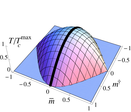
Figure 2: (Color online) Phase boundary in terms of the magnetization $\bar{m}\!=\!\mbox{$\frac{1}{2}$}(m_{1}+m_{2})$ and $m^{\dagger}\!=\!\mbox{$\frac{1}{2}$}(m_{1}-m_{2})$ in the symmetric case. Criticality occurs on the bold line. The surface represents the limit of the single-phase region. Below the surface the parameter $u$ sticks at zero.

Our result (90) and subsequent relations (91)-(93), describe the equation of state, i.e. the relations between the densities, $m_{1}$, $m_{2}$, or $\rho_{1}$ and $\rho_{2}$, and the fields, $h_{1}$, and $h_{2}$, or chemical potentials, $\mu_{1}$ and $\mu_{2}$, at temperature $T$ close to criticality. To reveal specific, characteristic features we consider, first, the phase boundary in terms of the sum and difference densities $\check{m}$ and $\check{m}^{\dagger}$. It follows from (90) that the phase boundary below and up to $T_{c}(\check{m}^{\dagger})$ is determined by the relation $u(t,\check{m},\check{m}^{\dagger})\!=\!0$. Figure 2 depicts the boundary in the space $(T,\bar{m},m^{\dagger})$ for a symmetric system, for which the critical locus was already derived in (81). Evidently, at fixed $m^{\dagger}$ and for $T<T_{c}(m^{\dagger})$ there is a composition gap $\Delta\bar{\rho}(T)\!=\!\bar{\rho}_{\alpha}-\bar{\rho}_{\beta}$, where $\alpha$ and $\beta$ label the two phases. This vanishes as $T\rightarrow T_{c}(m^{\dagger})$ and from the magnetic perspective is most readily expressed in terms of the spontaneous magnetization which is described by

$$\check{m}_{0}(T)\approx B|t|^{\beta}\quad\mbox{with $\beta\!=\!\mbox{$\frac{1}{2}$}$},$$ (99)

where $B\!=\!(c_{t}/c_{m})^{1/2}$. In fact the critical exponent $\beta\!=\!\mbox{$\frac{1}{2}$}$ represents the standard “universal” spherical model result!

As regards the other critical exponents of the general binary fluid model, our choice of the mixing parameters $\theta$, $\theta_{m}$ and $\theta_{h}$ at fixed $\check{m}^{\dagger}$ ensures that they basically match those of the corresponding single-component spherical models. This, of course, is in agreement with general considerations of the thermodynamics of multi-component fluids Griffiths and Wheeler (1970). Thus regarding the density correlation functions, the decomposition (49) shows that the dominant behavior of the density structure function near criticality is given by

$$S_{{\scriptscriptstyle NN}}(\mathbf{k};T,\boldsymbol{\rho})\approx 1/(u+k^{2}R_{c}^{2}+\ldots)\,,$$ (100)

where $R_{c}$ is a nonzero range parameter, while on the critical isochore, $\check{m}\!=\!\check{m}_{c}\!=\!0$, we have $u\sim t^{\gamma}$ as follows from (82). Hence, we find $S_{{\scriptscriptstyle NN}}(\mathbf{k}\!=\!\mathbf{0};T,\boldsymbol{\rho}_{c})\!\sim\!1/t^{\gamma}$ which is consistent with the definition of the critical exponent $\gamma$ via, say, light scattering experiments. At criticality, this result also implies $S_{{\scriptscriptstyle NN}}(\mathbf{k};T_{c},\rho_{c})\!\sim\!1/k^{2}$, which confirms the classical value $\eta\!=\!0$ of the critical point decay exponent.

Moreover, in leading order close to but above criticality one can establish the scaling form

$$S_{{\scriptscriptstyle NN}}(\mathbf{k};T,\rho_{c})\approx t^{-\gamma}X_{{\scriptscriptstyle NN}}[k\xi_{{\scriptscriptstyle N}}(T)],$$ (101)

where the density correlation length is $\xi_{{\scriptscriptstyle N}}(T)\!\approx\!\xi_{0}/t^{\nu}$ with critical exponent $\nu\!=\!\mbox{$\frac{1}{2}$}\gamma$ in accord with the general scaling relation $\gamma\!=\!(2-\eta)\nu$. The scaling function $X_{{\scriptscriptstyle NN}}(x)$ has the standard Ornstein-Zernike form $\varpropto\!1/(1+x^{2})$.

However, the equation of state in terms of $T$, $\check{m}$, and the field $\check{h}$ requires further examination. Thus, while the standard spherical model singularities embodied in (58) are evident, new features arise from the “demagnetization” term ${\mathfrak{n}}\check{m}$ on the left hand side of (90). To understand their significance, consider symmetric systems (i.e., with $\widehat{J}_{{\scriptstyle{11}}}\!=\!\widehat{J}_{{\scriptstyle{22}}}$), where (90) reduces to

$$\bar{h}\approx{\mathfrak{n}}\bar{m}+j_{0}p^{-\gamma}(c_{t}t+c_{m}\bar{m}^{2})^{\gamma},$$ (102)

while the demagnetization factor ${\mathfrak{n}}(\bar{m},m^{\dagger})$ is then given by (94) and vanishes only if $m^{\dagger}\!=\!0$. More generally, however, we note that ${\mathfrak{n}}(\check{m}\!=\!0,\check{m}^{\dagger})$ vanishes in asymmetric systems, only on the special two loci $\check{m}^{\dagger}\!=\!\pm\check{m}^{\dagger}_{s}$ where one finds

$$\check{m}^{\dagger^{{\scriptstyle{2}}}}_{s}=(1-\theta\theta_{m}^{2})^{2}w(\theta)/4\theta^{2}\theta_{m}^{4}c_{0}.$$ (103)

It now follows from (102) that the inverse thermodynamic susceptibility or partial compressibility, $1/\chi\equiv(\partial\bar{h}/\partial\bar{m})_{t}$, does not vanish at the critical point $t\!=\!0$, $\bar{m}_{c}\!=\!0$: see Figure 3. Consequently, the susceptibility does not diverge near criticality in the general case! The culprit is clearly the demagnetization effect, i.e., the term ${\mathfrak{n}}\bar{m}$ which arises both from the compositional asymmetry (when $\check{m}^{\dagger}\!\neq\!0$) reflecting the multicomponent nature of the binary fluid, and, from the underlying vectorial character of the order parameter: recall that spherical models correspond to the $n\rightarrow\infty$ limit of systems of vector-valued spins. Indeed, as we demonstrate in the next section, the origin of the demagnetization effect in spherical models can be understood directly in terms of vector spin models.

Figure 3: Schematic depiction of the equation of state at fixed $\check{m}^{\dagger}$ ($\neq 0$) in a symmetric system for temperatures above, at, and below criticality. In the latter case, the equation of state reduces to the linear demagnetization form $\bar{h}\!=\!{\mathfrak{n}}\bar{m}$ (dashed line) for $-\bar{m}_{0}\leq\bar{m}<\bar{m}_{0}$ (where $\bar{m}_{0}\sim t^{\beta}$) and $\bar{h}$ in the interval $(-\bar{h}_{0},\bar{h}_{0})$.

The nondivergence of the susceptibility/compressibility $\chi$ means that standard isothermal plots of the chemical potential (or, similarly, the pressure) vs. density or of magnetic field vs. magnetization near criticality take the form illustrated in Fig. 3 with, in general, a nonzero slope at $T\!=\!T_{c}$ fixed by the value, ${\mathfrak{n}}_{c}$, of the demagnetization coefficient. Note, in particular, that below $T_{c}$ what would in a standard fluid system be a constant isotherm of zero slope through the two-phase region — i.e., the interval set by the spontaneous magnetization, $m_{0}(T)$ — is now replaced by a straight line with the same fixed slope ${\mathfrak{n}}_{c}$ (at least close to $T_{c}$).

It is this fact that leads us to call this anomalous behavior, certainly unphysical in a fluid model, a “demagnetization effect”. To be more specific, in a real magnetic system with long-range dipole-dipole interactions, one must distinguish between the externally applied magnetic field $H_{{\textrm{ext}}}$, analogous here to $\bar{h}$ (or $\check{h}$), and the internal field, $H_{{\textrm{int}}}$, which is what is “seen” by individual atomic and molecular spins. The relation between these may be written

$$H_{{\textrm{int}}}=H_{{\textrm{ext}}}-NM,$$ (104)

where $M$, analogous here to $\bar{m}$ (or $\check{m}$) is the magnetization while $N$ is the demagnetization coefficient Starling (1941); Landau and Lifshitz (1960); Mattis (1965). More generally the fields $\mathbf{H}_{{\textrm{int}}}$ and $\mathbf{H}_{{\textrm{ext}}}$ are real-space vectors, as is $\mathbf{M}$, and the relation (104) can be used only when the system is in the form of an ellipsoid and directions parallel to the major axes are considered. (In the case of a sphere one has $N\!=\!4\pi/3$ Starling (1941); Landau and Lifshitz (1960); Mattis (1965).)

One might, in light of these considerations, ask if one should not, similarly, be able to introduce an “effective internal field”, $\check{h}_{{\textrm{int}}}\approx\check{h}_{{\textrm{ext}}}-{\mathfrak{n}}\check{m}$, that would play a natural thermodynamic role. However, on the one hand, given the implicit variation of ${\mathfrak{n}}(\check{m},\check{m}^{\dagger})$, this seems unlikely to be related to the basic thermodynamic parameters, $T$, $\mu_{\sigma}$, and $\rho_{\sigma}$, sufficiently directly to be of real value, and, on the other hand, the higher order terms in (90) indicate that the linear slope shown in Fig. 3 for the “two-phase” region, will become nonlinear outside the critical region.

Finally, as a further caution, another unphysical feature of the present multicomponent fluid models must be noted. Indeed, it enters even in single-component spherical models Fisher (2005); Fisher and Aqua ; Fisher (1992)! Specifically, whenever $\gamma\!>\!1$ and ${\mathfrak{n}}_{c}\!=\!0$ so that the susceptibility $\chi$ diverges to $\infty$ on approach to $T_{c}$ along the critical isochore, it also diverges when the phase boundary is approached below $T_{c}$. Even for ${\mathfrak{n}}_{c}\!\neq\!0$, a corresponding anomalous feature arises and is embodied in Fig. 3 where the slope of the isotherm below $T_{c}$ remains continuous through the phase boundaries (marked by open circles); but in realistic fluid models there would be breaks in the slope!

V Vector spin model analysis

To understand the origin of the demagnetization-like effects that enter the present multi-component spherical models, it is helpful to recognize that spherical models correspond precisely to the $n\!\rightarrow\!\infty$ limit of appropriate systems of $n$-component spins Stanley (1968). The vectorial character of the order parameter is thus a trademark of the model Fisher (2005); Fisher and Aqua , coupled here to asymmetry and multicomponent features. The ‘secret’ of the demagnetization effect appearing first in (90) can then be understood by regarding our binary-fluid spherical models as magnetic models with two classes of spins on separate sublattices, just as in (1)-(14), but now as fixed length vector spins, $\mathbf{s}_{\sigma}(\mathbf{R}^{\sigma}_{{i}})$ ($\sigma\!=\!1,2$), rather than scalar Ising spins as originally contemplated.

To obtain insight into the behavior of the model below $T_{c}$, we may use a simple mean-field approach by representing the overall sublattice magnetizations by two mean values, $\mathbf{m}_{1}$ and $\mathbf{m}_{2}$. The lengths of these magnetization vectors should ideally be taken as $m_{\sigma}^{0}(T)$, the spontaneous magnetizations (at fixed $T\!<\!T_{c}$); but it suffices here to consider the symmetric situation and so accept equal fixed lengths $|\mathbf{m}_{1}|\!=\!|\mathbf{m}_{2}|\!=\!1$.

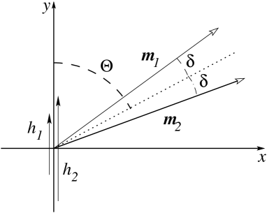
Figure 4: Vectorial representation of the two-species spherical model within a mean-field picture in which $\mathbf{m}_{1}$ and $\mathbf{m}_{2}$ are the two sublattice magnetization vectors that can rotate with respect to the direction, the $y$ axis, set by the parallel external fields, $\mathbf{h}_{1}$ and $\mathbf{h}_{2}$.

Then, in contrast to most realistic magnetic systems, it is imperative to allow for the imposition of two distinct external magnetic fields $\mathbf{h}_{1}$ and $\mathbf{h}_{2}$, corresponding, as fundamental for fluid models, to two distinct chemical potentials $\mu_{1}$ and $\mu_{2}$. However, for the “chemical interpretation”, we must take $\mathbf{h}_{1}$ parallel to $\mathbf{h}_{2}$ and may identify the preferred direction as the $y$ axis: see Fig. 4. The components $(\mathbf{m}_{1})_{y}$ and $(\mathbf{m}_{2})_{y}$ then correspond to the densities $m_{1}$ and $m_{2}$ in our previous analysis, while

$$\bar{h}\!=\!\mbox{$\frac{1}{2}$}(h_{1}+h_{2})\quad\mbox{with}\quad h_{\sigma}\!=\!(\mathbf{h}_{\sigma})_{y}$$ (105)

describes the external field/chemical potential. On the other hand, $h^{\dagger}\!=\!\mbox{$\frac{1}{2}$}(h_{1}-h_{2})$ characterizes the compositional asymmetry of the system (even when the two species, here the magnetic sublattices, are symmetrically related): that asymmetry is at the heart of the matter. As regards the vector-spin dimensionality, however, it suffices to allow for only one more dimension and so, regard the $\mathbf{m}_{\sigma}$ as XY or O$(2)$ order parameters.

Finally, beyond the symmetric intrasublattice ferromagnetic couplings (that lead to the spontaneous magnetizations), we allow for the intersublattice interactions by a coupling constant $j\!>\!0$ (analogous to $j_{0}$ above). Thus we take the essential part of the mean-field free energy to be

$$\mathcal{F}(\bar{h};h^{\dagger};\mathbf{m}_{1},\mathbf{m}_{2})=-\mathbf{h}_{1}\mathbf{\cdot}\mathbf{m}_{1}-\mathbf{h}_{2}\mathbf{\cdot}\mathbf{m}_{2}-j\mathbf{m}_{1}\mathbf{\cdot}\mathbf{m}_{2}.$$ (106)

Here the external field $\bar{h}$ is the control variable while $h^{\dagger}$ is fixed and, as usual, $\mathcal{F}$ is to be minimized with respect to $\mathbf{m}_{1}$ and $\mathbf{m}_{2}$.

Let us, as in Fig. 4, introduce the mean tilt angle $\Theta$ between the $y$-axis and $\bar{\mathbf{m}}\!=\!\mbox{$\frac{1}{2}$}(\mathbf{m}_{1}+\mathbf{m}_{2})$ and the splitting or separation angle $\delta$, between the $\mathbf{m}_{\sigma}$ and the $\bar{\mathbf{m}}$. For simplicity we suppose that $\delta$ is small (which requires $|h^{\dagger}|\ll j$); then minimization on $\delta$ yields

$$\mathcal{F}_{\min}(\Theta)=-j-2\bar{h}\cos\Theta-\frac{2h^{\dagger^{{\scriptstyle{2}}}}\sin^{2}\Theta}{2j+\bar{h}\cos\Theta}+{\mathcal{O}}(h^{\dagger^{{\scriptstyle{2}}}}/j^{2}).$$ (107)

Consider, first, the fully symmetric case in which $h^{\dagger}\!=\!0$ (and $\delta_{\min}\!=\!0$). Minimizing this expression on $\Theta$ then gives $\Theta_{\min}\!=\!0$ for $\bar{h}\!=\!0$ but $\Theta_{\min}\!=\!\pi$ for $\bar{h}\!<\!0$. This evidently corresponds to the usual ferromagnetic situation in which (neglecting dipolar interactions and demagnetization effects) the magnetization $\bar{\mathbf{m}}$ switches abruptly from $\bar{m}\equiv(\bar{\mathbf{m}}_{\sigma})_{y}\!=\!-1$ to $+1$ as the field $\bar{h}$ passes through zero.

On the other hand when $h^{\dagger}\!\neq\!0$ the minimizing value of $\Theta$ assumes a nontrivial value for $\bar{h}$ between the limits $\pm\bar{h}_{0}$ given by

$$\bar{h}_{0}=j\left(\sqrt{1+h^{\dagger^{{\scriptstyle{2}}}}/j^{2}}-1\right)\approx\mbox{$\frac{1}{2}$}h^{\dagger^{{\scriptstyle{2}}}}/j,$$ (108)

up to corrections of relative order $(h^{\dagger}/j)^{2}$. As a consequence, the magnetization $\bar{m}(\bar{h})$ no longer jumps discontinuously at $\bar{h}\!=\!0$ from $\bar{m}\!=\!-1$ to $\bar{m}\!=\!+1$ but rather varies continuously and almost linearly over the interval $-\bar{h}_{0}\!\leq\!\bar{h}\!<\!\bar{h}_{0}$ according to

$$\bar{m}(\bar{h})\simeq\frac{\bar{h}}{\bar{h}_{0}}\left[1-\mbox{$\frac{3}{8}$}(h^{\dagger}/j)^{2}\right]/\left[1-\mbox{$\frac{3}{8}$}(h^{\dagger}/j)^{2}(\bar{h}/\bar{h}_{0})^{2}\right].$$ (109)

More explicitly to leading order in $(h^{\dagger}/j)^{2}$ one finds for $|\bar{h}|\!<\!\bar{h}_{0}$,

$$\bar{m}=\cos\Theta_{\min}=\frac{2j}{\bar{h}}\left[\sqrt{\frac{1-\bar{h}^{2}/4j^{2}}{1-2\bar{h}^{2}/h^{\dagger^{{\scriptstyle{2}}}}}}-1\right]\,,$$ (110)

while for $|\bar{h}|\!>\!\bar{h}_{0}$ one has $\cos\Theta\!=\!\textrm{sgn}\{\bar{h}\}$.

In words, for an external field $\bar{h}$ not too large compared to the square of the asymmetric field $h^{\dagger}$, the spins cant themselves in a direction $\Theta_{\min}\neq 0$, with, indeed, $\Theta_{\min}\!=\!\pi/2$ when $\bar{h}\!=\!0$! This minimizing behavior of vector spins is clearly the origin of the seeming demagnetization effect and explains our result for the spherical model. Indeed, near the origin, for $\bar{h}/\bar{h}_{0}\rightarrow 0$, we find $\cos\Theta_{\min}\approx 2\bar{h}j/h^{\dagger^{{\scriptstyle{2}}}}$ which leads to a nondivergent susceptibility of magnitude

$$\chi\!=\!\left(\partial\bar{m}/\partial\bar{h}\right)_{T,\bar{h}=0}=2j/h^{\dagger^{{\scriptstyle{2}}}}.$$ (111)

Thus, as the spherical model itself, the asymmetry of the spin model, coupled to the vectorial character of the order parameter, leads to a non-vanishing inverse susceptibility near criticality in the general case. Note also that, as in the spherical model, the divergence of $\chi$ re-emerges in the symmetric case when $h^{\dagger}\!=\!0$. Finally, the nonlinear terms in $\bar{h}$ implied by (109) show that one cannot hope to find a simple demagnetization description as in Starling (1941); Landau and Lifshitz (1960); Mattis (1965).

VI Conclusions

We have introduced multicomponent generalizations of the standard spherical model that embody lattice-gas hard cores for many-species fluids by using interlaced sublattices. Taking into account a spherical constraint for each distinct species, we have obtained exact expressions for the free energy and pair correlation functions in the general case, in terms of the basic Fourier space interaction matrix. We have then focused on binary fluids where the diagonalization of $2\!\times\!2$ matrices leads to relatively simple results for the physical properties of the system. We find that density and (for ionic fluids) charge correlation functions can be decomposed naturally in terms of two eigenmodes. This formulation, which could well have broader validity, has dramatic consequence for charged fluids as we expound elsewhere Fisher (2005); Fisher and Aqua ; Aqua and Fisher (2004a, b, ).

The present article considers fluids where, in addition to hard cores, only short-range overall attractive interactions are present. We show that with an appropriate choice of variables (in the form of linear combinations of the mean magnetizations/densities or external fields/chemical potentials for the two species), the usual critical properties of single-component spherical models can be uncovered in accord with general thermodynamic arguments for multicomponent solutions. Specifically, as the relative composition of the system varies, criticality is realized on a well defined locus in the full phase diagram.

However, an unexpected and intrinsically unphysical “pseudodemagnetization phenomenon” arises that, except on certain submanifolds, prevents the usual divergence of the thermodynamic susceptibilities/compressibilities at criticality. This feature, undesirable for model fluids, is found to be a consequence of an interplay between species and compositional asymmetry and the multidimensional characteristics represented by the hidden vectorial character of the order parameter in spherical models. The behavior can, indeed, be understood via a simple mean-field description of a corresponding XY spin model. Despite this artificial aspect, requiring caution in interpreting results, further aspects of the multicomponent spherical models seem worth pursuing: on the one hand, ternary fluid models with, say, positive and negative ions in solutions of neutral molecules, could be instructive; on the other hand, magnetic systems with different types of ions could reveal interesting behavior.

Appendix A Location of singularities

In this appendix, we locate the singularities of the binary spherical model for the generic case of short-range interactions. The singularities derive from the vanishing of $\Lambda_{-}(\mathbf{k};\boldsymbol{\lambda})$ and we obtain sufficient conditions to ensure that they arise only when $\mathbf{k}\!=\!\mathbf{0}$.

A.1 Vicinity of the origin

We first consider the small-$\mathbf{k}$ behavior of $\Lambda_{-}(\mathbf{k};\boldsymbol{\lambda})$. Owing to the second condition (71), the range $R_{{\scriptstyle{12}}}$ defined in (70) satisfies $R_{{\scriptstyle{12}}}^{2}\!>\!0$. Note also the relations $\Delta\bar{J}(\mathbf{k})\!\approx\!j_{0}\bar{R}^{2}k^{2}$ and $\Delta J^{\dagger}(\mathbf{k})\!\approx\!j_{0}{R^{\dagger}}^{2}k^{2}$, where $\bar{R}$ and $R^{\dagger}$ are characteristic ranges. At leading order in $k$ we then have

$$\frac{\Lambda_{-}(\mathbf{k};\boldsymbol{\lambda})-\Lambda_{-}(\mathbf{0};\boldsymbol{\lambda})}{j_{0}k^{2}}=\bar{R}^{2}+\frac{j_{0}R_{{\scriptstyle{12}}}^{2}-\lambda^{\dagger}{R^{\dagger}}^{2}}{\sqrt{\lambda^{\dagger^{{\scriptstyle{2}}}}+{j_{0}}^{2}}}+\cdots,$$ (112)

which will be valid in a domain $|\mathbf{k}|\leq k_{m}\!>\!0$. From the third condition (71) we find $\bar{R}^{2}\!>\!0$ and if, recalling the definition (35b) of $\Delta J^{\dagger}$, we accept the further condition

$$|{R^{\dagger}}^{2}|=\lim_{k\rightarrow 0}\Delta J^{\dagger}(\mathbf{k})/j_{0}k^{2}\leq\bar{R}^{2},$$ (113)

we are assured that $\mathbf{k}\!=\!\mathbf{0}$ is indeed the minimum of $\Lambda_{-}(\mathbf{k};\boldsymbol{\lambda})$ when $k\leq k_{m}$.

A.2 Remainder of the Brillouin zone

Consider now the subdomain $\mathcal{B}^{\prime}$ of the Brillouin zone $\mathcal{B}$, consisting of all vectors $\mathbf{k}$ outside the origin domain $|\mathbf{k}|\leq k_{m}$. In the symmetric case when $\Delta J^{\dagger}\!=\!0$ (marked by superscripts sym), the second condition (71) leads to $|\widehat{J}_{{\scriptstyle{12}}}(\mathbf{k})|\!<\!j_{0}$ so that

$$\Delta\Lambda_{-}^{{\textrm{sym}}}\equiv\Lambda_{-}^{{\textrm{sym}}}(\mathbf{k};\boldsymbol{\lambda})-\Lambda_{-}^{{\textrm{sym}}}(\mathbf{0};\boldsymbol{\lambda})>\Delta\bar{J}(\mathbf{k})\,.$$ (114)

But, according to the last member of (71), there exists a $\delta\Lambda_{-}^{{\textrm{sym}}}$ such that

$$\Delta\Lambda_{-}^{{\textrm{sym}}}(\mathbf{k};\boldsymbol{\lambda})\geq\delta\Lambda_{-}^{{\textrm{sym}}}>0\,,\,\,\textrm{for $\mathbf{k}\in\mathcal{B}^{\prime}$}\,.$$ (115)

In the general case where $\Delta J^{\dagger}$ is arbitrary, we may write

$$\Lambda_{-}(\mathbf{k};\boldsymbol{\lambda})-\Lambda_{-}(\mathbf{0};\boldsymbol{\lambda})=\Delta\Lambda_{-}^{{\textrm{sym}}}(\mathbf{k};\boldsymbol{\lambda})+\delta\Lambda_{-}[\Delta J^{\dagger}(\mathbf{k})]\,,$$ (116)

where from (36) we define

$$\delta\Lambda_{-}[\Delta J^{\dagger}(\mathbf{k})]=\sqrt{\lambda^{\dagger^{{\scriptstyle{2}}}}+\mbox{$\frac{1}{4}$}\widehat{J}_{{\scriptstyle{12}}}^{2}(\mathbf{k})}-\sqrt{[\lambda^{\dagger}+\Delta J^{\dagger}(\mathbf{k})]^{2}+\mbox{$\frac{1}{4}$}\widehat{J}_{{\scriptstyle{12}}}^{2}(\mathbf{k})}\,.$$ (117)

Then, noting that $|\partial(\delta\Lambda_{-})/\partial\Delta J^{\dagger}(\mathbf{k})|\leq 1$ and $\Delta J^{\dagger}(0)\!=\!0$, we see that $|\delta\Lambda_{-}[\Delta J^{\dagger}(\mathbf{k})]|\leq|\Delta J^{\dagger}(\mathbf{k})|$. Hence, accepting the further condition

$$\max_{\mathbf{k}\in\mathcal{B}^{\prime}}\left[|\Delta J^{\dagger}(\mathbf{k})|\right]<\delta\Lambda_{-}^{{\textrm{sym}}}\,,$$ (118)

which means that the asymmetry is not too strong, one concludes that $\Lambda_{-}(\mathbf{k};\boldsymbol{\lambda})\!>\!\Lambda_{-}(\mathbf{0};\boldsymbol{\lambda})$ for all $\mathbf{k}$ in $\mathcal{B}^{\prime}$.

References

• Weingärtner and Schröer (2001) H. Weingärtner and W. Schröer, Adv. Chem. Phys. 116, 1 (2001).
• Berlin and Kac (1952) T. H. Berlin and M. Kac, Phys. Rev. 86, 821 (1952).
• Lewis and Wannier (1952) H. W. Lewis and G. H. Wannier, Phys. Rev. 88, 682 (1952).
• Fisher (2005) M. E. Fisher, in Current Topics in Physics, edited by R. A. Barrio and K. K. Kaski (U.K.: Imperial College Press, 2005), chap. 1, p. 1.
• (5) M. E. Fisher and J.-N. Aqua, Rev. Mod. Phys., to appear.
• Joyce (1972) G. S. Joyce, in Phase Transitions and Critical Phenomena, edited by C. Domb and M. S. Green (Academic, New-York, 1972), vol. 2, p. 375.
• Barber and Fisher (1973) M. N. Barber and M. E. Fisher, Ann. Phys. (N.Y.) 77, 1 (1973).
• Kosterlitz et al. (1976) J. M. Kosterlitz, D. J. Thouless, and R. C. Jones, Phys. Rev. Lett. 36, 1217 (1976).
• Tu and Weichman (1994) Y. Tu and P. B. Weichman, Phys. Rev. Lett. 73, 6 (1994); T. M. Nieuwenhuizen. Phys. Rev. Lett. 74, 4293 (1995); T. Vojta and M. Schreiber, Phys. Rev. B 53, 8211 (1996).
• Paessens and Henkel (2003) M. Paessens and M. Henkel, EuroPhys. Lett. 62, 664 (2003).
• Gordon and Fischer (2004) A. Gordon and B. Fischer, Opt. Lett. 29, 1022 (2004).
• Chamati and Dantchev (2004) H. Chamati and D. M. Dantchev, Phys. Rev. E 70, 066106 (2004).
• Stanley (1968) H. E. Stanley, Phys. Rev. 176, 718 (1968).
• Smith (1988) E. R. Smith, J. Stat. Phys. 50, 813 (1988).
• Aqua and Fisher (2004a) J.-N. Aqua and M. E. Fisher, Phys. Rev. Lett. 92, 135702 (2004a).
• Aqua and Fisher (2004b) J.-N. Aqua and M. E. Fisher, J. Phys. A: Math. and Gen. 37, L241 (2004b).
• (17) J.-N. Aqua and M. E. Fisher, submitted for publication.
• Fisher (1992) M. E. Fisher, J. Chem. Phys. 96, 3352 (1992).
• See et al. (1952) See, e.g., T. D. Lee, and C. N. Yang, Phys. Rev. 87, 410 (1952).
• See et al. (1978) See also S. Sarbach, and M. E. Fisher, Phys. Rev. B 18, 2350 (1978).
• Onsager (1944) L. Onsager, Phys. Rev. 65, 117 (1944).
• Barbosa and Fisher (1991) M. C. Barbosa and M. E. Fisher, Phys. Rev. B. 43, 10635 (1991).
• Griffiths and Wheeler (1970) R. B. Griffiths and J. C. Wheeler, Phys. Rev. A 2, 1047 (1970).
• Starling (1941) S. G. Starling, Electricity and Magnetism (Longman, Green & Co., Seventh Edn., London, 1941), chap. IX, pp. 271–3.
• Landau and Lifshitz (1960) L. D. Landau and E. M. Lifshitz, Electrodynamics of Continuous Media (Pergamon Press, Oxford, 1960), vol. 8 of Course of Theoretical Physics, secs. 8, 27, 42.
• Mattis (1965) D. C. Mattis, The Theory of Magnetism (Harper and Row, New York, 1965) pp. 123–4, 133–6.