UNIVERSIDAD DE CHILE
FACULTAD DE CIENCIAS FÍSICAS Y MATEMÁTICAS
DEPARTAMENTO DE ASTRONOMÍA

DETERMINACIÓN DE LA DISTANCIA A 12 SUPERNOVAS DE TIPO II MEDIANTE EL MÉTODO DE LA FOTÓSFERA EN EXPANSIÓN

TESIS PARA OPTAR AL GRADO DE MAGÍSTER EN
CIENCIAS, MENCIÓN ASTRONOMÍA

MATÍAS IGNACIO JONES FERNÁNDEZ

DEDICATION

A mi familia, Padre, Madre y hermanos                                                                                            y a mi amada Carolina

RESUMEN

Hemos usado fotometría y espectroscopía temprana de 12 Supernovas de Tipo II plateau (SNs IIP) para derivar sus distancias mediante el Método de la Fotósfera en Expansión (EPM). Hemos realizado este estudio usando dos sets de modelos de atmósfera de Supernovas de Tipo II (SNs II), obtenidos de Eastman et al. (1996) y Dessart & Hillier (2005b), tres sets de filtros ({BV},{BVI},{VI}) y dos métodos para la determinación de la extinción en la galaxia huésped, con lo cual hemos construido 12 diagramas de Hubble. Usando el set de filtros $\{VI\}$ y los modelos de Dessart & Hillier (2005b) hemos obtenido una disperisíon en el diagrama de Hubble de $\sigma_{\mu}$ = 0.32 mag y su correspondiente constante de Hubble de $H_{0}$ = 52.4 $\pm$ 4.3 $km$ $s^{-1}$ $Mpc^{-1}$. Además aplicamos el EPM a la SN IIP SN 1999em. Con el set de filtros $\{VI\}$ y los modelos de Dessart & Hillier (2005b) hemos derivado una distancia a ésta de 13.9 $\pm$ 1.4 Mpc, lo cual concuerda con la distancia de Cefeida de 11.7 $\pm$ 1.0 Mpc a la galaxia huésped de ésta Supernova (NGC 1637).

List of Tables

2.1       Telescopes and instruments   . . . . . . . . . . . . . . . . . . . . . . . . . . . . . .     66
2.1       Telescopes and instruments (continued)   . . . . . . . . . . . . . . . . . . . . . . .     67
2.2       SNe redshifts   . . . . . . . . . . . . . . . . . . . . . . . . . . . . . . . . . . . . . . .     68

3.1       Dilution factors coefficients   . . . . . . . . . . . . . . . . . . . . . . . . . . . . . .     69
3.2       Spectroscopic velocities   . . . . . . . . . . . . . . . . . . . . . . . . . . . . . . . . .     70
3.2       Spectroscopic velocities (continued)   . . . . . . . . . . . . . . . . . . . . . . . . .     71
3.2       Spectroscopic velocities (continued)   . . . . . . . . . . . . . . . . . . . . . . . . .     72
3.2       Spectroscopic velocities (continued)   . . . . . . . . . . . . . . . . . . . . . . . . .     73
3.2       Spectroscopic velocities (continued)   . . . . . . . . . . . . . . . . . . . . . . . . .     74
3.2       Spectroscopic velocities (continued)   . . . . . . . . . . . . . . . . . . . . . . . . .     75
3.2       Spectroscopic velocities (continued)   . . . . . . . . . . . . . . . . . . . . . . . . .     76
3.2       Spectroscopic velocities (continued)   . . . . . . . . . . . . . . . . . . . . . . . . .     77
3.3       Photospheric velocity conversion coefficients   . . . . . . . . . . . . . . . . . . . .     78
3.4       Host galaxy ad Galactic extinction   . . . . . . . . . . . . . . . . . . . . . . . . . .     79
3.5       EPM distances   . . . . . . . . . . . . . . . . . . . . . . . . . . . . . . . . . . . . . .     80
3.6       Error sources   . . . . . . . . . . . . . . . . . . . . . . . . . . . . . . . . . . . . . . .     81
3.7       EPM quantities derived for SN 1992ba   . . . . . . . . . . . . . . . . . . . . . . . .     82
3.8       EPM quantities derived for SN 1999br   . . . . . . . . . . . . . . . . . . . . . . . .     83
3.9       EPM quantities derived for SN 1999em   . . . . . . . . . . . . . . . . . . . . . . .     84
3.9       EPM quantities derived for SN 1999em (continued)   . . . . . . . . . . . . . . . .     85
3.10     EPM quantities derived for SN 1999gi   . . . . . . . . . . . . . . . . . . . . . . . .     86
3.11     EPM quantities derived for SN 2002gw   . . . . . . . . . . . . . . . . . . . . . . .     87
3.12     EPM quantities derived for SN 2003T   . . . . . . . . . . . . . . . . . . . . . . . .     88
3.13     EPM quantities derived for SN 2003bl   . . . . . . . . . . . . . . . . . . . . . . . .     89
3.14     EPM quantities derived for SN 2003bn   . . . . . . . . . . . . . . . . . . . . . . . .     90
3.15     EPM quantities derived for SN 2003ef   . . . . . . . . . . . . . . . . . . . . . . . .     91
3.16     EPM quantities derived for SN 2003hl   . . . . . . . . . . . . . . . . . . . . . . . .     92
3.17     EPM quantities derived for SN 2003hn   . . . . . . . . . . . . . . . . . . . . . . . .     93
3.18     EPM quantities derived for SN 2003iq   . . . . . . . . . . . . . . . . . . . . . . . .     94

4.1       Summary of $H_{0}$ values   . . . . . . . . . . . . . . . . . . . . . . . . . . . . . . . . .     95
4.2       Summary of dispersions in the Hubble diagrams   . . . . . . . . . . . . . . . . . . . .     96

List of Figures

2.1       Light curves (part 1)   . . . . . . . . . . . . . . . . . . . . . . . . . . . . . . . . . .     35
2.2       Light curves (part 2)   . . . . . . . . . . . . . . . . . . . . . . . . . . . . . . . . . .     36
2.3       Light curves (part 3)   . . . . . . . . . . . . . . . . . . . . . . . . . . . . . . . . . .     37

3.1       Dilution factors   . . . . . . . . . . . . . . . . . . . . . . . . . . . . . . . . . . . . . .     38
3.2       Line velocity evolution (part 1)   . . . . . . . . . . . . . . . . . . . . . . . . . . . .     39
3.3       Line velocity evolution (part 2)   . . . . . . . . . . . . . . . . . . . . . . . . . . . .     40
3.4       Line velocity evolution (part 3)   . . . . . . . . . . . . . . . . . . . . . . . . . . . .     41
3.5       Photospheric velocity conversion   . . . . . . . . . . . . . . . . . . . . . . . . . . .     42
3.6       Ratio between the $H_{\alpha}$ and $H_{\beta}$ velocity   . . . . . . . . . . . . . . . . . . . . . . . .     43
3.7       Comparison between the DES and OLI reddening   . . . . . . . . . . . . . . . . .     44
3.8       Full EPM solution for SN 1999em   . . . . . . . . . . . . . . . . . . . . . . . . . . .     45
3.9       EPM solution for SN 1992ba   . . . . . . . . . . . . . . . . . . . . . . . . . . . . . .     46
3.10     EPM solution for SN 1999br   . . . . . . . . . . . . . . . . . . . . . . . . . . . . . .     47
3.11     EPM solution for SN 1999em   . . . . . . . . . . . . . . . . . . . . . . . . . . . . .     48
3.12     EPM solution for SN 1999gi   . . . . . . . . . . . . . . . . . . . . . . . . . . . . . .     49
3.13     EPM solution for SN 2002gw   . . . . . . . . . . . . . . . . . . . . . . . . . . . . . .     50
3.14     EPM solution for SN 2003T   . . . . . . . . . . . . . . . . . . . . . . . . . . . . . .     51
3.15     EPM solution for SN 2003bl   . . . . . . . . . . . . . . . . . . . . . . . . . . . . . .     52
3.16     EPM solution for SN 2003bn   . . . . . . . . . . . . . . . . . . . . . . . . . . . . . .     53
3.17     EPM solution for SN 2003ef   . . . . . . . . . . . . . . . . . . . . . . . . . . . . . .     54
3.18     EPM solution for SN 2003hl   . . . . . . . . . . . . . . . . . . . . . . . . . . . . . .     55
3.19     EPM solution for SN 2003hn   . . . . . . . . . . . . . . . . . . . . . . . . . . . . . .     56
3.20     EPM solution for SN 2003iq   . . . . . . . . . . . . . . . . . . . . . . . . . . . . . .     57

4.1       EPM distances as a function of the host galaxy extinction   . . . . . . . . . . . .     58
4.2       Hubble diagrams using the $\{BV\}$ filter subset and OLI   . . . . . . . . . . . . . .     59
4.3       Hubble diagrams using the $\{BVI\}$ filter subset and OLI   . . . . . . . . . . . . .     60
4.4       Hubble diagrams using the $\{VI\}$ filter subset and OLI   . . . . . . . . . . . . . .     61
4.5       Hubble diagrams using the $\{BV\}$ filter subset and DES   . . . . . . . . . . . . .     62
4.6       Hubble diagrams using the $\{BVI\}$ filter subset and DES   . . . . . . . . . . . . .     63
4.7       Hubble diagrams using the $\{VI\}$ filter subset and DES   . . . . . . . . . . . . . .     64
4.8       Corrected E96 and D05 distances   . . . . . . . . . . . . . . . . . . . . . . . . . . .     65

ABSTRACT

We used early time photometry and spectroscopy of 12 Type II plateau Supernovae (SNe IIP) to derive their distances using the Expanding Photosphere Method (EPM). We performed this study using two sets of Type II supernovae (SNe II) atmosphere models from Eastman et al. (1996) and Dessart & Hillier (2005b), three filter subsets ({BV},{BVI},{VI}) and two methods for the host galaxy extinctions, which led to 12 Hubble diagrams. Using the $\{VI\}$ filter subset and the Dessart & Hillier (2005b) models we obtained a dispersion in the Hubble diagram of $\sigma_{\mu}$ = 0.32 mag and a Hubble constant of $H_{0}$ = 52.4 $\pm$ 4.3 $km$ $s^{-1}$ $Mpc^{-1}$. We also applied the EPM analysis to the well-observed SN IIP SN 1999em. With the $\{VI\}$ filter subset and the Dessart & Hillier (2005b) models we derived a distance of 13.9 $\pm$ 1.4 Mpc, which is in agreement with the Cepheid distance of 11.7 $\pm$ 1.0 Mpc to the SN 1999em host galaxy (NGC 1637).

1 Introduction

Type II supernovae (SNe II) are believed to be produced by the gravitational collapse of massive stars ($M$ $>$ $8M_{\sun}$), that at the moment of the explosion have most of their hydrogen envelope intact. The energy released in the explosion is typically $10^{53}$ erg (mainly in the form of neutrinos), and the luminosity of the SN during the first few months after explosion can be comparable to the total luminosity of its host galaxy. These objects have been classified based on their light curves into Type IIP (plateau) and Type IIL (linear) (Patat et al., 1994). The former present a nearly constant luminosity during the photospheric phase ($\sim$ 100 days after explosion), while the latter show a slow decline in luminosity during that phase. However, there are some SN II events, such as the SN 1987A, that show peculiar photometric properties. Also, further studies of SNe II spectra, have revealed the existence of a new subclass, characterized by the presence of narrow spectral lines, called SNe IIn.
Due to their high intrinsic luminosities, SNe II have great potential as extragalactic distance indicators. To date, several methods have been proposed to derive distances to SNe II, but two are the most commonly used: the Expanding Photosphere Method (EPM) (Kirshner & Kwan, 1974) and the Standardized Candle Method (SCM) (Hamuy & Pinto, 2002). The former is a geometrical technique that relates the physical radius and the angular radius of a SN in order to derive its distance, and has been applied to several SNe to derive the Hubble constant (Schmidt et al., 1992). The EPM is independent of the extragalactic distance ladder, and therefore does not need any external calibration. The SCM, is based on the observational relation between expansion velocity and luminosity of the SNe. Recently, this method has been applied to a sample of high redshift SNe (Nugent et al., 2006). Other methods have been used also to determine distances to SNe II such as the Spectral-fitting Expanding Atmosphere Method (SEAM) (Baron et al., 2004) or the Plateau-Tail relation proposed by Nadyozhin (2003).
In this work we apply the EPM using early spectroscopy and photometry of 12 SNe IIP in order to derive their distances. We apply the method using two sets of SNe II atmospheres models, from Eastman et al. (1996) and Dessart & Hillier (2005a), three filter subsets ($\{BV\},\{BVI\},\{VI\}$) and two methods for the host galaxy extinctions, which leads to 12 Hubble diagrams. This work is divided as follows: $\S$ 2 describes the photometric and spectroscopic observations. In $\S$ 3 is presented the Expanding Photosphere Method and the individual EPM analysis of 12 SNe IIP. In $\S$ 4.1 are described external comparisons to other methods and previous EPM analysis, in $\S$ 4.2 are discussed the error analysis and the effect of reddening in the EPM distances. In $\S$ 4.3 are shown 12 Hubble diagrams and the corresponding Hubble constants. In $\S$ 4.4 we propose an external calibration for the EPM. Finally, the conclusions are summarized in $\S$ 5.

2 Observations

In this work we use photometry and spectroscopy from four SN followup programs: the Cerro Tololo SN program (1986-1996), the Calán/Tololo survey (CT; 1990-1993), the Supernovae Optical and Infrared Survey (SOIRS; 1999-2000) and the Carnegie Type II Supernova Program (CATS; 2002-2003). During these programs optical (and some IR) photometry and spectroscopy were obtained for nearly 100 SNe, 51 of which belong to the Type II class. All of the optical data have already been reduced and they are in due course for publication (Hamuy et al., 2008). We also complemented our dataset with some spectroscopic observations from other authors.

2.1 Photometry

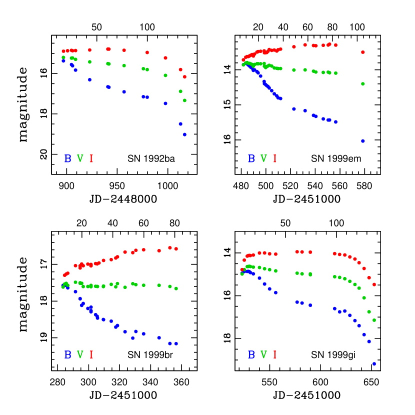
Figure 1: Optical light curves of four SNe during the first $\sim$ 120 days of their evolution. In the top of each panel is shown the date since the EPM explosion time derived using the D05 models (see Table 7).  

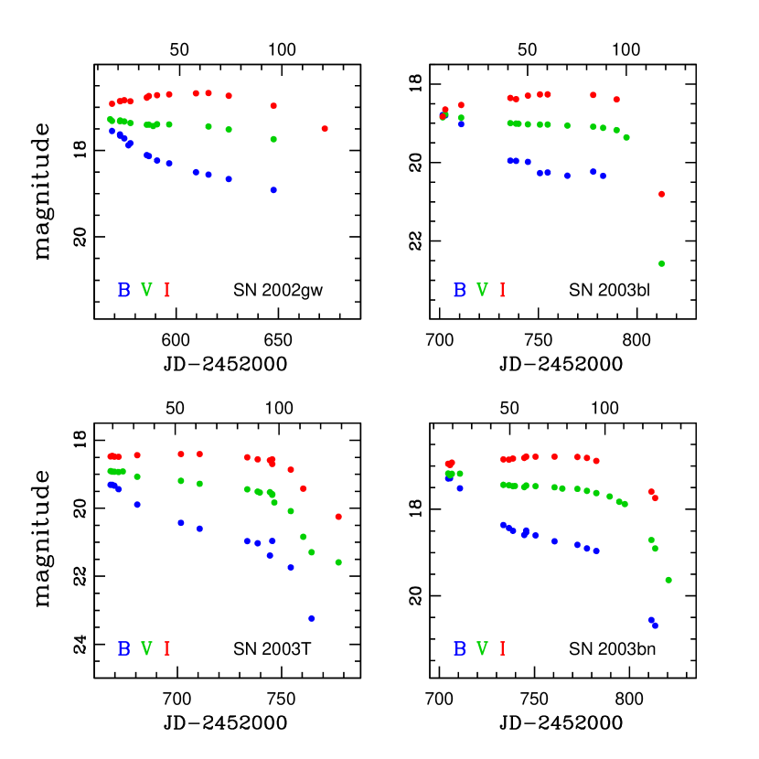
Figure 2: Optical light curves of four SNe during the first $\sim$ 120 days of their evolution. In the top of each panel is shown the date since the EPM explosion time derived using the D05 models (see Table 7).  

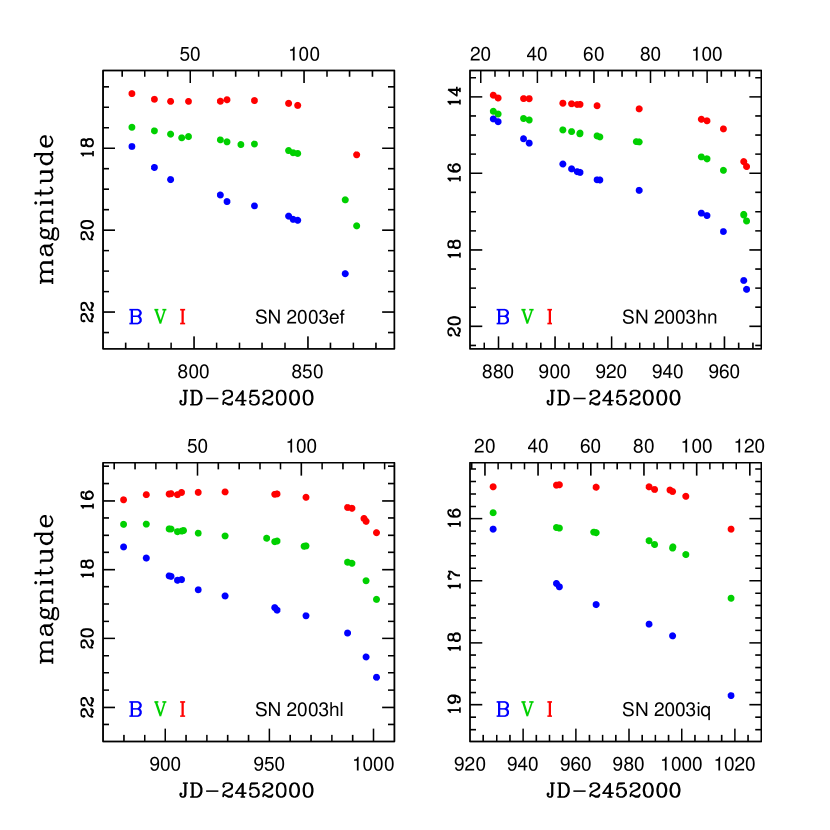
Figure 3: Optical light curves of four SNe during the first $\sim$ 120 days of their evolution. In the top of each panel is shown the date since the EPM explosion time derived using the D05 models (see Table 7).  

The observations were made with telescopes from four different observatories: the Cerro Tololo Inter-American Observatory (CTIO), the Las Campanas Observatory (LCO), the European Southern Observatory (ESO) in La Silla and the Steward Observatory (S0). Several telescopes and instruments were used to obtain the photometry as shown in Table 1. In all cases CCD detectors and standard Johnson-Kron-Cousins UBVRIZ filters (Johnson et al., 1966; Cousins, 1971) were employed. For a small subset of SNe observations in the JHK filters were also obtained. The data reductions were performed using IRAF according to the procedure described in Hamuy et al. (2008).
The optical light curves of all the SNe used in this work are shown in Figures 1-3 which clearly reveal the plateau nature of all these events.

2.2 Spectroscopy

Low resolution (R $\sim$ 1000) optical spectra (wavelength range $\sim$ 3200 - 10000 Å) were taken for each SN at various epochs using telescopes and instruments from four different observatories. Table 1 lists all the telescopes and instruments used for the spectroscopy. Most of the time the spectra were taken orienting the slit along the paralactic angle. The wavelength calibration was performed using comparison lamp spectra taken at the same position of each SN. The flux calibration was done via observations of flux standards stars (Hamuy et al., 1992, 1994). For more details on the observational procedures see Hamuy et al. (2008).
The spectra were taken to the rest frame using the heliocentric redshifts given in Table 2 in order to measure the SN ejecta velocities. In seven cases we were able to measure the redshifts from narrow emission lines of HII regions at the SN position (see Table 2). Also, in one case (SN 1999em) we adopted the value from Leonard et al. (2002) which corresponds to the redshift measured at the SN position. In four cases, we were unable to extract this information from our data and we had to rely on redshifts of the host galaxy centers. The latter does not take into account the rotation velocities of the host galaxies, which are typically $v\sim 200$ $km$ $s^{-1}$.

2.3 Sample of SNe used in this work

51 SNe II were observed in the surveys described above. From this sample, only 11 SNe comply with the EPM requirements, which are: 1) the optical SN light curve ($V$ and the $I$ bands) must show a nearly constant luminosity during the photospheric phase, i.e, the SN must belong to the SNe IIP class (see Figures 1-3); 2) the SN must to have early time photometry; 3) the SN must to have at least three early spectroscopic observations. The need for all of these requirements is discussed in $\S$ 3.6. To the sample of 11 SNe we added the SN IIP 1999gi, which has extensive photometry and spectroscopy published by Leonard et al. (2002b).

3 The Expanding Photosphere Method

3.1 Basic ideas of the EPM

The EPM is a geometrical technique that relates an angular size and a physical size of a SN, in order to derive its distance. Although the angular radius $\theta$ of a SN cannot be resolved spatially, it can be derived assuming a spherically symmetric expanding photosphere (reasonable assumption for SNe IIP, as discussed by Leonard et al. (2001)) that radiates as a black body “diluted” by a factor $\zeta^{2}$, i.e,

$$\theta=\frac{R}{D}=\sqrt{\frac{(1+z)f_{\lambda}}{{\pi}{\zeta_{{\lambda}^{{}^{\prime}}}^{2}}B_{{\lambda}^{{}^{\prime}}}(T)10^{-0.4[A(\lambda)+A^{{}^{\prime}}({\lambda}^{{}^{\prime}})]}}}$$ (1)

where $R$ is the photospheric radius, $D$ is the distance to the SN, $f_{\lambda}$ is the observed flux density, $\lambda$ is the observed wavelength, $B_{{\lambda}^{{}^{\prime}}}$ is the Planck function in the SN rest frame, $T$ is the color temperature, ${\lambda}^{{}^{\prime}}={\lambda}/(1+z)$ is the corresponding wavelength in the SN rest frame, $A(\lambda)$ is the foreground dust extinction and $A^{{}^{\prime}}({\lambda}^{{}^{\prime}})$ is the host galaxy extinction. The factor $\zeta_{\lambda^{{}^{\prime}}}$ known as “distance correction factor” or “dilution factor”, accounts for the fact that a SN does not radiate as a perfect black body. There is flux dilution caused by grey electron scattering which makes the photosphere (defined as the region of total optical depth $\tau=2/3$) to form in a layer above the thermalization surface. Also, the dilution factor accounts for line blanketing in the SN atmosphere. Since the electron scattering is the main source of continuum opacity, the total opacity is grey, and the photospheric angular radius is independent of wavelength in the optical and near IR (Eastman et al., 1996), which explains why $R$ and $\theta$ do not have a wavelength subscript.
Because the gravitational binding energy (U$\sim 10^{49}$ $erg$) of a SN progenitor is far less than the expansion kinetic energy (E$\sim 10^{51}$ $erg$) of the ejecta, it is reasonable to assume free expansion. This assumption is supported by hydrodynamical models which show that the different layers of the ejecta reach $\sim$ 95% of their terminal velocities $\sim$ 1 day after the explosion. During this brief period there is a transition from an acceleration phase due to the SN explosion, to homologous expansion (Utrobin, 2007; Bersten, 2008). Due to the high expansion velocities ($\sim$ 10000 $km$ $s^{-1}$), the initial radius (typically $R_{0}\sim 10^{13}$ $cm$ for a red supergiant) can be neglected after $\sim$ 1 day from explosion; hence after that period the physical radius of the SN can be approximated by

$$R\approx\frac{v(t-t_{0})}{1+z}$$ (2)

where $v$ is the photospheric velocity (derived from spectral absorption lines) and $t_{0}$ the explosion date. Combining (1) and (2) we obtain

$$\frac{\theta_{i}}{v_{i}}\approx\frac{(t_{i}-t_{0})}{(1+z)D}$$ (3)

where $\theta_{i}$ and $v_{i}$ are the derived quantities measured at time $t_{i}$, which are estimated following the steps explained in the following sections. Equation 3 shows that the quantity $\theta/v$ increases linearly with time, so $D$ and $t_{0}$ can be derived with two or more spectroscopic and photometric observations. More observations allow us to check the internal consistency of the method.

3.2 Dilution factors

The dilution factors correspond to the ratio of the luminosity of a SN atmosphere model ($L_{\lambda^{{}^{\prime}}}$) and the corresponding black body luminosity, i.e.,

$$\zeta_{\lambda^{{}^{\prime}}}^{2}=\frac{L_{\lambda^{{}^{\prime}}}}{{\pi}B_{\lambda^{{}^{\prime}}}(T)4{\pi}R^{2}}$$ (4)

In practice, the dilution factors must be determined for the same filter subsets employed to determine the color temperature ($T$) of a SN. In this work we focussed on three different optical filter subset, $\{BV\}$, $\{BVI\}$ and $\{VI\}$, and we used two SN atmosphere models, namely, those byEastman et al. (1996) (E96 hereafter), and Dessart & Hillier (2005b) (D05 hereafter) to compute the dilution factors. See also Dessart & Hillier (2005a) for more details of the imput parameters of the D05 models. Because the color temperature of the SNe were determined from colors measured in the observer’s rest frame, both the atmosphere models and the black body function must be redshifted, therefore the dilution factors must be computed for the specific redshift of each SN.
We computed B,V,I synthetic magnitudes using 58 spectra from E96 atmosphere models and 138 spectra from D05 atmosphere models. For each filter subset S ($S=\{BV\},\{BVI\},\{VI\}$) we fit black body functions in the SN rest frame $B_{\lambda^{{}^{\prime}}}(T_{s})$, and solved for $T_{s}$ and $\zeta_{S,z}$ by minimizing the quantity

$$\epsilon=\sum_{{\overline{\lambda}}\in S}{[M_{\overline{\lambda}}}+5\log(\frac{R}{10pc})+5\log(\zeta_{S,z})-b_{\overline{\lambda}}(T_{s},z)]^{2}$$ (5)

Here $R$ is the photospheric radius, $M_{\overline{\lambda}}$ is the redshifted synthetic absolute magnitude of the atmosphere model for a band with central wavelength ${\overline{\lambda}}$, and $b_{\overline{\lambda}}(T_{s},z)$ is the synthetic magnitude of ${\pi}B_{\lambda^{{}^{\prime}}}(T_{s})10^{-0.4[A(\lambda)+A^{{}^{\prime}}(\lambda^{{}^{\prime}})]}/(1+z)$, given by

$$b_{\overline{\lambda}}=-2.5\log_{10}\int\frac{{{\pi{\lambda}B_{\lambda^{{}^{\prime}}}(T_{s})10^{-0.4[A(\lambda)+A^{{}^{\prime}}({\lambda}^{{}^{\prime}})]}}}}{hc(1+z)}S(\lambda)d\lambda+ZP$$ (6)

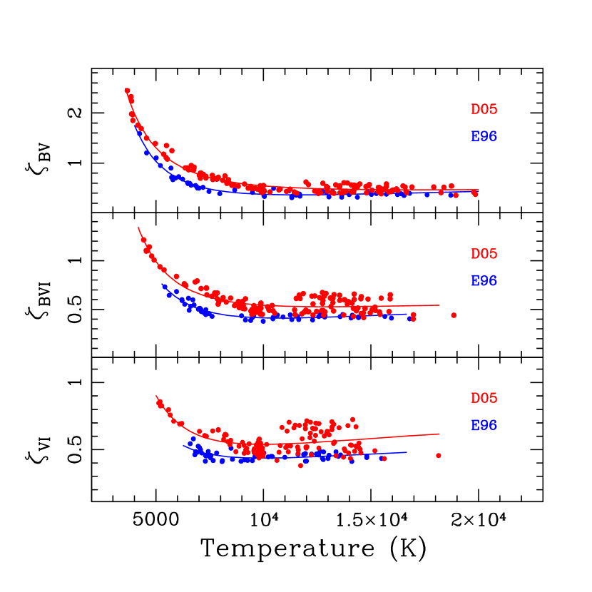
Figure 4: Dilution factors $\zeta$ as a function of the color temperature, computed at $z=0$ from the E96 (blue dots) and D05 (red dots) atmosphere models for three different filter subsets ($\{BV\},\{BVI\},\{VI\}$). The blue (red) line correspond to the polinomial fit performed to the E96 (D05) dilution factors.  

where $S(\lambda)$ is the filter transmision function and $ZP$ the zero point of the photometric system (Hamuy et al., 2001). The constant $h$ and $c$ are the Planck constant and the speed of light, respectively. Clearly the dilution factors depend on the specific redshift of the SN and on the filter subset used to obtained the color temperature of the models. Figure 4 shows the resulting dilution factors versus temperature at $z=0$. We performed polynomial fits to $\zeta(T_{s})$ of the form

$$\zeta(T_{s})=\sum_{j=0}^{2}b_{s,j}\left(\frac{10^{4}K}{T_{s}}\right)^{j}$$ (7)

Table 3 lists the $b_{s,j}$ coefficients at $z=0$ for three filter subsets and both atmosphere models, E96 and D05. The corresponding polinomial fits are shown as solid lines in Figure 4.
The D05 dilution factors are quite insensitive to the color temperature above $\sim$ $9000$ $K$, and lie around 0.5, while at lower temperature they increase sharply with decreasing temperature, reaching a value over unity below $\sim$ $5000$ $K$. The E96 dilution factors present the same pattern, but they are systematically lower than the D05 dilution factors by $\sim$ $15\%$. The origin of these differences is unclear. Dessart & Hillier (2005a) discuss that the discrepancy might be related to the different approach used to handle the relativistic terms. Also, D05 solved the non-Local Thermodynamic Equilibrium (non-LTE) for all the species, and employed a very complex atom model. E96, on the other hand, solved the non-LTE problem for a few species and for the rest of the metals the excitation and ionization were assumed to be given by the Saha-Boltzmann equation, and the opacity was taken as pure scattering. Another important difference between the E96 and D05 dilution factors is the dependence on the parameters involved in the atmosphere modelling. While the E96 dilution factors show little sensivity to a broad range of phyical parameters other than temperature, the D05 models show a larger dispersion at a given color temperature. On average, the E96 models lead to a dispersion of $\sigma\sim 0.03$ in $\zeta$, while the D05 models yield to $\sigma\sim 0.07$.

3.3 Angular radii

An apparent angular radius ($\theta\zeta_{s}$) and a color temperature ($T_{s}$) of the SN can be obtained by fitting a Planck function $B_{{\lambda^{{}^{\prime}}}}(T_{s})$ to the observed broad band magnitudes (see eq. 1). Here S is the filter subset combination, i.e., $S=\{BV\},\{BVI\},\{VI\}$. Since we have two unknowns ($\theta\zeta_{s}$,$T_{s}$), the subsets must contain at least two filters. In order to derive these parameters, we used a least-squares technique at each spectroscopic observation epoch (see $\S$ 3.6), by minimizing the quantity

$$\chi^{2}=\sum_{s}\frac{[m_{\overline{\lambda}}+5log(\theta\zeta_{s,z})-b_{\overline{\lambda}}(T_{s},z)]^{2}}{\sigma_{m}^{2}}$$ (8)

Here $m_{\overline{\lambda}}$ is the apparent magnitude in the filter with central wavelength $\overline{\lambda}$, i.e., $m_{\overline{\lambda}}\in\{B,V,I\}$, $\sigma_{m}$ is the photometric error in the magnitude $m_{\overline{\lambda}}$ and $b_{\overline{\lambda}}$ is defined in eq. 6. Because $\zeta_{s}$ is mainly a function of the color temperature (Figure 4), it is possible to use $T_{s}$ to solve for $\zeta_{s}$ and determine the true angular radius $\theta$, from $\theta\zeta_{s}$.

3.4 Physical radii

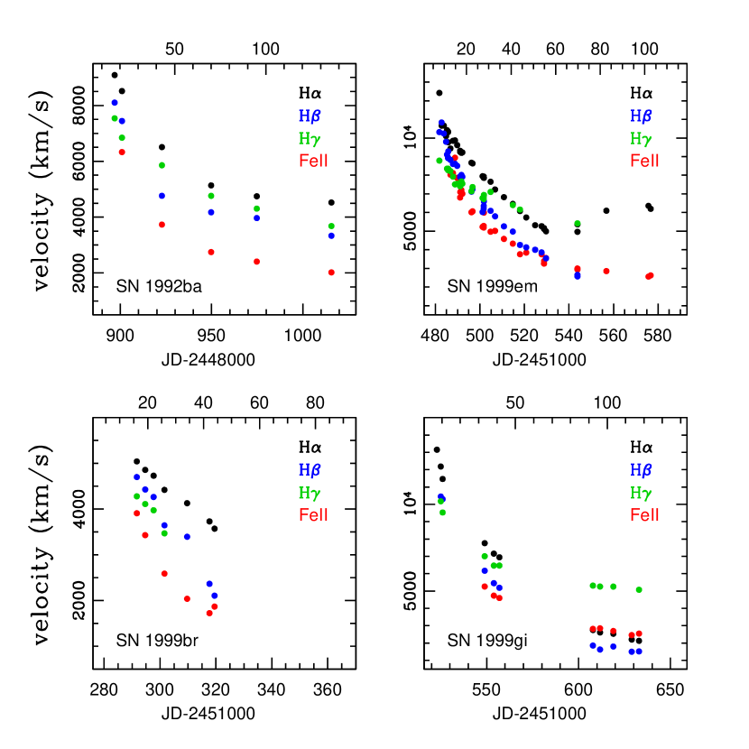
Figure 5: Line velocity evolution determined from the P Cygni absorption minima of four different features during $\sim$ 100 days after discovery. In the top of each panel is shown the date since the EPM explosion time derived using the D05 models (see Table 7).  

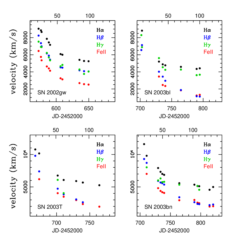
Figure 6: Line velocity evolution determined from the P Cygni absorption minima of four different features during $\sim$ 100 days after discovery. In the top of each panel is shown the date since the EPM explosion time derived using the D05 models (see Table 7).  

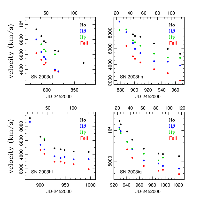
Figure 7: Line velocity evolution determined from the P Cygni absorption minima of four different features during $\sim$ 100 days after discovery. In the top of each panel is shown the date since the EPM explosion time derived using the D05 models (see Table 7).  

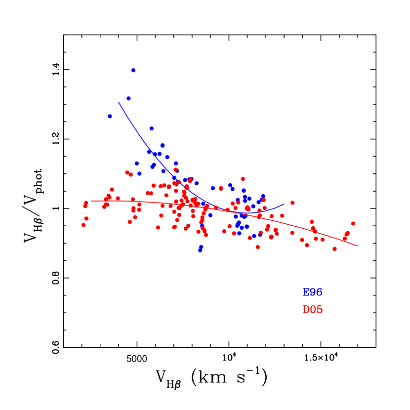
Figure 8: Ratio between the H$\beta$ and the photospheric velocity versus the H$\beta$ velocity of the individual SN models. The blue dots correspond to E96 models and the red dots to D05 models. The blue (red) line corresponds to the polinomial fit performed to the E96 (D05) photospheric velocity conversion.  

Once $\theta$ is determined, the next step is to measure the photospheric velocity (see eq. 3). The photospheric velocity of the SN at a given epoch can be obtained from the absorption lines in the spectra. Table 4 lists the spectroscopic velocities measured from the minima of H$\alpha$, H$\beta$, H$\gamma$ and Fe ii $\lambda 5169$ lines, for all 12 SNe. Figures 5-7 show the temporal evolution of the spectral line velocities.
To date the photospheric velocities have been estimated using weak spectral absorption features such as Fe ii lines $\lambda 5169$, $\lambda 5018$, $\lambda 4924$ and Sc ii $\lambda 4670$ (Schmidt et al., 1992; Leonard et al., 2002). The physical assumption is that these lines are optically thin and are formed near the photosphere of the SN. However, there are two problems with this approach: 1) at early times the spectra are dominated by Balmer lines and the weak lines are absent and 2) the synthetic spectra show that even the weak lines do not necessarily yield true photospheric velocities (Dessart & Hillier, 2006). One way to circumvent these problems is to use the Balmer lines which are present in the spectra over most of the evolution of the SN. Although the Balmer lines are much more optically thick than the Fe ii lines, Dessart & Hillier (2006) argued that, contrary to what is usually believed, optically thick lines do not necessarilly overestimate the photospheric velocity, and the offset from the photospheric velocity can be measured from the synthetic spectra. In this work we decided to use the minimum of the H$\beta$ absorption line to derive the photospheric velocity because this line is present during all the plateau phase, it can be easily identified, and it does not present any blend, at least in the first $\sim$ 50 days after explosion.
To convert from observed H$\beta$ spectroscopic velocities to true photospheric velocities we used the synthetic spectra from E96 and D05. Figure 8 shows (in red) the ratio of H$\beta$ velocity and the photospheric velocity, as a function of H$\beta$ velocity for all the D05 models. Note that the D05 models predict that the H$\beta$ line forms quite close to the photosphere at all epochs (for all values of $v_{H\beta}$). Also plotted in Figure 8 (in blue) are the E96 models which confirms that the H$\beta$ forms close to the photosphere at early epochs, when the $v_{H\beta}$ is high. However, at later epochs (lower $v_{H\beta}$) E96 predict that H$\beta$ forms in outer layers (higher velocities) than D05. Also it is important to note that the E96 models cover a shorter range in velocity ($\sim$ $4500-12000$ $km$ $s^{-1}$) than the D05 models ($\sim$ $2000-17000$ $km$ $s^{-1}$), which restricts the EPM analysis using the E96 models.
To derive the ratio between the H$\beta$ and the photospheric velocity we used a polinomial fit (as plotted in Figure 8) of the form

$$\frac{v_{H\beta}}{v_{phot}}=\sum_{j=0}^{2}a_{j}(v_{H\beta})^{j}$$ (9)

The $a_{j}$ coefficients are listed in Table 5. The E96 models lead to a dispersion of $\sigma=0.06$ and the D05 models to $\sigma=0.04$. The photospheric velocity $v_{i}$ can be obtained from a measurement of $v_{H\beta}$

$$v_{i}=\frac{v_{H\beta}}{\displaystyle{\sum_{j=0}^{2}a_{j}(v_{H\beta})^{j}}}$$ (10)

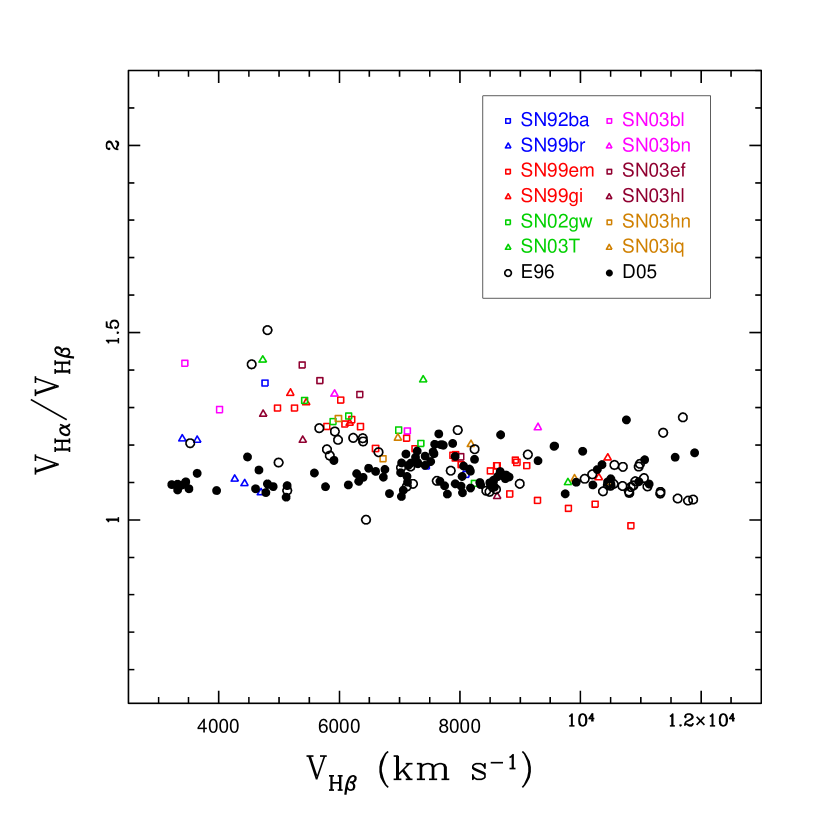
Figure 9: Ratio between the H$\alpha$ and H$\beta$ velocity as a function of the H$\beta$ velocity. The triangles and the squares represent velocities measured from the spectra of our SN sample. The open and filled black circles correspond to the velocity ratio measured from the synthetic spectra of E96 and D05 respectively .  

In order to examine which of the adopted photospheric velocity conversion was closer to reality, we compared the ratio between the H$\alpha$ and H$\beta$ velocities measured from the observed spectra of our sample of SNe and from the synthetic spectra of the E96 and D05 models. Figure 9 shows the $H\alpha/H\beta$ velocity ratio as a function of the H$\beta$ velocity. It can be seen that, while there is good agreement between theory and observations at high H$\beta$ velocities ($\sim$ 6500 - 10500 $km$ $s^{-1}$), the D05 models underestimate the H$\alpha$ velocities (or overestimate the H$\beta$ velocities) at lower expansion velocities, while the $H\alpha/H\beta$ velocity ratio predicted by the E96 models is in good agreement with the observations at all H$\beta$ velocities. This suggests that E96 predict more realistic line profiles in the SN ejecta than D05 and therefore should provide a better photospheric velocity conversion.

3.5 Extinction

To estimate the amount of Galactic foreground extinction we used the IR dust maps of Schlegel et al. (1998). Table 6 summarizes the foreground extinction adopted. In this work we adopted two different methods for host galaxy reddenings of our SN sample, a spectroscopic method (DES hereafter), and a method based on the color evolution of the SNe (OLI hereafter). The former was developed by Dessart (2008) and consists in fitting different model spectra to the early time spectra of a SN. The two fitting parameters are the amount of reddening and the photospheric temperature. The color-based technique was developed by Olivares et al. (2008) and is based on the assumption that the color at the end of the plateau phase is the same for all SNe IIP. In both cases they adopted the Cardelli et al. (1989) extinction law (with $R_{V}=3.1$). Table 6 lists the host galaxy visual extinction values $A_{V}$ obtained from both methods. Also, in Figure 10 are plotted the OLI versus DES visual extinctions. As can be seen, there are no systematic differences between both models. However, there are individual differences, specially in five SNe, in which cases their names are explicitly marked in the plot.

3.6 Implementation of EPM

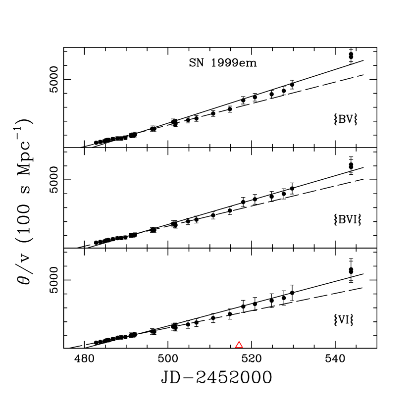
Figure 11: $\theta/v$ as a function of time for SN 1999em using the $\{BV\}$, $\{BVI\}$ and $\{VI\}$ filter subsets and the D05 models. The solid (dashed) lines correspond to unweighted least-squares fits to the derived EPM quantities using $\sim$ 70 (40) days after explosion. The red triangle in the bottom panel shows the day $\sim$ 40 after explosion.  

The EPM method is only valid in the optically thick phase of a H-rich expanding atmosphere. Observationally this period corresponds to the plateau phase of Type II SNe and thus justifies our first selection criterion in $\S$ 2.3.
The EPM requires at least two simultaneaus photometric and spectroscopic observations (see eq. 3), but we recommend the use of at least three points in order to obtain an internal check. The photometry is used to determine the angular size of the SN and the spectroscopy is used to measure the expansion velocities of the SN. The requirement of simultaneous photometric and spectroscopic observations is not always accomplished because most of the time the photometry and the spectroscopy of a SN are taken at different epochs. To overcome this problem, it is necessary to interpolate the photometry or the velocities measured from the spectroscopy. In this work we decided to interpolate the photometry for two reasons: 1) the number of photometric observations in our sample of SNe is far greater than the number of spectroscopic observations and 2) the optical apparent magnitude of the Type II-P SNe is nearly constant during the plateau phase, which makes the interpolation more reliable than the velocity interpolation, which has a steeper dependence with time. To interpolate a magnitude at the epoch of a given spectroscopic observation we use a quadratic polynomial fit, using four neighboring points, i.e., four photometric observations around the spectroscopic date.
In this study, we restricted the EPM analysis to the first $\sim 45-50$ days after explosion because there is a clear departure from linearity in the $\theta/v$ versus $t$ plots after this date. In Figure 11 are plotted the EPM solutions for SN 1999em (because it has extensive photometric and spectroscopic observations during the plateau phase) using the $\{BV\},\{BVI\}$ and $\{VI\}$ filter subsets and the D05 models. The solid line corresponds to the least-squares fit to the derived EPM quantities using the first $\sim$ 70 days after explosion, while the dashed line correspond to the least-squares fit using only the first $\sim$ 40 days after explosion. As can be noted, after $\sim$ 40 days from explosion (marked with a red triangle) there is departure from the linear $\theta/v$ versus $t$ relation in all three cases. This justifies our second and third selection criteria in $\S$ 2.3. This restriction severely lowers the number of SNe of our sample to which we can apply the EPM. Out of the initial 51 SNe of the Hamuy et al. (2008) sample, only 11 objects fulfill the requirement of having a plateau behavior and having early time photometry and spectroscopy for the EPM analysis.

3.6.1 EPM analysis to individual SNe

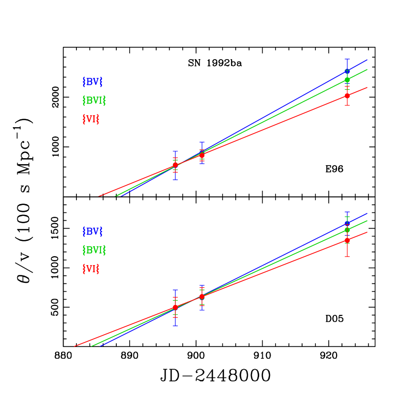
Figure 12: $\theta/v$ as a function of time for SN 1992ba using the $\{BV\}$, $\{BVI\}$ and $\{VI\}$ filter subsets. The ridge lines correspond to unweighted least-squares fits to the derived EPM quantities. The upper and lower panel shows the results using E96 and D05 dilution factors respectively. In all cases we employ the DES reddening.  

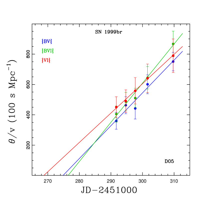
Figure 13: $\theta/v$ as a function of time for SN 1999br using the $\{BV\}$, $\{BVI\}$ and $\{VI\}$ filter subsets and the D05 models. The ridge lines correspond to unweighted least-squares fits to the derived EPM quantities. In all cases we employ the DES reddening.  

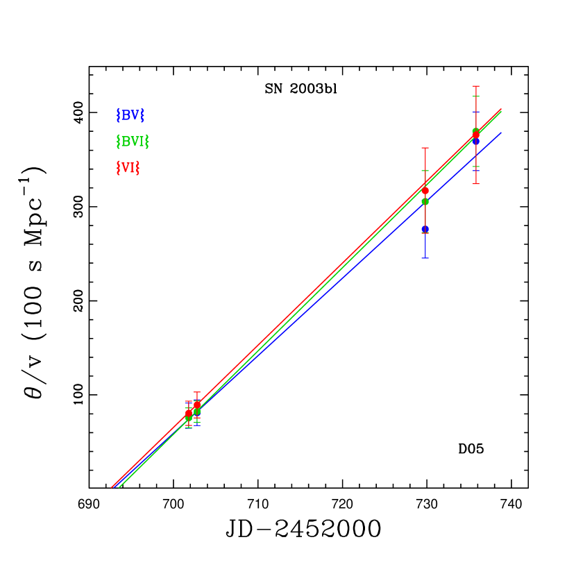
Figure 18: $\theta/v$ as a function of time for SN 2003bl using the $\{BV\}$, $\{BVI\}$ and $\{VI\}$ filter subsets and the D05 models. The ridge lines correspond to unweighted least-squares fits to the derived EPM quantities. In all cases we employ the DES reddening.  

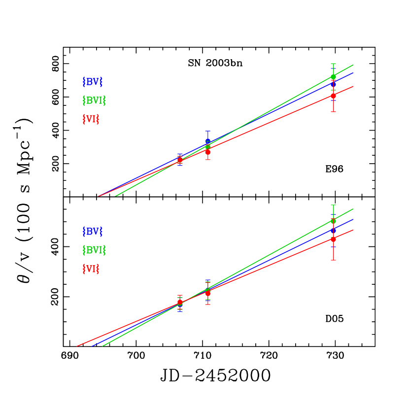
Figure 19: $\theta/v$ as a function of time for SN 2003bn using the $\{BV\}$, $\{BVI\}$ and $\{VI\}$ filter subsets. The ridge lines correspond to unweighted least-squares fits to the derived EPM quantities. The upper and lower panel shows the results using E96 and D05 dilution factors respectively. In all cases we employ the DES reddening.  

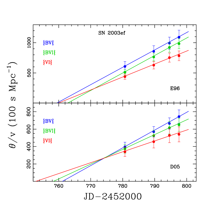
Figure 20: $\theta/v$ as a function of time for SN 2003ef using the $\{BV\}$, $\{BVI\}$ and $\{VI\}$ filter subsets. The ridge lines correspond to unweighted least-squares fits to the derived EPM quantities. The upper and lower panel shows the results using E96 and D05 dilution factors respectively. In all cases we employ the DES reddening.  

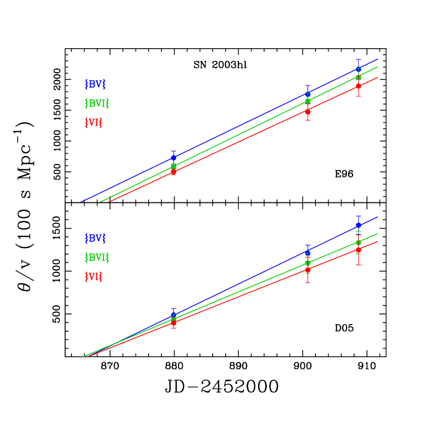
Figure 21: $\theta/v$ as a function of time for SN 2003hl using the $\{BV\}$, $\{BVI\}$ and $\{VI\}$ filter subsets. The ridge lines correspond to unweighted least-squares fits to the derived EPM quantities. The upper and lower panel shows the results using E96 and D05 dilution factors respectively. In all cases we employ the DES reddening.  

In this section we present the EPM analysis for 12 SNe IIP (11 from our database and one from the literature) with early spectroscopic and photometric observations. We carried out the analysis using three different filter subsets ({BV}, {BVI}, {VI}), two sets of host galaxy extinctions (OLI, DES) and two atmosphere models (E96, D05), which yields a total of 12 solutions for each SN. The tables that summarize the EPM quantities are available in electronic format for all 144 cases. In the remainder of this section we restrict the presentation to the 6 solutions that use the DES extinction because they give the lowest dispersion in the Hubble diagrams. Figures 12-23 show these 6 solutions for each of the 12 SNe. In the following, we provide the EPM distance $D$ and the explosion date $t_{0}$ and their uncertainties, using DES and the {VI} filter subset, and we compare the time of explosion to the range restricted by pre-SN images of the host galaxies. These results are also summarized in Table 7. In order to obtain a more realistic estimation of the error in the distance and the explosion date, we computed 100 Monte Carlo simulations for each SN, in which we varied all the parameters involved in the EPM (see Table 8), and we averaged the 100 distances and explosion dates to derive the EPM $D$ and $t_{0}$. This produces small differences between the results computed from the initial single EPM solution and that obtained from the 100 Monte Carlo simulations, but the latter provides a much more realistic estimate of the uncertainties. Finally, in Tables 9-20 we reproduce the results (computing the 100 Monte Carlo simulations) for each SN using the specific $\{VI\}$, DES and D05 combination, which leads to the lowest dispersion in the Hubble diagrams among all 12 possible combinations.

SN 1992ba

Figure 12 shows $\theta/v$ versus time for SN 1992ba using the $\{BV\},\{BVI\}$ and $\{VI\}$ filter subsets and the E96 and D05. Table 9 summarizes the EPM quantities derived from the $\{VI\}$ filter subset and the D05 models. We used 3 epochs (JD 2448896.9 - 2448922.8) to compute the distance to this SN. In order to use the velocities measured on JD 2448896.9 and 24448900.9 we had to extrapolate the $I$ band photometry until JD 2448896.9.
SN 1992ba was discovered by Evans (1992) on JD 2448896.3. McNaught (1992) reported that the SN was not present on a plate taken on JD 2448883.2 with limiting magnitude 19. The EPM solution yields $t_{0}$ = 2448883.9 $\pm$ 3.0 using the E96 models and $t_{0}$ = 2448879.8 $\pm$ 5.6 with D05. These results agree (within one $\sigma$) with the explosion date constrained by the pre and post explosion observations. The distances derived to SN 1992ba are $D$ = 16.4 $\pm$ 2.5 Mpc and $D$ = 27.2 $\pm$ 6.5 Mpc using the E96 and the D05 dilution factors, respectively.

SN 1999br

Figure 13 shows $\theta/v$ versus time for SN 1999br using the $\{BV\},\{BVI\}$ and $\{VI\}$ filter subsets and the D05 models. Table 10 summarizes the EPM quantities from the $\{VI\}$ filter subset and the D05 models. We used 5 epochs (JD 2451291.7 - 2451309.7) to compute the distance to this SN. The EPM solution shows some departure from linearity using the {BV} and {BVI} filter subsets. SN 1999br presents very low expantion velocities, therefore we were unable to obtain its distance using the E96 models. This is because the photospheric velocity conversion factor $V_{H\beta}/V_{phot}$ is not defined at low expansion velocities (see $\S$ 3.4 and Figure 8). The EPM solution yields $t_{0}$ = 2451275.6 $\pm$ 7.7 using the D05 models. This result compare very well with the observations, because SN 1999br was discovered by the Lick Observatory Supernova Search (LOSS) on JD 2451280.9 (King, 1999). An image taken on JD 2451264.9 showed nothing at the SN position at a limiting magnitudes of 18.5 (Li, 1999a). The EPM distance to SN 1999br is $D$ = 39.5 $\pm$ 13.5 Mpc using the D05 dilution factors.

SN 1999em

SN 1999em is the best ever observed SN IIP. Many photometric and spectroscopic observations were made by different observers during the plateau phase. Figure 14 shows $\theta/v$ versus time for the SN 1999em using the $\{BV\},\{BVI\}$ and $\{VI\}$ filter subsets and the E96 and D05 models. Table 11 summarizes the EPM quantities derived from the $\{VI\}$ filter subset. We used 25 epochs (JD 2451482.8 - 2451514.8) to derive the distance to SN 1999em. Four spectra were taken from Hamuy et al. (2001) and the other 21 from Leonard et al. (2002). In some cases there were two spectra taken at the same epoch from both sources. In those cases we used them individuallly in the EPM solution instead of averaging the measured velocities from each spectrum. We removed the first spectrum (JD 2451481.8) from the EPM solution because it shows a clear departure from the linear $\theta/v$ versus $t$ relation. The EPM solutions using E96 and D05 are quite linear and show great detail in the evolution of $\theta/v$ due to the high quality spectroscopic and photometric coverage. However, the E96 solution shows a small departure from linearity in the last two spectroscopic epochs. This effect is probably due to the high rise in the $V_{H\beta}/V_{phot}$ ratio at low velocities in the E96 models.
SN 1999em was discovered on JD 2451480.9 by the LOSS program (Li, 1999b). An image taken at the position of the SN on JD 2451472.0 showed nothing at a limiting magnitude of 19.0. The EPM yields $t_{0}$ = 2451476.3 $\pm$ 1.1 and $t_{0}$ = 2451474.0 $\pm$ 2.0 using the E96 and D05 models. These explosions dates are between the pre-discovery and the discovery date. The distances derived to SN 1999em are $D$ = 9.3 $\pm$ 0.5 Mpc from E96 and $D$ = 13.9 $\pm$ 1.4 Mpc from D05.

SN 1999gi

Figure 15 shows $\theta/v$ versus time for SN 1999gi using the $\{BV\},\{BVI\}$ and $\{VI\}$ filter subsets and the E96 and D05 models. Table 12 summarizes the EPM quantities derived from the $\{VI\}$ filter subset. We used 5 epochs (JD 2451525.0 - 2451556.9) to apply the EPM method. All the spectra and the photometry were taken from Leonard et al. (2002b). The first spcetrum (JD 2451522.9) was remove from the EPM solutions because it yields an H$\beta$ velocity of $\sim 26.000$ $km$ $s^{-1}$, well above the range of the photospheric velocity conversion (see $\S$ 3.4 and Figure 8). The explosion dates of SN 1999gi obtained using the EPM are $t_{0}$ = 2451517.0 $\pm$ 1.2 using E96 models and $t_{0}$ = 2451515.6 $\pm$ 2.4 with D05. These results agreed with the observations because a pre-discovery image taken on JD 2451515.7 (Trondal et al., 1999) showed nothing at the SN position (limiting unfiltered magnitude of 18.5). SN 1999gi was discovered on JD 2451522.3 (Nakano, Sumoto, Kushida, 2002) on unfiltered CCD frames, so the explosion date can be constrained in a range of only 6.6 days. We derive a distance of $D$ = 11.7 $\pm$ 0.8 and $D$ = 17.4 $\pm$ 2.3 Mpc using the E96 and D05 models, respectively.

SN 2002gw

Figure 16 shows $\theta/v$ versus time for SN 2002gw using the $\{BV\},\{BVI\}$ and $\{VI\}$ filter subsets and the E96 and D05 models. Table 13 summarizes the EPM quantities from the $\{VI\}$ filter subset. The EPM solutions were obtained using 6 epochs (JD 2452573.1 - 2452590.7). The EPM yields explosion times of $t_{0}$ = 2452557.9 $\pm$ 2.7 and $t_{0}$ = 2452551.7 $\pm$ 7.6 (using E96 and D05 dilution factors, respectively). SN 2002gw was discovered on JD 2452560.8 (Monard, 2002). An image taken on JD 2452529.6 shows nothing at the SN position at a limiting magnitude of 18.5. Also, an unfiltered CCD image taken on JD 2452559.1 shows the SN at magnitude 18.3 (Itagaki & Nakano, 2002). The EPM explosion dates are in agreement with the SN explosion date constrained by the observations. The EPM distances are $D$ = 37.4 $\pm$ 4.9 Mpc and $D$ = 63.9 $\pm$ 17.0 Mpc using E96 and D05, respectively.

SN 2003T

Figure 17 shows $\theta/v$ versus time for SN 2003T using the $\{BV\},\{BVI\}$ and $\{VI\}$ filter subsets and the E96 and D05 models. Table 14 summarizes the EPM quantities from the $\{VI\}$ filter subset. The EPM explosion dates are $t_{0}$ = 2452654.2 $\pm$ using E96 models and $t_{0}$ = 2452648.9 $\pm$ 3.4 with D05. In both cases the third epoch used to derive the distance is beyond $\sim$ 45 ays after the EPM $t_{0}$, but it proves neccesary to include it to compute the EPM analysis. This SN was discovered by LOTOSS on JD 2452664.9 (Schwartz & Li, 2003). An image taken on JD 2452644.9 shows nothing at a limiting magnitude of 19.0, in good agreement with the EPM analysis. The EPM distances are $D$ = 87.8 $\pm$ 13.5 Mpc using E96 and $D$ = 147.3 $\pm$ 35.7 Mpc with D05.

SN 2003bl

Figure 18 shows $\theta/v$ versus time for SN 2003bl using the $\{BV\},\{BVI\}$ and $\{VI\}$ filter subsets and D05 models. Table 15 summarizes the EPM quantities derived for SN 2003bl from the $\{VI\}$ filter subset. The EPM solutions were obtained using 4 epochs (JD 2452701.8 -2452735.8). As with the SN 1999br, we were unable to apply the EPM using E96 because we only had two spectra with velocities higher than $4500$ $km$ $s^{-1}$, and so the photospheric velocity correction could not be applied (see $\S$ 3.4 and Figure 8). SN 2003bl was discovered by LOTOSS on JD 2452701.0 (Swift, Weisz & Li, 2003). A pre-discovery image taken on JD 2452438.8 shows nothing at the SN position at a limiting magnitud of 19.0. The EPM yields $t_{0}$ = 2452692.6 $\pm$ 2.8, consistent with the SN discovery date . The EPM distance is $D$ = 92.4 $\pm$ 14.2 Mpc.

SN 2003bn

Figure 19 shows $\theta/v$ versus time for SN 2003bn using the $\{BV\},\{BVI\}$ and $\{VI\}$ filter subsets and the E96 and D05 models. Table 16 summarizes the EPM quantities from the $\{VI\}$ filter subset. We computed the EPM analisys using 3 epochs (JD 2452706.6 - 2452729.7). The EPM yields explosions dates of $t_{0}$ = 2452693.4 $\pm$ 2.7 and $t_{0}$ = 2452687.0 $\pm$ 9.0 from E96 and D05, respectively. SN 2003bn was discovered on JD 2452698.0 (Wood-Vasey, Aldering & Nugent, 2003). Two pre-discovery NEAT images shows nothing at the SN position on JD 2452691.5 (limiting magnitude of 21.0) and the SN at a magnitude of 20.2 on JD 2452692.8, which restricted the explosion date in a range of only 1.3 days. This value for $t_{0}$ is in agreement within one $\sigma$ with the EPM $t_{0}$ derived using E96 and D05. The EPM distances from E96 and D05 are $D$ = 50.2 $\pm$ 7.0 Mpc and $D$ = 87.2 $\pm$ 28.0 Mpc, respectively.

SN 2003ef

Figure 20 shows $\theta/v$ versus time for SN 2003ef using the $\{BV\},\{BVI\}$ and $\{VI\}$ filter subsets and the E96 and D05 models. Table 17 summarizes the EPM quantities from the $\{VI\}$ filter subset. We computed the EPM analysis using 4 epochs (JD 2452780.7 -2452797.6). The explosion date derived are $t_{0}$ = 2452759.8 $\pm$ 4.7 and $t_{0}$ = 2452748.4 $\pm$ 15.6 with E96 and D05, respectively. SN 2003ef was discovery by the LOTOSS on JD 2452770.8 (mag. about 16.3) (Weisz & Li, 2003), consistent with the EPM $t_{0}$. A KAIT image taken on JD 2452720.8 showed nothing at the SN position at a limiting magnitude of 18.5. The EPM distances are $D$ = 38.7 $\pm$ 6.53 Mpc with E96 and $D$ = 74.4 $\pm$ 30.3 Mpc with D05.

SN 2003hl

Figure 21 shows $\theta/v$ versus time for SN 2003hl using the $\{BV\},\{BVI\}$ and $\{VI\}$ filter subsets and the E96 and D05 models. Table 18 summarizes the EPM quantities derived from the $\{VI\}$ filter subset. The EPM solutions were obtained using 3 epochs (JD 2452879.9 -2452908.7). We estimated the explosion dates on $t_{0}$ = 2452872.3 $\pm$ 1.7 and $t_{0}$ = 2452865.4 $\pm$ 5.9 using E96 and D05, respectively. SN 2003hl was discovered on JD 2452872.0 during the LOTOSS program at a magnitude of 16.5 (Moore, Li, & Boles, 2003). A pre-discovery KAIT image taken on JD 2452863.0 shows nothing at the SN position at a limiting magnitude of 19.0. This image restricts the explosion date in a range of 9 days. The EPM explosion dates are in agreement with the observations (within one $\sigma$). We derived EPM distances of $D$ = 17.7 $\pm$ 2.1 Mpc with E96 and $D$ = 30.3 $\pm$ 6.3 Mpc with D05.

SN 2003hn

Figure 22 shows $\theta/v$ versus time for SN 2003hn using the $\{BV\},\{BVI\}$ and $\{VI\}$ filter subsets and the E96 and D05 models. Table 19 summarizes the EPM quantities from the $\{VI\}$ filter subset. The EPM solutions were obtained using 4 epochs (JD 2452878.2 - 2452900.9). The EPM explosion dates derived are $t_{0}$ = 2452859.5 $\pm$ 3.8 and $t_{0}$ = 2452853.8 $\pm$ 9.3 using the E96 and D05 dilution factors, respectively. This SN was discovered on JD 2452877.2 at mag. 14.1 by Evans (2003). Evans also reported that the SN was not visible at mag. 15.5 on JD 2452856.5. This date agrees with the explosion date derived from E96 and is less than one $\sigma$ lower than that derived from D05. The EPM solutions leads to $D$ = 16.9 $\pm$ 2.2 Mpc and $D$ = 26.3 $\pm$ 7.1 Mpc using E96 and D05, respectively.

SN 2003iq

Figure 23 shows $\theta/v$ versus time for SN 2003iq using the $\{BV\},\{BVI\}$ and $\{VI\}$ filter subsets and the E96 and D05 models. Table 20 summarizes the EPM quantities from the $\{VI\}$ filter subset. The EPM solutions were obtained using 4 epochs (JD 2452928.7 - 2452948.7). This SN was discovered by LLapasset (2003) on JD 2452921.5, while monitoring SN 2003hl in the same host galaxy. A pre-discovery image taken on 2452918.5 shows nothing at the SN position. These reports constrain the explosion date to a range of only three days. The EPM yields $t_{0}$ = 2452909.6 $\pm$ 4.3 using E96 and $t_{0}$ = 2452905.6 $\pm$ 9.5 using D05. In both cases the explosion date is far earlier than expected because the SN was not present on JD 2452918.5. This implies that the EPM solutions to this SN are not satisfactory. We derived EPM distances of $D$ = 36.0 $\pm$ 5.6 Mpc with $E96$ and D = 53.3 $\pm$ 17.1 Mpc with D05.

4 Discussion

4.1 External comparison

• Previous EPM distances.

  The EPM method has been already applied to SN 1999em by other authors. Hamuy et al. (2001) employed the E96 dilution factors and eight different filter subsets to perform the EPM analysis to this SN. They used a cross-correlation technique to estimate the photospheric velocity and adopted a host galaxy extinction of $A_{V}=0.18$. They derived a distance of 6.9 $\pm$ 0.1, 7.4 $\pm$ 0.1 and 7.3 $\pm$ 0.1 Mpc from the $\{BV\}$, $\{BVI\}$ and $\{VI\}$ filter subsets, respectively. These values are in agreement with our estimates of 6.9 $\pm$ 0.6, 7.5 $\pm$ 0.6 and 9.3 $\pm$ 0.5 Mpc (from the $\{BV\}$, $\{BVI\}$ and $\{VI\}$ filter subsets, respectively), except in the $\{VI\}$ case. Also Leonard et al. (2002) employed the E96 models to derive the distance to SN 1999em. They used four weak unblended spectral features (Fe ii 4629, 5276, 5318 and Sc ii $\lambda$4670) as the photospheric velocity indicators. They adopted a host galaxy reddening of $A_{V}=0.31$, the same value predicted by DES. They derived a distance of 7.7 $\pm$ 0.2, 8.3 $\pm$ 0.2 and 8.8 $\pm$ 0.3 Mpc from the $\{BV\}$, $\{BVI\}$ and $\{VI\}$ filter subsets, respectively. These results are in agreement with our E96 distances. Finally, Dessart & Hillier (2006) applied the EPM method to SN 1999em using E96 and D05. They adopted the SN 1999em DES reddening value of $A_{V}=0.31$. Using the E96 models, they derived a distance of 8.6 $\pm$ 0.8, 9.7 $\pm$ 1.0 and 11.7 $\pm$ 1.5 Mpc from the $\{BV\}$, $\{BVI\}$ and $\{VI\}$ filter subsets, respectively, which are somewhat greater than our distances. Using the D05 models they derived a distance of 13.5 $\pm$ 1.5, 12.5 $\pm$ 1.6 and 14.6 $\pm$ 1.9 Mpc from the $\{BV\}$, $\{BVI\}$ and $\{VI\}$ filter subsets, respectively, which are significantly larger than our values of 11.2 $\pm$ 0.2, 12.0 $\pm$ 0.2 and 14.0 $\pm$ 0.2 Mpc, respectively. This is probably due to a different implementation of the EPM.

• SEAM distance The Spectral-fitting Expanding Atmosphere Method (SEAM) is a similar technique to the EPM, but it avoids the use of dilution factors and includes the synthetic spectral fitting to the observed spectra of the SN. Baron et al. (2004) applied this method to SN 1999em. They derived a distance of $D=12.5\pm 2.3$ Mpc, in good agreement with our distances derived using the D05 models (11.2 $\pm$ 0.2, 12.0 $\pm$ 0.2 and 14.0 $\pm$ 0.2 Mpc from the $\{BV\}$, $\{BVI\}$ and $\{VI\}$ filter subsets, respectively), but significantly greater than the EPM distances derived using E96 (6.9 $\pm$ 0.6, 7.5 $\pm$ 0.6 and 9.3 $\pm$ 0.5 Mpc from the $\{BV\}$, $\{BVI\}$ and $\{VI\}$ filter subsets, respectively).

• Cepheid distance

  Leonard et al. (2003) identified 41 Cepheid variable stars in NGC 1637, the host galaxy of SN 1999em. They derived a Cepheid distance to NGC 1637 of $D=11.7\pm 1.0$ Mpc. As with the SEAM results, the Cepheid distance is consistent with our EPM distances derived using the D05 models (11.2 $\pm$ 0.2, 12.0 $\pm$ 0.2 and 14.0 $\pm$ 0.2 Mpc from the $\{BV\}$, $\{BVI\}$ and $\{VI\}$ filter subsets, respectively). In all cases, the E96 models lead to significantly lower distances (6.9 $\pm$ 0.6, 7.5 $\pm$ 0.6 and 9.3 $\pm$ 0.5 Mpc from the $\{BV\}$, $\{BVI\}$ and $\{VI\}$ filter subsets, respectively).

4.2 Error analysis

4.2.1 Effects of reddening

While the Schlegel et al. (1998) IR maps provide a precise estimate of the amount of Galactic foreground extinction, the determination of host galaxy extinction is a more challenging task. This is a potential problem because the distances derived using EPM depend on the adopted host galaxy extinction. In order to investigate the sensitivity of the distances to dust extinction, we performed the EPM analysis to all the SNe in our sample using the $\{VI\}$ filter subset by varying the amount of host galaxy visual extinction $A_{V}$ in steps of $\Delta A_{V}=0.1$ mag. Figure 24 shows the normalized EPM distances as a function of host galaxy visual extinction $A_{V}$ relative to the DES value ($\Delta A_{V}=0$). As can be seen, the EPM is quite insensitive to the amount of host galaxy extinction adopted. On average, the distances change by less than $\sim 10\%$ from $\Delta A_{V}$ = 0.0 to $\Delta A_{V}$ = 0.5 and by less than $\sim 20\%$ going from $\Delta A_{V}$ = 0.0 to $\Delta A_{V}=-0.5$. Therefore, even a systematic error of 0.5 in $A_{V}$, produces a small error in the EPM distance.

4.2.2 Other sources of error

Table 8 lists all the error sources in EPM and their typical values. In order to investigate which source contributes the most to the uncertainty in the EPM distance, we performed the EPM analysis to SN 1999gi (whose photometry and spectroscopy coverage is representative of our sample) and we changed the error of a single source (listed in Table 8) leaving all others unchanged. We found two main sources of errors. In the E96 case, the errors in the photospheric velocity conversion and the dilution factors have the largest effect in the distance uncertainty, each one contributing $\sim 30\%$ of the total error, while in the D05 case the error in the dilution factors produces $\sim 70\%$ of the uncertainty in the distance, far greater than that due to the error in the photospheric velocity conversion ($\sim 10\%$ of the total error). All of the other errors have a secondary effect in the total error.

4.3 Hubble Diagrams

Since the discovery of the expansion of the Universe (Hubble, 1929), the determination of the expansion rate, the Hubble constant ($H_{0}$), has become one of the most important challenges in astronomy and cosmology. Using the velocity-distance relation (Hubble diagram) calibrated using the Cepheid period-luminosity relation, (Hubble & Humason, 1931) obtained $H_{0}$ $\sim$ 500 $km$ $s^{-1}$ $Mpc^{-1}$. During the second half of the 20th century, the Cepheid relation was significantly improved, and new Hubble diagrams were obtained, yielding Hubble constants in the range $\sim$ 50 - 100 $km$ $s^{-1}$ $Mpc^{-1}$. Today, the discrepancy is not over, but there is a convergence into a value of $H_{0}$ $\sim$ 60 - 75 $km$ $s^{-1}$ $Mpc^{-1}$ (Sandage et al., 2006; Freedman et al., 2001).
In this work we applied the EPM method to 12 SNe using two sets of dilution factors (E96, D05), two extinction determination methods (OLI, DES) and three filter subsets ({BV}, {BVI} and {VI}) to derive their distances. In order to obtain the host galaxy redshifts relative to the Cosmic Microwave Background (CMB), we corrected the heliocentric host galaxy redshifts for the peculiar velocity of the Sun relative to the CMB rest frame. For this purpose we added a velocity vector of 371 $km$ $s^{-1}$ in the direction $(l,b)=(264.14^{\circ},48.26^{\circ})$ (Fixsen et al., 1996) to the heliocentric redshifts. The resulting CMB redshift are given in Table 2.
Using the CMB host galaxy redshifts we constructed 12 different Hubble diagrams. Figures 25-27 show the Hubble diagrams obtained with OLI reddenings, from the {BV}, {BVI} and {VI} filter subsets, respectively. Figures 28-30 show the same diagrams but this time using DES extinctions. Each diagram is labeled with the derived Hubble constant, the reduced $\chi^{2}$ and the dispersion in distance modulus $\sigma_{\mu}$ from the linear fit. The resulting $H_{0}$ values are summarized in Table 21.
There is a systematic difference in the $H_{0}$ values obtained with the E96 and D05 models. Using E96 we obtained $H_{0}=89-101$ $km$ $s^{-1}$ $Mpc^{-1}$ while D05 yielded $H_{0}=52-66$ $km$ $s^{-1}$ $Mpc^{-1}$. This difference arises mainly from the systematically higher D05 dilution factors which lead to greater distances, and also from the distinct photospheric velocity conversion between both models. The former is currently the greatest source of systematic uncertainty in this method.
The use of different filter subsets leads to $H_{0}$ values consistent within 1$\sigma$ for a fixed atmosphere model. This is a very important result, because it shows the internal consistency of each set of atmosphere models. However, the use of different filter subsets produces significant differences in dispersion, increasing from $\sigma_{\mu}\sim$ 0.3 ({VI}) to $\sigma_{\mu}\sim$ 0.4 ({BVI}) and $\sigma_{\mu}\sim$ 0.5 ({BV}) (see Table 22). The special case of D05 with {VI} and DES, leads to $\sigma_{\mu}$ = 0.32, which corresponds to $\sim$ $15\%$ of error in distance. Clearly when the B band is employed, the dispersion in the Hubble diagram increases considerably. This effect could be explained by the presence of many absorption lines at those wavelengths, which makes the determination of the color temperature very sensitive to metallicity and to the opacity. However, both atmosphere models predict a modest effect of metallicity in the emergent flux at wavelength longer than $\sim$ 4000Å, therefore the origin of the high dispersion when the B band is employed is not clear.
As expected, it can be noted that there are no significant differences in the $H_{0}$ values and in the Hubble diagram dispersion between the DES and OLI reddening methods. This is because there is no systematic difference in the reddening between both methods (see $\S$ 3.5). However the DES method leads to somewhat lower dispersion in the Hubble diagrams than the OLI technique.
Finally, SN 2003hl and SN 2003iq are of particular interest because they both exploded in the same galaxy. To our disappointment all 12 posible combinations of filter subsets, reddening and atmosphere models lead to significant differences in the EPM distance to the host galaxy. The most extreme case is the $\{BV\}$, E96 and OLI combination, which leads to a distance of 32.5 $\pm$ 8.5 Mpc to SN 2003iq and 12.8 $\pm$ 1.6 Mpc to SN 2003hl (a difference of 2.3 sigma). The smallest discrepancy occurs with the $\{VI\}$, DES and D05 combinations (30.3 $\pm$ 6.3 and 53.3 $\pm$ 17.1 Mpc for SN 2003hl and SN 2003iq, respectively), which is also the combination that produces the lowest dispersion in the Hubble diagram. As discussed in §3, the EPM solutions to SN 2003iq yield an explosion time inconsistent with a pre-discovery image, therefore the EPM distance to SN 2003iq is quite suspicious.

4.4 External calibration and the internal precision of the EPM

In the previous section we have shown that there is a systematic difference in the $H_{0}$ values derived using the E96 and the D05 models. In order to remove this systematic effect we applied a calibration factor (given by the ratio between some external $H_{0}$ value and the EPM $H_{0}$ value) to the distances derived using E96 and D05. For this purpose we used the value of $H_{0}=72$ $km$ $s^{-1}$ $Mpc^{-1}$ derived from the HST Key Project (Freedman et al., 2001). This external calibration allows us to bring the EPM distances to the Cepheids scale and allows us to remove the systematic difference in the EPM distances between E96 and D05. Figure 31 shows (top panel) the D05 distances versus the E96 distances divided by a calibration factor of 1.37 and 0.79, respectively. In both cases the EPM distances were derived using the $\{VI\}$ filter subset and the DES reddening. As can be seen, after applying this correction, the systematic differences disappear. The dashed line in the top panel corresponds to the one to one relation. Also, in Figure 31 (bottom panel) are plotted the differences between the corrected E96 and D05 distances, normalized to the corresponding average between the corrected E96 and D05 distance. We found a standard deviation of $\sigma=0.12$. Since the dispersion arises from the combined errors in the E96 and the D05 distances, the internal random errors in any of the EPM implementation must be less than $12\%$. Note that this scatter is smaller than the $\sim 15\%$ dispersion seen in the Hubble diagrams, which is affected by the peculiar motion of the host galaxies. The $12\%$ scatter is independent of the redshift and must be an upper value of the internal precision of the EPM.

5 Conclusions

In this work we have applied the EPM method to 12 SNe IIP. We contructed 12 different Hubble diagrams, using three different filter subsets ($\{BV\},\{BVI\},\{VI\}$), two atmosphere models (E96, D05) and two methods to determine the amount of host galaxy extinction (DES, OLI). Our main conclusions are the following:

• We found that the EPM must be restricted to the first $\sim 45-50$ days from explosion. After that epoch the method presents a departure from linearity in the $\theta/v$ versus time relation and therefore an internal inconsistency.

• We found that the results are less precise when the B band is used in the EPM analysis, regardless of the atmosphere models employed (E96 or D05). The dispersion in the Hubble diagrams increases considerably from 0.3 to 0.5 mag when the B band is included and the V band is removed from the filter subset. Despite the loss in precision, there is no significant differences in the resulting distances when including or excluding the B filter.

• We investigated the effect of host galaxy reddening in the EPM distances. For this purpose we computed many EPM solutions varying the amount of visual extinction, and we found that a difference of $\Delta A_{V}=0.5$ mag leads on average to a difference of $\sim 5-10\%$ in distance. Therefore we conclude that the method is quite insensitive to the effect of dust.

• We showed that systematic differences in the atmosphere models lead to $\sim 50\%$ differences in the EPM distances and to values of $H_{0}$ between 52 and 101 $km$ $s^{-1}$ $Mpc^{-1}$. This effect is due to the systematic difference in the photospheric velocity conversion provided by both models and the systematic differences in the dilution factors. The latter is currently the greatest source of uncertainty in the EPM method.

• The Hubble diagram with the lowest dispersion ($\sigma_{\mu}=0.32$ mag) was obtained using the combination D05, $\{VI\}$, DES. Despite the systematic uncertainties in the EPM this dispersion is quite low and corresponds to a precision of $\sim 15\%$ in distance. This precision is similar to that of the SCM method for type II SNe (Hamuy & Pinto, 2002; Olivares et al., 2008) and to the Tully-Fischer relation for spiral galaxies with a dispersion of $\sigma\sim 0.30$ mag (Sakai et al., 2000). However, the EPM dispersion is considerably greater than that of the M/$\Delta m_{15}$ relation for Type Ia SNe, which has a dispersion of $\sigma\sim 0.15-0.20$ mag, but we think that if the EPM is applied to a sample of SNe IIP in the Hubble Flow the dispersion in the Hubble diagram might decrease.

• Finally, despite the systematic differences in the $H_{0}$ value, we think that EPM has great potential as an extragalactic distance indicator and that it can be applied to a sample of high redshift SNe IIP in order to check in an independent way the accelerating expansion of the universe.

Acknowledgments

We thank Luc Dessart and Ronald Eastman for provide us their SN atmosphere models. We are also very greatful to Brian Schmidt, Ryan Foley, Alexei Fillipenko, Robert Kirshner and Thomas Matheson for share with us some spectra from a few SNe use in this work. We also acknowledge to Doug Leonard for provide us the spectra taken to SN 1999gi. MJ acknowledges support from Centro de Astrofísica FONDAP 15010003, support provided by Fondecyt through grant 1060808 and support from the Millennium Center for Supernova Science through grant P06-045-F funded by “Programa Bicentenario de Ciencia y Tecnología de CONICYT” and “Programa Iniciativa Científica Milenio de MIDEPLAN”.

Figure 10: Comparison between the DES and OLI reddening methods for the 12 SNe. The straight line has a slope of one. The more deviant SNe are explicitly marked.  

Figure 14: $\theta/v$ as a function of time for SN 1999em using the $\{BV\}$, $\{BVI\}$ and $\{VI\}$ filter subsets. The ridge lines correspond to unweighted least-squares fits to the derived EPM quantities. The upper and lower panel shows the results using E96 and D05 dilution factors respectively. In all cases we employ the DES reddening.  

Figure 15: $\theta/v$ as a function of time for SN 1999gi using the $\{BV\}$, $\{BVI\}$ and $\{VI\}$ filter subsets. The ridge lines correspond to unweighted least-squares fits to the derived EPM quantities. The upper and lower panel shows the results using E96 and D05 dilution factors respectively. In all cases we employ the DES reddening.  

Figure 16: $\theta/v$ as a function of time for SN 2002gw using the $\{BV\}$, $\{BVI\}$ and $\{VI\}$ filter subsets. The ridge lines correspond to unweighted least-squares fits to the derived EPM quantities. The upper and lower panel shows the results using E96 and D05 dilution factors respectively. In all cases we employ the DES reddening.  

Figure 17: $\theta/v$ as a function of time for SN 2003T using the $\{BV\}$, $\{BVI\}$ and $\{VI\}$ filter subsets. The ridge lines correspond to unweighted least-squares fits to the derived EPM quantities. The upper and lower panel shows the results using E96 and D05 dilution factors respectively. In all cases we employ the DES reddening.  

Figure 22: $\theta/v$ as a function of time for SN 2003hn using the $\{BV\}$, $\{BVI\}$ and $\{VI\}$ filter subsets. The ridge lines correspond to unweighted least-squares fits to the derived EPM quantities. The upper and lower panel shows the results using E96 and D05 dilution factors respectively. In all cases we employ the DES reddening.  

Figure 23: $\theta/v$ as a function of time for SN 2003iq using the $\{BV\}$, $\{BVI\}$ and $\{VI\}$ filter subsets. The ridge lines correspond to unweighted least-squares fits to the derived EPM quantities. The upper and lower panel shows the results using E96 and D05 dilution factors respectively. In all cases we employ the DES reddening.  

Figure 24: Normalized EPM distances as a function of the host galaxy visual extinction relative to the DES value ($\Delta A_{V}=0$).  

Figure 25: Hubble diagram using the {BV} filter subset and OLI reddening.  

Figure 26: Hubble diagram using the {BVI} filter subset and OLI reddening.  

Figure 27: Hubble diagram using the {VI} filter subset and OLI reddening.  

Figure 28: Hubble diagram using the {BV} filter subset and DES reddening.  

Figure 29: Hubble diagram using the {BVI} filter subset and DES reddening.  

Figure 30: Hubble diagram using the {VI} filter subset and DES reddening.  

Figure 31: Top panel: D05 distances versus E96 distances corrected to the HST Key Project Cepheid scale. The dashed line corresponds to the one to one relation. Bottom panel: differences between the corrected distances normalized to the average of the E96 and D05 corrected distances. The $12\%$ scatter reflects the internal precision of the EPM.  

Table 1: Telescopes and instruments used in the photometric and spectroscopic observations

Telescope	Instrument	Spec/Phot
CTIO 0.9m	CCD	P
YALO 1.0m	ANDICAM	P
YALO 1.0m	2DF	S
CTIO 1.5m	CCD	P
CTIO 1.5m	CSPEC	S
Blanco 4.0m	CSPEC	S
Blanco 4.0m	2DF	S
Blanco 4.0m	CCD	P
Swope 1.0m	CCD	P
du Pont 2.5m	WFCCD	S/P
du Pont 2.5m	MODSPEC	S
du Pont 2.5m	2DF	S
du Pont 2.5m	CCD	P
Baade 6.5m	LDSS2	S/P
Baade 6.5m	B&C	S
Clay 6.5m	LDSS2	S/P
ESO 1.52m	IDS	S
Danish 1.54m	DFOSC	S/P
ESO 2.2m	EFOSC2	S
NTT 3.58m	EMMI	S
ESO 3.6m	EFOSC	S
Kuiper 61”	CCD	P
Bok 90”	B&C	S

Table 2: Heliocentric and CMB redshifts for the SNe used in this work.

SN	Host Galaxy	$cz_{helio}$	source	$cz_{CMB}$
		$(km$ $s^{-1})$		$(km$ $s^{-1})$
1992ba	NGC 2082	1092	here	1245
1999br	NGC 4900	960	NED	1285
1999em	NGC 1637	800	L02	670
1999gi	NGC 3184	543	here	831
2002gw	NGC 0922	3117	here	2877
2003T	UGC 04864	8373	NED	8662
2003bl	NGC 5374	4385	NED	4652
2003bn	2MASX J10023529-2110531	3832	NED	4173
2003ef	NGC 4708	4440	here	4503
2003hl	NGC 0772	2265	here	2198
2003hn	NGC 1448	1347	here	1102
2003iq	NGC 0772	2364	here	2198

Table 3: Dilution factors coefficients and dispersion for the {BV}, {BVI} and {VI} filter subsets and the E96 and D05 models.

			E96					D05
Filter subset		$b_{0}$	$b_{1}$	$b_{2}$	$\sigma$		$b_{0}$	$b_{1}$	$b_{2}$	$\sigma$
{BV}		0.756	-0.900	0.520	0.048		0.593	-0.450	0.403	0.075
{BVI}		0.733	-0.693	0.373	0.027		0.711	-0.476	0.308	0.068
{VI}		0.702	-0.531	0.265	0.029		0.915	-0.747	0.371	0.077

Table 4: Spectroscopic velocities for 12 SNe.

SN	JD-	H$\alpha$	Fe ii $\lambda 5169$	H$\beta$	H$\gamma$
	2448000	$(km$ $s^{-1})$	$(km$ $s^{-1})$	$(km$ $s^{-1})$	$(km$ $s^{-1})$
SN 1992ba	896.9	9085.8	$\cdots$	8101.1	7537.8
	900.9	8513.6	6329.3	7442.9	6845.3
	922.8	6508.0	3734.3	4765.5	5856.2
	949.8	5136.2	2748.9	4173.4	4762.8
	974.8	4747.3	2409.6	3966.5	4304.7
	1015.7	4525.4	2022.1	3331.5	3680.7
	1045.7	4139.6	980.8	2991.8	$\cdots$
	1067.6	3946.0	$\cdots$	906	$\cdots$
SN 1999br	3291.7	5043.2	3908.9	4701.0	4279.0
	3294.7	4857.2	3429.0	4428.0	4110.3
	3297.7	4729.3	$\cdots$	4264.2	3974.1
	3301.6	4420.2	2587.7	3643.7	3468.1
	3309.7	4128.8	2037.2	3394.1	$\cdots$
	3317.7	3730.2	1723.2	2364.4	$\cdots$
	3319.5	3571.1	1866.4	2104.9	$\cdots$
	3381.5	1130.1	1226.7	1044.2	$\cdots$
SN 1999em	3481.8	12422.8	$\cdots$	10318.1	8784.7
	3482.8	10663.0	$\cdots$	10835.5	$\cdots$
	3483.8	10667.2	$\cdots$	10241.5	$\cdots$
	3484.8	10100.6	$\cdots$	9799.5	$\cdots$
	3485.2	10423.9	$\cdots$	9107.8	8351.9
	3485.7	10318.3	$\cdots$	8944.5	8271.5
	3485.7	10342.4	$\cdots$	8919.8	8353.5
	3485.8	9770.6	$\cdots$	9288.6	$\cdots$
	3486.8	9438.7	8029.4	8827.7	8221.8
	3487.9	9851.0	8115.9	8608.6	7929.1
	3488.8	9872.2	8940.6	8621.4	7509.6
	3489.8	9619.9	7859.9	8506.5	7546.7
	3491.1	9312.9	6806.4	7929.1	7407.9
	3491.2	9246.6	7097.9	7884.5	7434.9
	3491.7	9200.1	7203.2	8018.7	7671.8
	3492.1	9229.9	7010.4	7921.9	7547.2
	3496.2	8671.2	6010.9	7117.0	7142.1
	3496.7	8636.3	6062.1	7254.1	7364.4
	3501.2	7947.5	5228.2	6022.6	6775.9
	3501.7	7868.3	5191.3	6207.1	6720.9
	3501.7	7929.7	5280.3	6348.4	6788.6
	3501.8	7860.1	5992.8	6601.5	6939.5
	3504.8	7650.8	4967.7	6091.8	7104.2
	3506.8	7236.5	5015.8	5793.1	$\cdots$
	3510.8	6824.3	4580.0	5256.4	$\cdots$
	3514.8	6463.0	4327.2	4975.8	6399.7
	3518.0	6078.2	3757.1	4255.9	6158.1
	3520.8	5733.5	3845.3	4127.6	$\cdots$
	3524.8	5314.6	$\cdots$	3997.9	$\cdots$
	3527.7	5265.1	3755.6	3855.6	$\cdots$
	3528.8	5116.4	3255.8	$\cdots$	$\cdots$
	3528.8	5160.9	3386.3	$\cdots$	$\cdots$
	3529.7	4992.4	3553.7	3537.5	$\cdots$
	3543.8	4963.3	2935.9	2569.4	5416.9
	3543.8	5363.9	2990.2	2649.2	$\cdots$
	3556.8	6095.4	2853.6	$\cdots$	$\cdots$
	3575.7	6356.8	2555.0	$\cdots$	$\cdots$
	3576.7	6196.6	2621.0	$\cdots$	$\cdots$
	3604.7	4580.2	1916.4	$\cdots$	$\cdots$
	3618.6	3829.3	$\cdots$	$\cdots$	$\cdots$
	3639.7	3681.8	1077.5	2381.7	$\cdots$
	3643.5	3663.6	1964.4	2284.7	$\cdots$
	3794	3575.8	$\cdots$	$\cdots$	$\cdots$
	3814	3554.3	5112.2	2250.7	$\cdots$
SN 1999gi	3522.9	13151.3	$\cdots$	26476.1	28329.4
	3525.0	12184.3	$\cdots$	10452.3	10178.0
	3526.0	11465.1	$\cdots$	10304.2	9530.3
	3548.9	7762.4	5260.0	6169.9	7006.3
	3553.9	7158.7	4733.5	5451.7	6467.8
	3556.9	6946.8	4596.4	5189.7	6470.8
	3607.8	2751.1	2814.2	1854.3	5312.5
	3611.7	2610.5	2848.0	1625.0	5260.5
	3618.9	2534.2	2692.0	1798.5	5255.1
	3628.9	2200.9	2457.8	1498.0	$\cdots$
	3632.9	2125.4	2544.9	1519.3	5071.4
	3659.7	2222.4	1356.1	1681.0	$\cdots$
	3661.9	2385.5	2305.2	1887.1	$\cdots$
	3674.7	2564.9	1549.2	1986.7	$\cdots$
	3690.7	2969.3	916.5	1991.2	$\cdots$
SN 2002gw	4573.1	9044.0	6438.8	8238.5	7530.2
	4576.7	8852.7	5743.9	7350.8	6912.3
	4577.7	8658.4	5343.8	6984.3	6896.9
	4585.7	7860.0	4626.9	6154.3	6216.1
	4588.8	7439.9	4397.3	5893.5	5685.8
	4590.7	7157.7	4130.1	5424.8	5343.3
	4606.7	6079.4	3243.8	4525.8	4648.3
	4609.6	5998.4	3118.7	4489.2	4809.7
	4635.7	5400.8	2680.1	4174.9	4275.0
	4642.7	5267.8	2558.3	4075.5	3752.2
	4649.6	5237.0	2506.4	4047.1	4031.8
SN 2003T	4667.9	10771.8	$\cdots$	9793.1	$\cdots$
	4673.8	10157.9	6190.2	7392.7	$\cdots$
	4701.7	6749.1	4038.8	4730.0	6088.6
	4710.7	6073.9	3494.2	3854.3	4042.6
	4729.6	5899.9	2974.7	3081.7	$\cdots$
	4739.6	5679.0	2361.3	2637.7	$\cdots$
	4764.5	5261.3	1963.6	$\cdots$	$\cdots$
SN 2003bl	4701.8	$\cdots$	$\cdots$	6548.6	8292.5
	4702.8	8816.7	$\cdots$	7125.8	6884.4
	4729.8	5197.1	3448.8	4015.2	5606.6
	4735.8	4876.3	2460.9	3437.4	4539.5
	4739.9	4758.5	2342.7	2953.4	4236.2
	4764.7	4581.2	1834.8	1868.0	4260.7
	4789.7	4337.1	1229.9	1139.5	3608.9
	4794.7	4411.7	1310.1	1108.5	3662.5
SN 2003bn	4706.6	11587.2	$\cdots$	9294.8	$\cdots$
	4710.8	9795.8	7007.2	8703.0	8017.8
	4729.7	7909.8	4811.9	5920.6	6006.6
	4733.7	7327.3	4380.4	5675.9	6303.4
	4736.6	6999.2	4186.8	5569.7	5741.0
	4739.7	6859.7	4073.2	5359.7	5793.5
	4764.6	5573.2	2950.5	3409.1	5346.8
	4789.5	5347.3	2992.8	2646.3	$\cdots$
	4794.6	5131.5	2584.4	2390.0	5156.7
	4797.5	5108.8	2490.2	2344.1	4563.6
	4814.5	4561.5	1981.7	2198.2	$\cdots$
	4820.5	4988.8	2022.0	2292.3	$\cdots$
SN 2003ef	4780.7	9363.4	6182.0	8014.1	$\cdots$
	4789.7	8462.8	5292.7	6339.8	7373.2
	4794.6	7784.3	4657.6	5675.4	6684.9
	4797.6	7611.3	4900.8	5384.9	6435.3
	4814.5	6526.2	3842.4	4002.8	6023.1
	4820.6	6434.6	3709.1	3757.9	$\cdots$
	4866.5	4881.2	$\cdots$	$\cdots$	$\cdots$
SN 2003hl	4879.9	9161.0	$\cdots$	8617.5	$\cdots$
	4900.8	6541.3	4665.6	5392.6	$\cdots$
	4908.7	6074.7	4126.5	4737.0	6274.0
	4928.7	4892.1	3016.6	3771.5	$\cdots$
	4940.8	4750.0	3036.0	3535.5	$\cdots$
	4948.8	4653.4	2854.9	3684.9	$\cdots$
	4966.7	4450.6	2662.8	3346.8	$\cdots$
	4996.6	4387.3	1960.4	3372.6	$\cdots$
	5021.7	4184.7	$\cdots$	$\cdots$	$\cdots$
SN 2003hn	4878.2	$\cdots$	$\cdots$	9432.0	8367.2
	4888.3	$\cdots$	6356.9	8096.0	8430.9
	4897.9	7826.1	5051.7	6726.1	7061.4
	4900.9	7606.9	4738.6	5985.2	6824.4
	4908.8	7514.7	4276.3	5459.5	6384.6
	4928.8	6674.2	3431.2	4440.9	5391.8
	4948.8	5985.6	2928.8	4380.5	4890.5
	4966.8	5367.5	2002.2	3905.8	4858.5
	4989.7	4778.7	827.7	3331.3	$\cdots$
	4996.7	4680.7	988.3	3275.7	3120.2
	5040.7	4331.9	$\cdots$	$\cdots$	$\cdots$
SN 2003iq	4928.7	11542.1	$\cdots$	10486.7	10210.5
	4930.7	10993.2	$\cdots$	9901.3	9576.4
	4940.8	9836.3	6923.9	8182.8	8145.8
	4948.7	8495.6	5545.9	6970.3	7050.0
	4966.7	7028.5	4214.2	5103.2	6210.8
	4989.7	6235.4	3443.2	4616.4	5114.7
	4996.6	6156.5	3581.6	4218.1	5568.9
	5021.7	5814.0	2887.3	3783.4	$\cdots$

Table 5: H$\beta$ to photospheric velocity ratio coefficients and dispersion for the E96 and D05 models.

$j$	$a_{j}({\it E96})$	$a_{j}({\it D05})$
0	1.775	1.014
1	-1.435$\times 10^{-4}$	4.764$\times 10^{-6}$
2	6.523$\times 10^{-9}$	-7.015$\times 10^{-10}$
$\sigma$	0.06	0.04

Table 6: SNe host galaxy and Galactic extinction adopted.

SN	$A_{V}$ (OLI)	$A_{V}$ (DES)	$A_{V}$ (IR maps)
	$Host$	$Host$	$Galactic$
1992ba	0.30 (0.15)	0.43 (0.16)	0.193 (0.031)
1999br	0.94 (0.20)	0.25 (0.16)	0.078 (0.012)
1999em	0.24 (0.14)	0.31 (0.16)	0.134 (0.021)
1999gi	1.02 (0.15)	0.56 (0.16)	0.055 (0.009)
2002gw	0.18 (0.16)	0.40 (0.19)	0.065 (0.010)
2003T	0.35 (0.15)	0.53 (0.31)	0.104 (0.017)
2003bl	0.26 (0.15)	0.00 (0.16)	0.090 (0.014)
2003bn	-0.04 (0.15)	0.09 (0.16)	0.215 (0.034)
2003ef	0.98 (0.15)	1.24 (0.25)	0.153 (0.024)
2003hl	1.72 (0.18)	1.24 (0.25)	0.241 (0.039)
2003hn	0.46 (0.14)	0.59 (0.25)	0.047 (0.008)
2003iq	0.25 (0.16)	0.37 (0.16)	0.241 (0.039)

Table 7: EPM distances using the $\{VI\}$ filter subset and DES reddening.

SN	$D_{(E96)}$	$t_{0(E96)}$	$D_{(D05)}$	$t_{0(D05)}$
	$(Mpc)$	$(JD-2448000)$	$(Mpc)$	$(JD-2448000)$
1992ba	16.4 (2.5)	883.9 (3.0)	27.2 (6.5)	879.8 (5.6)
1999br	$\cdots$	$\cdots$	39.5 (13.5)	3275.6 (7.7)
1999em	9.3 (0.5)	3476.3 (1.1)	13.9 (1.4)	3474.0 (2.0)
1999gi	11.7 (0.8)	3517.0 (1.2)	17.4 (2.3)	3515.6 (2.4)
2002gw	37.4 (4.9)	4557.9 (2.7)	63.9 (17.0)	4551.7 (7.6)
2003T	87.8 (13.5)	4654.2 (2.7)	147.3 (35.7)	4648.9 (6.1)
2003bl	$\cdots$	$\cdots$	92.4 (14.2)	4694.5 (2.0)
2003bn	50.2 (7.0)	4693.4 (2.7)	87.2 (28.0)	4687.0 (9.0)
2003ef	38.7 (6.5)	4759.8 (4.7)	74.4 (30.3)	4748.4 (15.6)
2003hl	17.7 (2.1)	4872.3 (1.7)	30.3 (6.3)	4865.4 (5.9)
2003hn	16.9 (2.2)	4859.5 (3.8)	26.3 (7.1)	4853.8 (9.3)
2003iq	36.0 (5.6)	4909.6 (4.3)	53.3 (17.1)	4905.6 (9.5)

Table 8: Error Sources

Error Source	Typical Error
Photometry	0.02 mag
SN redshift	50 / 200 ($km$ $s^{-1}$)
Foreground extinction	0.02 mag
Host galaxy extinction	0.15 mag
Line expansion velocity	85 ($km$ $s^{-1}$)
Photospheric velocity conversion	0.06 / 0.04
Dilution Factors	0.03 / 0.07

Table 9: EPM Quantities Derived for SN 1992ba using the {VI} filter subset, DES reddening and the D05 atmosphere models.

JD-	$T_{VI}$	$\theta$$\zeta_{VI}$	$\zeta_{VI}$	$v_{phot}$	$\theta/vel$
2448000	$(K)$	$(10^{15}$ $cm$ $Mpc^{-1})$		$(km$ $s^{-1})$	$(100$ $s$ $Mpc^{-1})$
896.9	12526 (2637)	0.0221 (0.0047)	0.552	8050	498.3 (128.0)
900.9	11187 (1038)	0.0253 (0.0026)	0.541	7366	635.2 (114.4)
922.8	8493 (189)	0.0345 (0.0011)	0.548	4669	1347.0 (203.7)

Table 10: EPM Quantities Derived for SN 1999br using the {VI} filter subset, DES reddening and the D05 atmosphere models.

JD-	$T_{VI}$	$\theta$$\zeta_{VI}$	$\zeta_{VI}$	$v_{phot}$	$\theta/vel$
2451000	$(K)$	$(10^{15}$ $cm$ $Mpc^{-1})$		$(km$ $s^{-1})$	$(100$ $s$ $Mpc^{-1})$
291.7	8601 (203)	0.0113 (0.0004)	0.546	4606	450.6 (68.6)
294.7	8398 (177)	0.0117 (0.0004)	0.550	4336	490.4 (74.0)
297.7	7497 (303)	0.0134 (0.0009)	0.577	4175	558.3 (86.8)
301.6	7700 (143)	0.0130 (0.0004)	0.569	3566	640.9 (94.0)
309.7	6876 (132)	0.0160 (0.0006)	0.612	3321	789.4 (110.5)

Table 11: EPM Quantities Derived for SN 1999em using the {VI} filter subset, DES reddening and the D05 atmosphere models.

JD-	$T_{VI}$	$\theta$$\zeta_{VI}$	$\zeta_{VI}$	$v_{phot}$	$\theta/vel$
2451000	$(K)$	$(10^{15}$ $cm$ $Mpc^{-1})$		$(km$ $s^{-1})$	$(100$ $s$ $Mpc^{-1})$
482.8	14588 (469)	0.0321 (0.0010)	0.574	11022	506.7 (73.0)
483.8	14349 (462)	0.0331 (0.0011)	0.572	10355	559.6 (81.0)
484.8	13986 (382)	0.0341 (0.0009)	0.568	9867	608.3 (88.1)
485.2	13810 (415)	0.0345 (0.0011)	0.566	9117	669.5 (97.7)
485.7	13550 (414)	0.0352 (0.0011)	0.563	8942	699.7 (102.6)
485.7	13544 (414)	0.0352 (0.0011)	0.563	8915	702.1 (103.0)
485.8	13479 (456)	0.0353 (0.0012)	0.562	9311	675.0 (99.7)
486.8	12812 (425)	0.0373 (0.0013)	0.555	8817	762.6 (113.9)
487.9	11985 (333)	0.0403 (0.0013)	0.547	8584	857.5 (128.9)
488.8	11587 (310)	0.0413 (0.0013)	0.544	8598	882.8 (133.3)
489.8	11352 (256)	0.0424 (0.0011)	0.542	8476	921.1 (138.7)
491.1	11077 (350)	0.0443 (0.0016)	0.541	7870	1040.1 (159.5)
491.2	11055 (358)	0.0444 (0.0017)	0.541	7824	1050.6 (161.4)
491.7	10939 (372)	0.0453 (0.0018)	0.540	7964	1053.3 (162.6)
492.1	10840 (349)	0.0460 (0.0018)	0.539	7863	1083.7 (166.9)
496.2	10264 (312)	0.0495 (0.0019)	0.537	7031	1311.6 (202.6)
496.7	10224 (301)	0.0497 (0.0018)	0.537	7172	1290.7 (199.0)
501.2	9610 (224)	0.0526 (0.0016)	0.537	5921	1653.2 (252.9)
501.7	9386 (185)	0.0548 (0.0014)	0.538	6107	1667.6 (253.4)
501.7	9384 (185)	0.0548 (0.0014)	0.538	6250	1630.3 (247.7)
501.8	9362 (189)	0.0551 (0.0015)	0.538	6506	1572.5 (238.9)
504.8	8907 (173)	0.0589 (0.0016)	0.542	5991	1813.0 (274.0)
506.8	8655 (162)	0.0605 (0.0016)	0.545	5691	1950.5 (293.2)
510.8	8248 (63)	0.0649 (0.0007)	0.553	5156	2276.6 (334.0)
514.8	7819 (92)	0.0705 (0.0013)	0.565	4877	2557.8 (370.3)

Table 12: EPM Quantities Derived for SN 1999gi using the {VI} filter subset, DES reddening and the D05 atmosphere models.

JD-	$T_{VI}$	$\theta$$\zeta_{VI}$	$\zeta_{VI}$	$v_{phot}$	$\theta/vel$
2451000	$(K)$	$(10^{15}$ $cm$ $Mpc^{-1})$		$(km$ $s^{-1})$	$(100$ $s$ $Mpc^{-1})$
525.0	10112 (564)	0.0351 (0.0027)	0.537	10590	617.6 (103.6)
526.0	9721 (409)	0.0384 (0.0023)	0.537	10425	685.1 (109.9)
548.9	7247 (183)	0.0607 (0.0026)	0.589	6070	1696.8 (244.5)
553.9	7101 (236)	0.0618 (0.0034)	0.597	5350	1933.8 (283.8)
556.9	6903 (295)	0.0646 (0.0047)	0.610	5090	2082.6 (317.6)

Table 13: EPM Quantities Derived for SN 2002gw using the {VI} filter subset, DES reddening and the D05 atmosphere models.

JD-	$T_{VI}$	$\theta$$\zeta_{VI}$	$\zeta_{VI}$	$v_{phot}$	$\theta/vel$
2452000	$(K)$	$(10^{15}$ $cm$ $Mpc^{-1})$		$(km$ $s^{-1})$	$(100$ $s$ $Mpc^{-1})$
573.1	9148 (135)	0.0119 (0.0002)	0.537	8194.	269.5 (40.9)
576.7	8760 (164)	0.0125 (0.0004)	0.541	7271.	316.9 (48.2)
577.7	8757 (208)	0.0124 (0.0005)	0.541	6895.	332.7 (51.2)
585.7	7683 (123)	0.0152 (0.0004)	0.568	6054.	442.2 (64.3)
588.8	7337 (97)	0.0165 (0.0004)	0.583	5792.	488.5 (69.1)
590.7	7275 (82)	0.0168 (0.0003)	0.586	5324.	537.0 (75.4)

Table 14: EPM Quantities Derived for SN 2003T using the {VI} filter subset, DES reddening and the D05 atmosphere models.

JD-	$T_{VI}$	$\theta$$\zeta_{VI}$	$\zeta_{VI}$	$v_{phot}$	$\theta/vel$
2452000	$(K)$	$(10^{15}$ $cm$ $Mpc^{-1})$		$(km$ $s^{-1})$	$(100$ $s$ $Mpc^{-1})$
667.9	10626 (1346)	0.0049 (0.0007)	0.526	9860	95.0 (20.5)
673.8	9835 (195)	0.0054 (0.0001)	0.527	7314	139.6 (21.9)
701.7	7087 (126)	0.0084 (0.0003)	0.596	4634	303.1 (43.2)

Table 15: EPM Quantities Derived for SN 2003bl using the {VI} filter subset, DES reddening and the D05 atmosphere models.

JD-	$T_{VI}$	$\theta$$\zeta_{VI}$	$\zeta_{VI}$	$v_{phot}$	$\theta/vel$
2452000	$(K)$	$(10^{15}$ $cm$ $Mpc^{-1})$		$(km$ $s^{-1})$	$(100$ $s$ $Mpc^{-1})$
701.8	13712 (812)	0.0029 (0.0002)	0.555	6452	80.5 (12.9)
702.8	12059 (367)	0.0034 (0.0001)	0.540	7040	89.4 (13.8)
729.8	6876 (181)	0.0076 (0.0003)	0.610	3930	317.1 (45.3)
735.8	6738 (111)	0.0079 (0.0002)	0.620	3364	376.2 (51.7)

Table 16: EPM Quantities Derived for SN 2003bn using the {VI} filter subset, DES reddening and the D05 atmosphere models.

JD-	$T_{VI}$	$\theta$$\zeta_{VI}$	$\zeta_{VI}$	$v_{phot}$	$\theta/vel$
2452000	$(K)$	$(10^{15}$ $cm$ $Mpc^{-1})$		$(km$ $s^{-1})$	$(100$ $s$ $Mpc^{-1})$
706.6	11051 (280)	0.0089 (0.0003)	0.535	9318	178.6 (27.6)
710.8	10306 (1028)	0.0099 (0.0014)	0.532	8684	213.1 (43.7)
729.7	7780 (574)	0.0141 (0.0018)	0.564	5819	429.3 (83.0)

Table 17: EPM Quantities Derived for SN 2003ef using the {VI} filter subset, DES reddening and the D05 atmosphere models.

JD-	$T_{VI}$	$\theta$$\zeta_{VI}$	$\zeta_{VI}$	$v_{phot}$	$\theta/vel$
2452000	$(K)$	$(10^{15}$ $cm$ $Mpc^{-1})$		$(km$ $s^{-1})$	$(100$ $s$ $Mpc^{-1})$
780.7	9986 (324)	0.0144 (0.0006)	0.531	7959	340.6 (53.7)
789.7	9275 (296)	0.0152 (0.0006)	0.534	6241	455.7 (71.7)
794.6	8902 (260)	0.0158 (0.0007)	0.538	5574	527.7 (82.8)
797.6	9126 (332)	0.0153 (0.0008)	0.535	5284	540.0 (86.2)

Table 18: EPM Quantities Derived for SN 2003hl using the {VI} filter subset, DES reddening and the D05 atmosphere models.

JD-	$T_{VI}$	$\theta$$\zeta_{VI}$	$\zeta_{VI}$	$v_{phot}$	$\theta/vel$
2452000	$(K)$	$(10^{15}$ $cm$ $Mpc^{-1})$		$(km$ $s^{-1})$	$(100$ $s$ $Mpc^{-1})$
879.9	11543 (388)	0.0184 (0.0007)	0.541	8594	396.5 (61.1)
900.8	8060 (106)	0.0298 (0.0006)	0.556	5291	1013.3 (149.1)
908.7	7352 (81)	0.0338 (0.0006)	0.583	4641	1247.4 (176.2)

Table 19: EPM Quantities Derived for SN 2003hn using the {VI} filter subset, DES reddening and the D05 atmosphere models.

JD-	$T_{VI}$	$\theta$$\zeta_{VI}$	$\zeta_{VI}$	$v_{phot}$	$\theta/vel$
2452000	$(K)$	$(10^{15}$ $cm$ $Mpc^{-1})$		$(km$ $s^{-1})$	$(100$ $s$ $Mpc^{-1})$
878.2	10539 (1143)	0.0405 (0.0054)	0.537	9467	796.8 (159.8)
888.3	9364 (260)	0.0441 (0.0016)	0.538	8044	1020.1 (157.3)
897.9	8013 (171)	0.0514 (0.0017)	0.558	6632	1388.0 (206.1)
900.9	7756 (123)	0.0530 (0.0014)	0.567	5884	1589.2 (230.9)

Table 20: EPM Quantities Derived for SN 2003iq using the {VI} filter subset, DES reddening and the D05 atmosphere models.

JD-	$T_{VI}$	$\theta$$\zeta_{VI}$	$\zeta_{VI}$	$v_{phot}$	$\theta/vel$
2452000	$(K)$	$(10^{15}$ $cm$ $Mpc^{-1})$		$(km$ $s^{-1})$	$(100$ $s$ $Mpc^{-1})$
928.7	10464 (252.)	0.0200 (0.0006)	0.535	10629	351.8 (54.1)
930.7	10149 (216.)	0.0207 (0.0006)	0.534	9979	387.8 (59.5)
940.8	8837 (113.)	0.0243 (0.0005)	0.541	8135	551.7 (82.9)
948.7	8046 (106.)	0.0273 (0.0005)	0.557	6881	713.5 (104.7)

Table 21: Summary of $H_{0}$ values.

		$\{BV\}$	$\{BVI\}$	$\{VI\}$
E96/OLI		98.4 (9.2)	100.8 (8.0)	89.1 (6.9)
E96/DES		97.2 (8.7)	100.5 (8.4)	91.2 (6.7)
D05/OLI		66.2 (4.2)	60.4 (4.1)	53.9 (4.3)
D05/DES		63.8 (3.9)	59.6 (4.2)	52.4 (4.3)

Table 22: Summary of dispersions in Hubble Diagrams.

		$\{BV\}$	$\{BVI\}$	$\{VI\}$
E96/OLI		0.53	0.43	0.34
E96/DES		0.50	0.41	0.37
D05/OLI		0.57	0.39	0.36
D05/DES		0.51	0.37	0.32

References

- Baron et al. (2004) Baron, E. et al. 2004, ApJ, 616, L91
- Bersten (2008) Bersten et al., 2008, in preparation
- Cardelli et al. (1989) Cardelli, J. A., Clayton, C. & Mathis, J. S. 1989, ApJ, 345, 245
- Cousins (1971) Cousins, A. W. J. 1971, R. Obs. Ann. No 7
- Dessart & Hillier (2005a) Dessart, L. & Hillier, D. J. 2005a, A&A, 437, 667
- Dessart & Hillier (2005b) Dessart, L. & Hillier, D. J. 2005b, A&A, 439, 671
- Dessart & Hillier (2006) Dessart, L. & Hillier, D. J. 2006, A&A, 447, 691
- Dessart (2008) Dessart, L., 2008, in preparation
- Eastman et al. (1996) Eastman, R. G., Schmidt, B. P. & Kirshner, R. 1996, ApJ, 466, 911
- Evans (1992) Evans, R. 1992, IAU Circ., 5625
- Evans (2003) Evans, R. 2003, IAU Circ., 8116
- Fixsen et al. (1996) Fixsen, D. J. et al. 1996, ApJ, 473, 576
- Freedman et al. (2001) Freedman, W. L. 2001, ApJ553, 47
- Hamuy et al. (1992) Hamuy, M. et al. 1992, PASP, 104, 533
- Hamuy et al. (1994) Hamuy, M. et al. 1994, PASP, 106, 566
- Hamuy et al. (2001) Hamuy, M. et al. 2001, ApJ, 558, 615
- Hamuy & Pinto (2002) Hamuy, M. & Pinto, P. A. 2002, ApJ, 566, L63
- Hamuy et al. (2008) Hamuy, M., 2008, in preparation
- Hubble (1929) Hubble, E. 1929, Proc. N.A.S., 15, 168
- Hubble & Humason (1931) Hubble, E. & Humason, M. L. 1931, ApJ, 74, 43
- Itagaki & Nakano (2002) Itagaki, K. & Nakano, S. 2002, IAU Circ., 7996
- Johnson et al. (1966) Johnson, H. L. et al. 1966, Commun. Lunar Plan. Lab., 4, 99
- King (1999) King, J. Y. 1999, IAU Circ., 7141
- Kirshner & Kwan (1974) Kirshner, R. P., & Kwan, J. 1974 ApJ, 193, 27
- Leonard et al. (2001) Leonard, D. C., Filippenko, A. V., & Ardila D. R. 2001, ApJ553, 861
- Leonard et al. (2002b) Leonard, D. C. et al. 2002, AJ, 124, 2490
- Leonard et al. (2002) Leonard, D. C. et al. 2002, PASP, 114, 35
- Leonard et al. (2003) Leonard, D. C. et al. 2003, ApJ, 594, 247
- Li (1999a) Li, W. 1999a, IAU Circ., 7143
- Li (1999b) Li, W. 1999b, IAU Circ., 7294
- LLapasset (2003) LLapasset, J-M. 2003, IAU Circ., 8219
- McNaught (1992) McNaught, R. H. 1992, IAU Circ., 5632
- Monard (2002) Monard, L. 2002, IAU Circ., 7995
- Moore, Li, & Boles (2003) Moore, M., Li, W. & Boles, T., IAU Circ., 8184
- Nadyozhin (2003) Nadyoshin, D. K., 2003 MNRAS, 346, 97
- Nakano, Sumoto, Kushida (2002) Nakano, S., Sumoto & Kushida, R. 1999 IAU Circ., 7329
- Nugent et al. (2006) Nugent, P. et al. 2006, ApJ, 645, 841
- Olivares et al. (2008) Olivares, F. et al. 2008, in preparation
- Patat et al. (1994) Patat, F. et al. 1994, A&A282, 731
- Sakai et al. (2000) Sakai, S. et al. 2000, ApJ529, 698
- Sandage et al. (2006) Sandage, A. et al. 2006, ApJ, 653, 843
- Schlegel et al. (1998) Schlegel, D. J., Finkbeiner, D. P., Davis, M. 1998, ApJ, 500, 525
- Schmidt et al. (1992) Schmidt, B., Kirshner R. & Eastman, R. 1992 ApJ, 395, 366
- Schwartz & Li (2003) Schwartz, M. & Li, W. 2003 IAU Circ., 8058
- Swift, Weisz & Li (2003) Swift, B., Weisz, D., & Li, W. 2003 IAU Circ., 8086
- Trondal et al. (1999) Trondal, O. et al. 1999, IAU Circ.7334
- Utrobin (2007) Utrobin, V. P. 2007, A&A, 461, 233
- Weisz & Li (2003) Weisz, D. & Li, W. 2003 IAU Circ., 8131
- Wood-Vasey, Aldering & Nugent (2003) Wood-Vasey, W. M., Aldering, G. & Nugent, P 2003, IAU Circ., 8088