Universal features of cell polarization processes

Abstract

Cell polarization plays a central role in the development of complex organisms. It has been recently shown that cell polarization may follow from the proximity to a phase separation instability in a bistable network of chemical reactions. An example which has been thoroughly studied is the formation of signaling domains during eukaryotic chemotaxis. In this case, the process of domain growth may be described by the use of a constrained time-dependent Landau-Ginzburg equation, admitting scale-invariant solutions à la Lifshitz and Slyozov. The constraint results here from a mechanism of fast cycling of molecules between a cytosolic, inactive state and a membrane-bound, active state, which dynamically tunes the chemical potential for membrane binding to a value corresponding to the coexistence of different phases on the cell membrane. We provide here a universal description of this process both in the presence and absence of a gradient in the external activation field. Universal power laws are derived for the time needed for the cell to polarize in a chemotactic gradient, and for the value of the smallest detectable gradient. We also describe a concrete realization of our scheme based on the analysis of available biochemical and biophysical data.

1 Introduction

Biophysical processes of cell polarization have attracted large interest in recent times. It has been observed that intriguing similarities exist in the polarization of such diverse biological systems as cells of the immune system, social amoebas, budding yeast, and amphibian eggs [38]. This suggests that cell polarization may be a highly universal phenomenon.

One of the best studied examples of the role of biochemical cell membrane polarization in eukaryotic cells is chemotaxis. Chemotaxis is the ability of cells to sense spatial gradients of attractant factors, governing the development of all superior organisms. Eukaryotic cells are endowed with an extremely sensible chemical compass allowing them to orient toward sources of soluble chemical signals. This mechanism is the result of billion years of evolution, and multicellular organisms would not exist without it. Slight gradients in the external signals produced by the environment induce the formation of oriented domains of signaling molecules on the cell membrane surface. Afterwards, these signaling domains induce differentiated polymerization of the cell cytoskeleton in their proximity, inducing the formation of a growing head and a retracting tail, and eventually directed motion towards the attractant source.

It has been suggested in the biological literature that domains of signaling molecules are self-organized structures [25]. In this paper we confirm that this expectation may be substantiated by the use of statistical mechanical methods, leading to the prediction that universal features typical of coarsening processes in phase-ordering systems should be observable in polarizing cells. We also describe here a concrete realization of our scheme in the process of eukaryotic chemotaxis, based on the analysis of available biochemical and biophysical data. Part of the results presented here have been briefly reported in a previous letter [12].

2 Cell polarity

Stochastic reaction-diffusion systems are a natural paradigm for describing in physical terms the biochemical processes taking place in the living cell, since the cytosol and cell membrane are inherently diffusive environments . Although active transport processes also take place in the cell, they regard mainly vesicles, organelles and large multiprotein complexes, while smaller cell constituents move diffusively. Thermal agitation and the intrinsic stochasticity in the advancement of chemical reactions provide natural sources of noise.

Most reactions in the cellular environment would be very slow if they were not favored by the action of catalysts. Small numbers of enzymatic molecules ($10^{3}$–$10^{5}$ per cell) control the speed of chemical reactions involving much larger numbers of substrate molecules ($10^{5}$–$10^{6}$ per cell.) Often, the substrate concentration in its turn controls the catalyst activity, so that the response of the system becomes nonlinear. Most biochemically relevant reactions involve enzyme-substrate couples and are part of networks of interconnected autocatalytic reactions.

Nonlinearities allow in principle the system to realize several stable biochemical phases, characterized by different concentrations of chemical factors [36]. Transitions between different phases in reaction-diffusion systems have been observed in purely physical settings, such as the adsorption and reaction of gases on catalytic surfaces [27, 40]. Recently, it has been shown that a similar process of nonequilibrium phase separation may be at the heart of directional sensing in higher eukaryotes [11, 12].

In eukaryotic directional sensing cells exposed to shallow gradients of external attractant factors polarize accumulating the phospholipidic signaling molecule phosphatidylinositol trisphosphate (PIP$3$) and the PIP3-producing enzyme phosphatidylinositol 3-kinase (PI3K) on the cell membrane side exposed to the highest attractant concentrations, while phosphatidylinositol bisphosphate (PIP2) and the PIP2-producing enzyme phosphatase and tensin homolog (PTEN) accumulate on the complementary side  [24] (see A for a more abstract description of the relative roles of these signaling molecules.)

Accurate quantitative experiments [33, 28] performed by exposing Dictyostelium cells to controlled attractant gradients showed that uniform concentrations of external attractant factor induce a predominant, uniform concentration of PIP3 and PI3K on the cell membrane, and do not immediately result in cell polarization and motion. However, slight gradients in the distribution of the attractant factor induce the formation of two complementary domains, one rich in PIP3 and PI3K, and one rich in PIP2 and PTEN, in times of the order of a few minutes. This early breaking of the spherical symmetry of the cell membrane induces cell polarization and motion [24]. Uniformly stimulated cells observed over longer timescales (of the order of 1 hour) are seen to polarize stochastically and move in random directions.

Numerical simulations of a stochastic reaction-diffusion model of the process suggest that both the early, large amplification of slight attractant gradients and the separate phenomenon of late, random polarization under uniform stimulation are explained by the proximity of the system to a spontaneous phase separation driven by non-linear autocatalytic interactions [11]. In this framework, cell polarization is the final result of a nucleation process by which domains rich in PIP3 and PI3K are created in a sea rich in PIP2 and PTEN, or vice versa, depending on initial conditions and activation patterns. The polarization process is accomplished when pure PIP2 and PIP3 rich domains grow to sizes comparable to the size of the cell. Gradient activation patterns strongly influence the kinetic of domain growth and coalescence, taking advantage of the underlying phase-separation instability. This way, the peculiar reaction-diffusion dynamics taking place on the surface of the cell membrane works as a powerful amplifier of slight anisotropies in the distribution of the external chemical signal.

In this statistical mechanical point of view, random and gradient-driven polarization appear as two faces of the same coin, in good agreement with some of the existing biological intuition [38].

To better understand the process of spontaneous and gradient-driven cell polarization from a physical point of view it is convenient to describe the corresponding signaling network in abstract terms, i.e. forgetting about the particular nature of the molecules involved and considering only the general structure of the network. This approach has the potential to provide a unified description of polarization phenomena in distant biological systems.

In our abstract signaling network (Fig. 1) a system or receptors transduces an external distribution of chemical attractant into an internal distribution of activated enzymes $h$, which catalyze the switch of a signaling molecule between two states, that we denote here as $\varphi^{-}$ and $\varphi^{+}$. A counteracting enzyme $u$ transforms the $\varphi^{+}$ state back into $\varphi^{-}$. The molecule $\varphi^{-}$ in turn activates $u$, thus realizing a positive feedback loop.

The signaling molecules $\varphi^{+}$, $\varphi^{-}$ are permanently bound to the cell surface $S$ and perform diffusive motions on it, while the $u$ enzymes are free to shuttle between the cytosolic reservoir and the membrane. In a more complete description we should consider that also the $h$ enzymes are shuttling from the cytosol to the membrane [11, 12]. Here however for simplicity we represent with $h$ only the receptor-bound fraction , which we identify with the external activation field. The diffusivity of $u$ enzymes in the cytosol is much higher than the diffusivity of $\varphi^{+},\varphi^{-}$ molecules on the cell membrane, therefore membrane-bound $u$ enzymes may be assumed to be in approximate equilibrium with the $\varphi^{+},\varphi^{-}$ concentration field. This fact leaves only the $\varphi^{+},\varphi^{-}$ surface molecule concentration as relevant dynamic variables. Moreover, since the $\varphi^{+},\varphi^{-}$ molecules may only be converted into each other, we are left with only one relevant degree of freedom, their difference $\varphi\equiv\varphi^{+}-\varphi^{-}$.

Figure 1: Local structure of a prototypical signaling network for cell polarization. Here $\varphi^{+}$ and $\varphi^{-}$ represent the local concentration of distinct signaling molecules, or distinct states of the same molecule, which are converted into each other by the couple of counteracting enzymes $h$ and $u$. The $u$ enzymes are activated by $\varphi^{-}$, resulting in an amplification loop. The surface distribution of $h$ enzymes is assumed to simply mirror an external distribution of soluble chemical attractant. The signaling molecules $\varphi^{+}$, $\varphi^{-}$ are permanently bound to the cell membrane and perform diffusive motions on it, while the $u$ enzymes are free to shuttle between the cytosolic reservoir and the membrane.

The model of Fig. 1 was initially introduced to describe chemotactic polarization in higher eukaryotes [11, 12]. In that case, we identify $\varphi^{-}$ and $\varphi^{+}$ with PIP2 and PIP3, $u$ with activated PTEN, and $h$ with activated PI3K.

Recently, it has been proposed that polarization of budding yeast (a lower eukaryote) may be the result of an amplifying feedback loop similar to the one described in Fig. 1 [4]. In our language $\varphi^{-}$ and $\varphi^{+}$ represent there the activated and unactivated states of the Cdc42 small GTPase  (see A), while $u$ would be identified with the activating factor Cdc24. The model of Ref. [4] lacks a counteracting enzyme playing the role of $h$ in the scheme of Fig. 1, and is therefore not bistable. For this reason, it can reproduce only stochastic, intermittent polarization, as is observed at the border of the bistability region in the case of chemotactic polarization [11, 25]. However, in a recent work [34] a counteracting Cdc42 deactivating factor that could play the role of $h$ has been described. This suggests that polarization of budding yeast cells may be driven by a bistable potential allowing the realization of stable polarization, similarly to the case of chemotactic polarization of higher eukaryotes.

3 Macroscopic description of cell polarization

Cell polarization is a macroscopic effect, emerging from the stochastic dynamics of a network of chemical reactions taking place in occasion of the random encounters of specific signaling molecules which perform diffusive motions and shuttle between the cell cytosol and membrane [26, 18, 38]. A large amount of information has been collected in recent years about the biochemical aspects of cell polarization in higher [26, 18, 38, 24, 23, 35, 25] and lower [37, 39, 20] eukaryotes. However, available data cannot be considered yet complete or quantitative to a satisfactory degree. This kind of situation is typical of present efforts to derive macroscopic aspects of cell behavior from noisy and yet poorly quantitative data about the relevant microscopic interactions. It is therefore extremely important that a sensible macroscopic description of cell polarization can be given, starting only from the knowledge of a few robust properties of the biophysical system.

In this Section we develop such a description. In the next Section we show how known examples of cell polarization fit in our general scheme.

Let us start here by assuming that we have knowledge only about the following robust properties of the cell polarization process:

1. Single component order parameter: The state of the system may be effectively described in terms of the configurations of a single-component concentration field $\varphi$ describing the distribution of a set of signaling molecules on the cell membrane $S$.

2. Bistability: The underlying chemical reaction networks allows the realization of distinct, locally stable chemical phases.

3. Self-tuning: A global feedback mechanism controls the metastability degree $\psi$ of the system and drives it towards a state of phase coexistence.

4. Non-conserved field: There are no local constraints on the values assumed by the field $\varphi$.

The present set of properties stems from the abstraction of known properties of eukaryotic polarization (see also the next Section). In particular, Property 4. is the consequence of the fast diffusion of $u$ enzymes across the cytosolic volume [12]. (It is worth mentioning here that our framework would still hold, although with a few differences, also in the case that Property 4. be substituted by a local conservation condition.)

Property 1. implies that the evolution of the state of the system can be described by a single stochastic reaction-diffusion equation. Studies of non-equilibrium statistical mechanics have shown that a few classes of nonlinear stochastic equations may emerge from the coarse-graining of microscopic dissipative dynamical systems, depending on general properties, such as the number of field components and the presence, or absence, of local conservation laws [15, 7].

Property 4. leads us to select the time-dependent Landau-Ginzburg model

$$\partial_{t}\varphi(\mathbf{r},t) = -\frac{\delta\mathcal{F}_{\psi,h}[\varphi]}{\delta\varphi(\mathbf{r},t)}+\Xi(\mathbf{r},t)$$ (1)

(or model A in the classification of Ref. [15]) where

$$\mathcal{F}_{\psi,h}[\varphi] = \int_{S}\left[\frac{D}{2}\left|\nabla\varphi\right|^{2}+V_{\psi,h}(\varphi)\right]\mathrm{d}\mathbf{r}$$ (2)

is an effective free energy functional, $h$ is an external activation field, $D$ is a diffusion constant, $V_{\psi,h}$ is an effective potential, and $\Xi$ is a noise term taking into account the effect of thermal agitation and chemical reaction noise.

Property 2. implies that the effective potential $V_{\psi,h}$ has two potential wells, corresponding to a couple of distinct, stable chemical phases $\varphi_{+}$ and $\varphi_{-}$ . The kinetic advantage of transforming a region of $\varphi_{+}$ phase into a region of $\varphi_{-}$ phase is measured by the metastability degree

$$\psi = V_{\psi,h}(\varphi_{+})-V_{\psi,h}(\varphi_{-})$$

The polarized state corresponds to the stable coexistence of the $\varphi_{+}$ and $\varphi_{-}$ phases in complementary regions of the cell membrane.

Property 3. implies that $\psi$ is an integral functional of the field configuration, going to zero for large times under stationary conditions. A reasonable analiticity assumption then leads to the following system of equations, describing the dynamics of cell polarization in the presence of a stationary external activation field:

$$\partial_{t}\varphi(\mathbf{r},t) = D\nabla^{2}\varphi(\mathbf{r},t)-\frac{\partial V_{\psi,h}}{\partial\varphi}\left[\varphi(\mathbf{r},t)\right]+\Xi(\mathbf{r},t)$$ (3)

$$\psi(t) \propto \int_{S}\varphi(\mathbf{r},t)\mathrm{d}\mathbf{r}-\int_{S}\varphi(\mathbf{r},\infty)\mathrm{d}\mathbf{r},\hskip 20.00003ptt\rightarrow\infty$$ (4)

4 Model free energy

It is possible to derive a concrete realization of the scheme described in the previous Section in the case of the signaling network of Fig. 1 by using the law of mass action, the quasistationary approximation for enzymatic kinetics, and the limit of fast cytosolic diffusion (see B). In this case, the state of the system can be described by the single concentration field $\varphi=\varphi^{+}-\varphi^{-}$, thus giving Property 1 of the previous Section. The $\varphi$ field is not constrained by a local conservation law because $\varphi^{+}$ molecules can be freely converted into $\varphi^{-}$ molecules and back on any point of the cell surface. This fact corresponds to Property 4.

The evolution of the $\varphi$ field is described by the equation

$$\partial_{t}\varphi = D\nabla^{2}\varphi-k_{\mathrm{cat}}K_{\mathrm{ass}}f\frac{c^{2}-\varphi^{2}}{2K+c+\varphi}+2k_{\mathrm{cat}}h\frac{c-\varphi}{2K+c-\varphi}+\Xi$$

where $f=u_{\mathrm{free}}$ is the volume concentration of free cytosolic $u$ enzymes (which is approximately uniform as a consequence of fast cytosolic diffusion), $h$ is a surface activation field, $K_{\mathrm{ass}}$ is the association constant of $u$ enzymes to $\varphi^{-}$ signaling molecules, $k_{\mathrm{cat}}$ is a catalytic rate, $K$ is a saturation (Michaelis-Menten) constant.

The corresponding effective potential has the form $V_{f,h}(\varphi)=fV_{1}(\varphi)+hV_{2}(\varphi)$ (see B). The metastability degree $\psi$ is therefore a function of $h$ and $f$. If $h=h(\mathbf{r},t)$ is not uniform (e.g. if the cell is exposed to a chemical activation gradient) $\psi$ takes on different values in different points of the membrane surface. We consider however for the moment the simplest case where the activation field is uniform in space and constant in time.

A simple analysis shows (B) that there are regions of parameter values such that $V_{\psi,h}$ is bistable, with two potential wells $\varphi_{+}$ and $\varphi_{-}$ corresponding to stable phases respectively rich in the $\varphi^{+}$ and $\varphi^{-}$ signaling molecules. Thus Property 2 is verified.

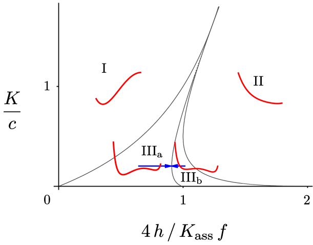
Figure 2: Typical form of the effective potential $V_{\psi,h}(\varphi)$ (red curves) in different parameter regions (cf. supplementary text of Ref. [11]). Region I: one equilibrium point $\varphi_{-}<c$; Region II: one equilibrium point $\varphi_{+}=c$; Region III_a: one stable equilibrium $\varphi_{-}<c$ and one metastable equilibrium $\varphi_{+}=c$. Region III_b: same as III_a, but now $\varphi_{+}=c$ is stable and $\varphi_{-}$ is metastable. The phase coexistence curve separating III_a from III_b is defined by the condition $V_{\psi,h}(\varphi_{-})=V_{\psi,h}(\varphi_{+})$. Arrows show the direction of the dynamic drift towards the phase coexistence curve.

In the present problem, the volume concentration $f$ of free enzymes varies in time (but not in space). More information about its values can be gotten in the limit (realized for small membrane diffusivities and large times) when the interface between the $\varphi_{+}$ and the $\varphi_{-}$ phase is much smaller than the typical domain size, allowing us to use the so-called thin wall approximation. Then, the value of $f$ is simply linked (see B) to the area covered by the $\varphi_{-}$ phase:

$$f(t)-f(\infty) \propto \int_{S}\varphi(\mathbf{r},t)\mathrm{d}\mathbf{r}-\int_{S}\varphi(\mathbf{r},\infty)\mathrm{d}\mathbf{r}\propto\psi(t)$$

showing that the metastability degree is proportional to the excess fraction of free cytosolic $u$ enzymes with respect to their value at equilibrium. The presence of this global feedback mechanism corresponds to Property 3.

The present situation is closely reminiscent of the decay of the uniform, metastable state of a supersaturated solution with the formation of precipitate grains [19]. In that case, the metastability degree is proportional to the excess solute concentration with respect to its equilibrium value. The main difference with the present case is that in the case of precipitation, the density field $\varphi$ is locally constrained by the law of particle conservation [7], and its evolution is described by Model B of Ref. [15], instead than by model A.

5 Phase separation kinetics

In polarization experiments cells are exposed to uniform or gradient distributions of attractant factors and polarize either spontaneously, or in the direction of the attractant gradients [38]. The properties of the model free energy described in the previous Section and numerical simulations of a model system [11] suggest that the introduction of an external attractant distribution moves the system in a region of bistability, where the uniform phase realized at initial time becomes metastable and germs of a new phase are nucleated. Depending on the way the system is prepared at initial time, the metastable phase can be either a $\varphi^{+}$ rich or a $\varphi^{-}$ rich phase.

The process of decay of a metastable state in physical systems described by systems of equations similar to (3, 4) has been extensively studied in the framework of the theory of first-order phase transitions [19, 7]. The process passes through successive stages of nucleation, coarsening, and coalescence (Fig. 3). In the first stage, approximately circular germs of the new, stabler phase are produced in the sea of the metastable phase by random fluctuations, or by the presence of nucleation centers. In the second stage, a process of coarsening is observed, where larger domains of the new phase grow at the expense of smaller ones, the average size of domains grow, and the average number of domains decreases. In a finite system, the process is concluded when a state of phase coexistence is reached. In this final state, the two phases are in equilibrium and are polarized in two large complementary domains.

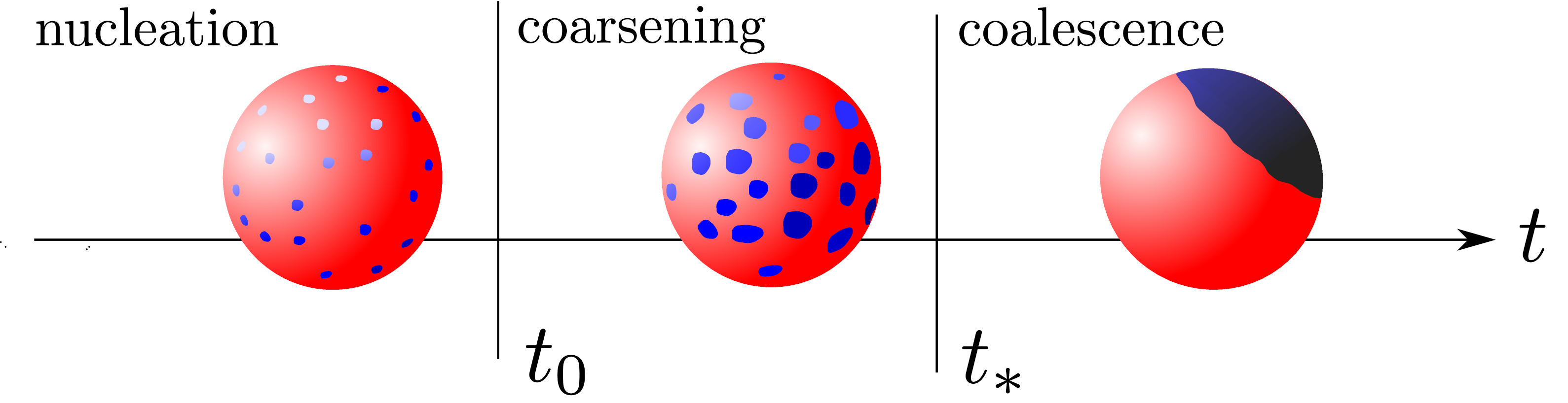
Figure 3: Stages of polarization kinetics.

For our purposes, a detailed knowledge of the initial, nucleation stage  is not necessary, as long as its characteristic time $t_{0}$ is so fast that a large number of germs of the new phase is nucleated all over the cell surface, well before the coarsening stage starts .

To understand the subsequent, coarsening state we have to focus on the laws by which the domains of the new phase either grow or shrink.

We consider here the case when the new phase is a minority phase, so that we can restrict our consideration to approximately circular domains, which are dominating because they minimize the linear tension between the two phases. For simplicity, we shall also restrict to domains which are small enough that membrane curvature may be neglected.

An approximate equation for the growth of a circular domain of size $r$ may be derived from (3) in the thin wall approximation. Inserting the approximate propagating solution $\varphi(\mathbf{R},t)=\phi(R-r(t))$ (Fig. 4a) for the radial domain profile in (3) and integrating over $S$ we get

$$\frac{\partial\mathcal{F}_{\psi,h}[\phi]}{\partial r} = -\frac{\partial Q}{\partial\dot{r}}+\xi^{\prime}$$ (5)

where

$$Q = \frac{\dot{r}^{2}}{2}\int_{S}(\phi^{\prime})^{2}\mathrm{d}\mathbf{R}$$

is a dissipation function [17] and $\xi^{\prime}$ is a noise term.

For a circular domain of radius $r$, $Q\simeq\gamma\pi r\dot{r}^{2}$, where

$$\gamma = \int_{0}^{\infty}(\phi^{\prime})^{2}\mathrm{d}R=\int_{\varphi_{-}}^{\varphi_{+}}\sqrt{2V_{\psi,h}(\phi)/D}\mathrm{d}\phi$$

is a kinetic coefficient [7]. On the other hand the effective free energy for a circular domain or radius $r$ is  [7]:

$$\mathcal{F}_{\psi,h} = 2\pi\sigma r-\pi r^{2}\psi$$ (6)

where $\sigma=D\gamma$ is a linear tension.

From (5, 6) we get the following approximate equation for the growth of a circular domain of size $r$:

$$\gamma\dot{r} = \psi-\frac{\sigma}{r}+\xi$$ (7)

where $\xi$ is a noise term.

Eq. (7) shows that domains smaller than the critical radius

$$r_{c} = \frac{\sigma}{\psi}$$

are mainly dissolved by diffusion, while germs with $r>r_{c}$ mainly survive and grow because of the overall gain in free energy (Fig. 4b).

a

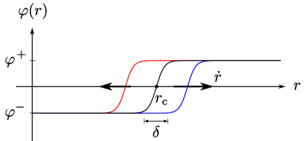
b

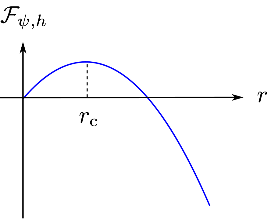
Figure 4: a: Radial profile of a growing ($r>r_{c}$) and a shrinking ($r<r_{c}$) circular domain of the $\varphi_{-}$ phase in the sea of the $\varphi_{+}$ phase. The $\varphi_{+}$ and the $\varphi_{-}$ phase are separated by a diffusive interface of thickness $\delta$. b: Qualitative graph of the effective free energy of a circular domain of size $r$. Domains larger than $r>r_{c}$ tend to grow because the energetic gain due to the surface term $\pi r^{2}\psi$ overcompensate the loss due to a longer interface. The converse happens for domains with $r<r_{c}$.

During the nucleation stage the noise term produces a population of germs of the new phase of size close to

$$r_{0} \sim r_{c}\sim\delta$$

in a characteristic time $t_{0}$. For domains with $r>r_{c}$ the noise term in (7) may be neglected and domain growth is an almost deterministic process.

It is interesting to estimate $r_{0}\sim\delta$ in terms of observable parameters. The thickness $\delta$ can be estimated as

$$\delta \sim \sqrt{D/b}$$

where $b$ is the potential barrier separating the two phases [7]. The height of the potential barrier may in its turn be estimated dimensionally from (B) as $b\sim k_{\mathrm{cat}}hc$, giving

$$r_{0} \sim \delta\sim\sqrt{\frac{D}{k_{\mathrm{cat}}}\frac{c}{h}}$$ (8)

Using realistic parameter values ($D\sim 1\mu m^{2}/s$, $k_{\mathrm{cat}}\sim 1s^{-1}$, $c/h\sim 10$) we get $r_{0}\sim 1\mu m$.

6 The coarsening stage

When domains of the new phase occupy an appreciable fraction of the membrane surface $S$ a coarsening stage sets on. Domain growth makes the degree of metastability $\psi$ decrease and renders further growth of the new phase more and more difficult. The critical radius $r_{c}$ grows with time, so that domains that earlier had size larger than $r_{c}$ become undercritical and shrink, and larger domains grow at the expense of smaller ones. In a large system $r_{c}$ soon becomes the main length scale in the problem, leading to the appearance of a scaling distribution of domains of size $r$.

The population of coarsening domains of size $r$ can be described in terms of the size distribution function $n(r,t)$, such that $n(r,t)\Delta r$ is the average number of domains with size comprised between $r$ and $r+\Delta r$, and the total number of domains at time $t$ is given by

$$N(t) = \int_{0}^{\infty}n(r,t)\mathrm{d}r$$

The time evolution of $n(r,t)$ implied by (7) is described by a standard Fokker-Planck equation [36]. If we restrict our consideration to supercritical domains we can neglect the diffusive part of the Fokker-Planck equation since for them the noise term $\xi$ is negligible.  This means that the stochastic nature of the problem enters mainly in the formation of the initial distribution of germ sizes $n(r,t_{0})$, while for $r>r_{c}$ the time evolution of $n(r,t)$ is dictated by the deterministic part of (7). Thus, we are left with the following kinetic equation:

$$\gamma\frac{\partial n(r,t)}{\partial t}+\frac{\partial}{\partial r}\left[\left(\psi(t)-\frac{\sigma}{r}\right)n(r,t)\right] = 0$$ (9)

Eq. (9) contains the unknown function $\psi(t)$, and is therefore not closed. We obtain a closed system by complementing (9) with the asymptotic law

$$\psi(t) \propto A_{\infty}-\int_{0}^{\infty}\pi r^{2}n(r,t)\mathrm{d}{\color[rgb]{0,0,0}}r$$ (10)

obtained from (4) in the thin wall approximation. Here

$$A_{\infty} = \int_{0}^{\infty}\pi r^{2}n(r,\infty)\mathrm{d}{\color[rgb]{0,0,0}}r$$

is the area occupied by the new phase at equilibrium.

For large times a scaling distribution of domain sizes can be found explicitly (D and Fig. 5):

$$n(r,t)\mathrm{d}r = \frac{CA_{\infty}}{r_{c}^{2}}p(r/r_{c})\mathrm{d}(r/r_{c}),\hskip 20.00003pt\psi(t)=\frac{\sigma}{r_{c}}$$

$$r_{c} \equiv r_{c}(t)=r_{0}(t/t_{0})^{1/2}$$ (11)

where

$$p(\rho) = {\color[rgb]{0,0,0}\frac{8\mathrm{e}^{2}\rho}{(2-\rho)^{4}}\exp\left(-\frac{4}{2-\rho}\right)},\hskip 20.00003ptt_{0}=\frac{2\gamma r_{0}^{2}}{\sigma},$$ (12)

where $r_{0}$ is the characteristic domain size at the beginning of the coarsening stage and $C\simeq 0.11$.

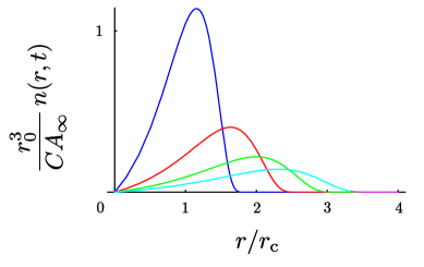
Figure 5: Time evolution of the selfsimilar domain size distribution $n(r,t)$ ($t/t_{0}=1,2,3,4$).

The total number of domains decreases in time due to the evaporation of small domains. Using the explicit solution (11, 12), we easily find:

$$N(t)=\int_{0}^{\infty}n(r,t)\mathrm{d}r = \frac{CA_{\infty}}{r_{c}^{2}}=\frac{CA_{\infty}/r_{0}^{2}}{t}$$

Similarly, it is possible to compute explicitly the value of the average domain size, which is found to coincide exactly with the critical radius:

$$\langle r\rangle = r_{c}$$

7 Spontaneous and gradient-induced polarization

The coarsening theory exposed in the previous Section allows to deduce a simple scaling law for the time needed for spontaneous cell polarization.

If the cell has size $R$, the growth of domains according to (11) comes to a stop at the time $t_{\ast}$ when the average patch size $\langle r\rangle$ becomes of the order of the cell size $R$. From (11) we get

$$t_{\ast} \sim t_{0}\left(R/r_{0}\right)^{2}$$

At the end of the process the cell is polarized in a random direction. The actual direction of polarization is the result of the initial random unbalance in the germ distribution.

The typical time for random polarization is of the order of $10^{3}\,\mathrm{s}$ [12]. Together with the estimate (8) this gives $t_{0}\sim 10\,\mathrm{s}$.

Let us now consider the case where a source of external attractant is present at some distance from the cell, in such a way that a gradient of external attractant is created by diffusion close to the cell surface (Fig. 6).

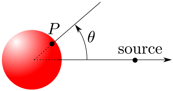
Figure 6: Geometry of stimulation of a cell by an external source of attractant.

The inhomogeneity in the distribution of attractant induces a similarly inhomogeneous distribution of activated enzymes $h$. This way, the degree of metastability $\psi$ takes on different values on different points of the cell surface.

If the cell membrane has a nearly spherical form and a radius $R$ much smaller than the characteristic scale of the attractant distribution, and if the gradient component of the activation field is small with respect to the background component on the scale $R$, the metastability degree $\psi$ at the beginning of the coarsening process may be written as the sum of a uniform component $\psi$ and a small space-dependent perturbation:

$$\psi+\delta\psi\hskip 20.00003pt\mathrm{with}\hskip 20.00003pt\delta\psi=-\epsilon\psi_{0}\cos\theta$$

where $\psi_{0}$ is the value of the uniform component at the beginning of the coarsening process and $\epsilon$ is the relative gradient on the scale $R$. The perturbation modifies the equation of domain growth (7) as follows:

$$\gamma\dot{r} = \psi-\frac{\sigma}{r}-\epsilon\psi_{0}\cos\theta+\xi$$ (13)

where $\theta$ is an azimuthal angle defined in Fig. 6.

The uniform component $\psi$ varies in time together with the (approximately) uniform concentration of $u$ molecules in the cell volume. On the other hand, the perturbation $\delta\psi$ is constant in time, but not uniform in space, being proportional to the external attractant distribution.

As long as $\epsilon\psi_{0}\ll\psi$, the effect of the perturbation is negligible, so domain growth proceeds according to the law (11) and the uniform component $\psi$ decays as $t^{-1/2}$.

In a large cell there is a crossover time $t_{\epsilon}$ when the perturbation becomes of the same order of the uniform component:

$$\psi(t_{\epsilon}) = \epsilon\psi_{0}$$

Using the scaling law (11) we get

$$t_{\epsilon} = \frac{t_{0}}{\epsilon^{2}}$$

After $t_{\epsilon}$ domain growth enters in a new stage, where the growth becomes anisotropic. Domains in the front and back of the cell get different average sizes (Fig. 7).

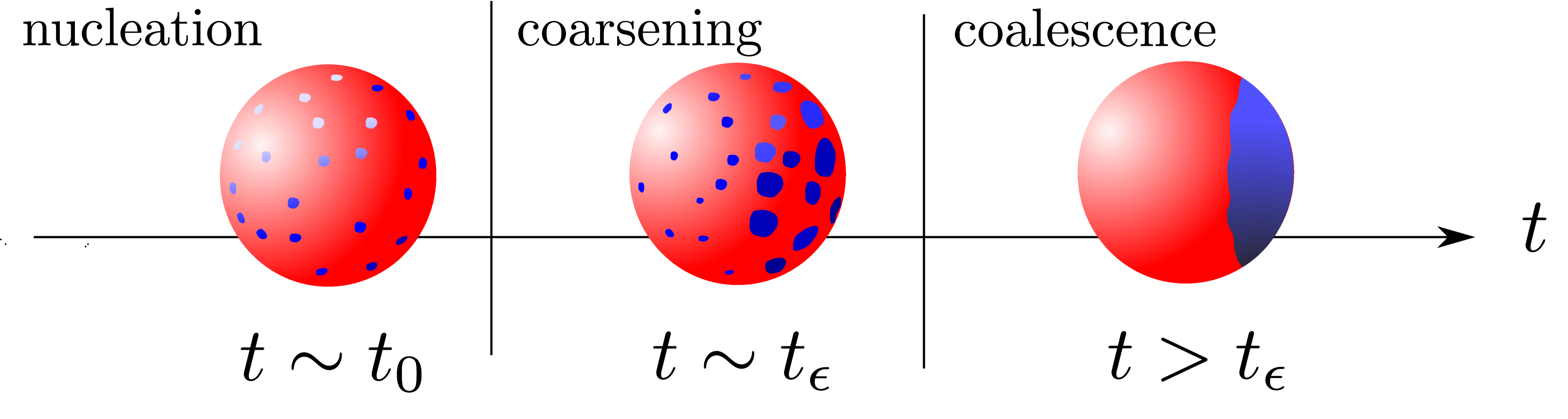
Figure 7: The crossover time $t_{\epsilon}$ separates an initial stage of isotropic coarsening from a final stage when domains evaporate from the back of the cell and condense in the front.

Indeed, for $t>t_{\epsilon}$ the leading term in (13) is the perturbation $\epsilon\psi_{0}\cos\theta$, implying that in the region closer to the source of the perturbation ($\cos\theta>0$) the $\varphi_{-}$ phase evaporates, and in the region away from the source ($\cos\theta<0$) it condenses. At the end of the process,  complete polarization is realized (Fig. 7). In this final stage domains grow approximately linearly in time, thus the total time $t_{\epsilon}^{\prime}$ to reach polarization is still a quantity of order $t_{\epsilon}$ (using definition (14) from the next Section it can be estimated as $\frac{1}{2}\left(1+\epsilon/\epsilon_{\mathrm{th}}\right)t_{\epsilon}$).

The above scheme is valid as soon as the initial nucleation time $t_{0}$ is significantly smaller than $t_{\epsilon}$, an assumption which is compatible with the observation of real [25] and numerical [11] experiments.

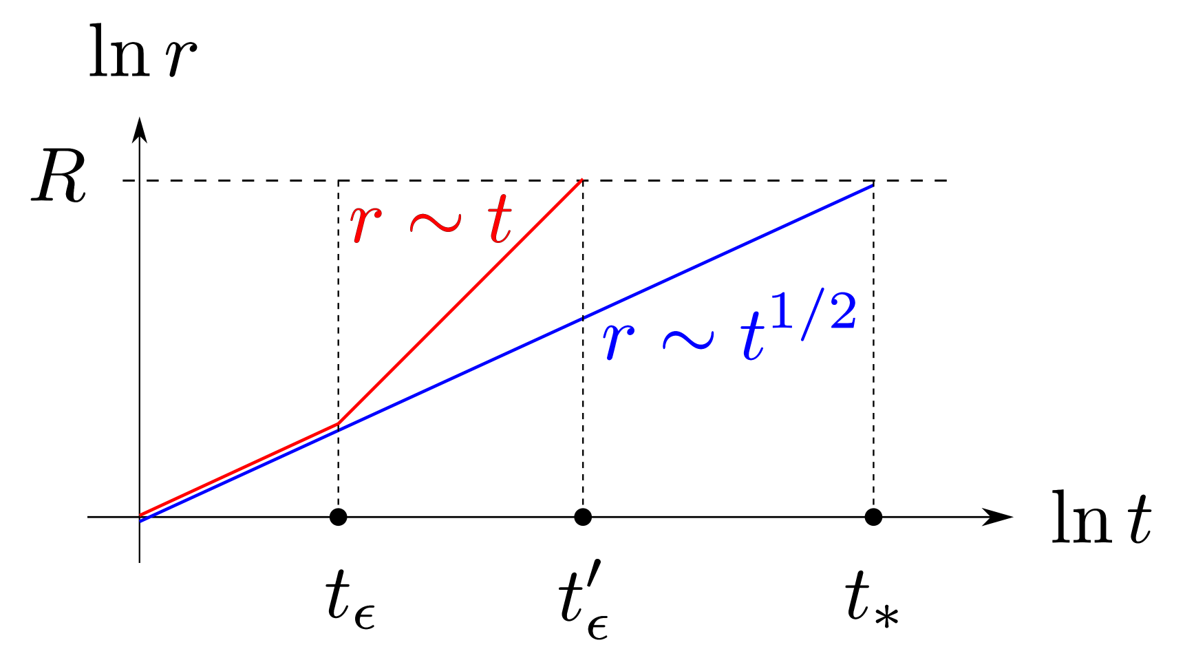
Figure 8: Dynamic mechanism of gradient sensing. In the presence of a gradient (red) domain sizes grow initially as $t^{1/2}$. After the crossover time $t_{\epsilon}$ they grow linearly in time and the cell polarizes in the direction of the gradient (see also Fig. 7). In the absence of a gradient (blue) the $t^{1/2}$ growth goes on until the cell polarizes in a random direction.

8 Gradient sensitivity

The second stage of domain evolution described in the previous Section occurs only if $t_{\ast}>t_{\epsilon}$. Otherwise, the presence of a gradient of attractant becomes irrelevant and only the stage of isotropic domain growth actually occurs. This condition implies that a smallest detectable gradient exists, such that directional sensing is impossible below it. The threshold value $\epsilon_{\mathrm{th}}$ for $\epsilon$ is found by the condition $t_{\epsilon}=t_{\ast}$. Since the product $\psi r_{c}$ is a time-independent constant, we can simply compare its value at initial and final time when $\epsilon=\epsilon_{\mathrm{th}}$, obtaining that the threshold detectable gradient is

$$\epsilon_{\mathrm{th}} = \frac{r_{0}}{R}$$ (14)

Using the estimates from Sections 5 and 7, and the typical value $R\sim 10\,\mu\mathrm{m}$, we get $\epsilon\sim 10\%$, a value which is compatible with the observations [33].

An interesting speculation is that the bound (14) may explain why spatial directional sensing was developed only in large eukaryotic cells and not in smaller prokaryotes, whose directional sensing mechanisms rely instead on the measurement of temporal variations in concentration gradients [3]. By solving (14) in terms of the size $R$ we get the following bound for the size of a cell which may be able to sense a relative gradient $\epsilon$:

$$R > \frac{r_{0}}{\epsilon}$$

Our bound goes in the same direction as the size criterion formulated in [5], but it’s independent of it, since the criterion of Ref. [5] is based on estimates of signal-to-noise ratios, while our bound stems from the intrinsic properties of polarization dynamics.

9 External fluctuations

One may wonder whether a cell may become polarized by transient gradients produced by a spontaneous fluctuation in the external distribution of attractant molecules, or fluctuations in receptor-ligand binding, as has been suggested in the literature [18]. Since eukaryotic cells typically carry 10⁴–10⁵ receptors for attractant factors, one expects spontaneous fluctuations in the fraction of activated receptors to be of the order of 10², a value which is comparable to observed anisotropy thresholds. However, to actually produce directed polarization the fluctuation should sustain itself for several minutes, i.e. for a time comparable to the characteristic polarization time (such as $t_{\epsilon}$ ). Such an event has very low probability of being observed since the correlation time of the fluctuations determined by attractant diffusion at the cell scale and the characteristic times of receptor-ligand kinetics are much less than the polarization time. Indeed, the diffusion time is $\sim 1\,$s at the typical cell size $10\,\mu$m, and the characteristic times of receptor-ligand kinetics are also $\sim 1\,$s (see online supporting information to Ref. [33]). Therefore, the direction of cell polarization in the case of a homogeneous distribution of attractant can only be determined by the inhomogeneity in the initial distribution of the positions of PIP2-rich germs produced by thermal fluctuations.

10 Conclusions

By using standard statistical mechanical methods we have shown that the dynamics of signaling domains in cell polarization is independent on the nature of the signaling molecules and the values of kinetic rate constants, as long as some very general conditions are met:

1. Timescale separation allows to describe the polarization process in terms of a single concentration field of signaling molecules on the cell membrane .

2. The underlying chemical reaction network is bistable.

3. A global feedback mechanism drives the system towards phase coexistence.

4. The cell is sufficiently larger than the size of nucleating germs of the new phase.

These conditions allow the cell to work as a detector of slight gradients of external stimulation gradients.

The property of universality arising from our analysis cannot be underestimated. Presently, several efforts are made to understand the dynamical behavior of living beings starting from microscopic informations provided by molecular biology. However, these informations are mostly incomplete and poorly quantitative, and theories that depend in a sensitive way on them are likely to be of little utility. But if some behavior happens to be universal, a consistent physical theory of it may be built, which can be compared to experiments.

The universal properties of cell polarization emerge from properties of domain growth which have been extensively studied in first-order phase transitions [7]. The similarity of the two problems follows from the fact that fast degrees of freedom of chemical kinetics are in approximate equilibrium with slower degrees of freedom, which can be described by means of an effective free energy functional. It is worth observing that in the biological system studied here, there is no direct interaction between signaling molecules, similar to the one observed in solid state system such as binary alloys, but only an effective interaction mediated by enzyme activity, binding, unbinding and diffusion processes.

Our theoretical scheme allows to shed light on some non trivial questions, such as the mechanism of directional sensing and the effect of random fluctuations of the medium on the polarization process. Random polarization appears as the result of the intrinsic stochasticity of the process of domain nucleation and not of random fluctuations of the medium. Random and gradient-induced polarization appear as the two sides of a same coin. Our scheme provides an explanation of why spatial directional sensing is not observed in the small prokaryotic cells, and provides asymptotic estimates for polarization times and threshold detectable gradients.

An important component of our picture is the existence of a global coupling of the degree of metastability to the state of the system [12, 10]. The constrained phase-ordering dynamics tunes the system towards phase coexistence, similarly to what happens in the case of a precipitating supersaturated solution. The global control allowing self-tuning to phase-coexistence is realized by shuttling of enzymes from the cytosol to the cell membrane and backwards.

Some of the features that we have observed in cell polarization have been considered in previous works, such as the fact that equations of the form (1) are relevant for the description of systems of bistable chemical reactions [29, 36], and that global couplings in activator-inhibitor reaction-diffusion systems may lead to the formation of stable spatiotemporal patterns [14, 30]. The peculiar properties of this kind of systems have led to the use of the term of excitable or active media.  Using this same language, we can say that the cell membrane acts as an active medium responding to the stimulation with the formation of domains of a new phase. Our work proposes that directional sensing results from the peculiar, universal features of the phase-ordering dynamics of these domains.

From a biological point of view, the universality of the polarization process allows the cell to behave in a robust, predictable way, independent on microscopic peculiarities such as the precise values of reaction rates and diffusion constants.

We first proposed that chemotactic cell polarization may result from the simple ingredients of bistability induced by a positive local feedback loop in a signaling network and global control induced by shuttling of enzymes between the cytosol and the membrane in our previous works [11, 12, 9]. Other authors have proposed similar models, either independently [32] or subsequently [21] (a review of models of chemotactic polarization can be found in Ref. [16]). Some of these models try to take into account computationally the interactions of a large numbers of chemical factors, while retaining the essential role of a feedback loop as generator of a phase-separation instability. However, most of the reaction rates that should be provided to perform such computations are known with very poor accuracy. Our framework suggests however that such a detailed description may be not necessary, as long as properties a),…,d) are met.

Aspects of the bistable mechanism of eukaryotic polarization firstly introduced in Ref. [11] (supporting material) have been considered in recent papers [6, 22] as relevant to polarization phenomena. A similar mechanism, out of the bistability region, has been proposed to explain intermittent polarization in budding yeast [4]. These works suggest that the combination of bistability and global control [11, 12] is providing a useful paradigm for the understanding of cell polarization phenomena.

Acknowledgments

We thank Guido Serini for many inspiring discussions. This research was supported in part by the National Science Foundation under Grant No. NSF PHY05-51164.

Appendix A Lattice gas description of cell polarization

The signaling molecules PIP2 and PIP3 are different phosphorylation states of the phosphatidylinositol molecule, i.e., they carry a different number of phosphate groups attached (2 and 3, respectively). Enzymes which catalyze phosphorylation of their substrate, i.e. the addition of a phosphate group, are called kinases, while dephosphorylating enzymes are called phosphatases.

It is natural to visualize the state of a chemical system such as the one described in Fig. 1 in terms of two families of classical spins on a twodimensional lattice, taking on values -1 (PIP2, PTEN), 0 (an empty site), +1 (PIP3, PI3K) [10]. Taking into account fast cytosolic diffusion, the enzyme family becomes slaved to the substrate family [10].

In this lattice-gas description the existence of a cytosolic enzymatic reservoir exchanging enzymes with the cell membrane is represented by a chemical potential for enzyme creation and destruction (actually, adsorption and desorption to/from the cell membrane), globally coupled to the lattice configuration [10].

The PIP2 and PIP3 molecules constitute approximately 1% of the total number of membrane phospholipids, and the number of PI3K and PTEN enzymes are at least one order of magnitude lower, thus, both the substrate and the enzyme population should be thought as diluted gases.

Two-state (or multistate) molecules such as PIP2 and PIP3 are all but an exception in cell biology. Another example is given by small GTPases, such as the Cdc42 molecule involved in the polarization of budding yeast, which can be found either in the activated GTP state or in the deactivated GDP state. The switch between the two phosphorylation states is catalyzed by a couple of activating (GEF) and deactivating (GAP) enzymes [2].

Appendix B Mean-field equations for eukaryotic polarization

We derive here mean-field equations for eukaryotic polarization using standard methods of chemical kinetics, including Michaelis-Menten saturation terms for the enzymatic components . We make use of the fact that the diffusivity $D_{\mathrm{vol}}$ of $u$ enzymes in the cytosol is much faster than the diffusivity $D$ of $\varphi$ molecules on the cell membrane: this fact allows to considerably reduce the number of dynamical degrees of freedom.

We describe the macroscopic state of the cell using surface concentration fields of membrane-bound molecules (Fig. 1) and the volume concentration field $f\equiv u_{\mathrm{free}}$ of free $u$ enzymes.

The chemical kinetic equations for the signaling network of eukaryotic polarization are:

$$\partial_{t}\varphi^{+} = D\nabla^{2}\varphi^{+}-k_{\mathrm{c}\mathrm{at}}\frac{u\varphi^{+}}{K+\varphi^{+}}+k_{\mathrm{\mathrm{cat}}}\frac{h\varphi^{-}}{K+\varphi^{-}}$$ (15)

$$\partial_{t}\varphi^{-} = D\nabla^{2}\varphi_{-}+k_{\mathrm{c}\mathrm{at}}\frac{u\varphi^{+}}{K+\varphi^{+}}-k_{\mathrm{c}\mathrm{at}}\frac{h\varphi^{-}}{K+\varphi^{-}}-\partial_{t}u$$ (16)

$$\partial_{t}u = k_{\mathrm{a}\mathrm{ss}}f\varphi^{-}-k_{\mathrm{{diss}}}u$$ (17)

$$\partial_{t}f = \nabla\cdot(D_{\mathrm{vol}}\nabla f),\hskip 20.00003pt\hskip 20.00003pt$$ (18)

They must be complemented with the boundary condition

$$J \equiv D_{\mathrm{vol}}\frac{\partial f}{\partial\mathbf{n}}=\partial_{t}u$$ (19)

where $\partial/\partial\mathbf{n}$ is the derivative along the outward normal to the membrane surface $S$. Condition (19) expresses the fact that the flux of $u$ enzymes leaving the cytosolic volume equals the flux of enzymes being bound to the cell membrane.

For simplicity, we consider here identical catalytic, association and dissociation rates ($k_{\mathrm{cat}}$, $k_{\mathrm{ass}}$, $k_{\mathrm{diss}}$) and Michaelis-Menten constants $K$ for the $\varphi^{+}\rightarrow\varphi^{-}$ and $\varphi^{-}\rightarrow\varphi^{+}$ processes. This is compatible with existing information about these processes, suggesting that reaction rates differ by factors of order 1 [11] and allows to easily study the equations analytically.

Typical values for surface and cytosolic diffusivity are $D\sim 1\mu m^{2}/s$, $D_{\mathrm{vol}}\sim 10\mu m^{2}/s$ [11]. Typical values for rate constants are: $k_{\mathrm{cat}}\sim k_{\mathrm{diss}}\sim 1s^{-1}$, $k_{\mathrm{ass}}\sim 0.05s^{-1}\mathrm{nM}^{-1}$; for the total number of $\varphi^{+}$ and $\varphi^{-}$ molecules, and the total number of $u$ and $h$ enzymes: $N_{\varphi}\sim 10^{6}$, $N_{u}\sim N_{h}\sim 10^{4}$–$10^{5}$. Observe that $N_{u}/N_{\varphi}\ll 1$.

The usual definition of macroscopic fields such as $u$ is as follows. For each point $\mathbf{r}$ in space we choose a volume $v$ centered in $\mathbf{r}$, containing $n(v)$ molecules, and we compute concentrations as $u(\mathbf{r})=\lim_{v\rightarrow 0}n(v)/v$. This implies that the number of molecules of the relevant chemical factors is so large that $v$ can be chosen much smaller than the size of the system, but large enough that the resulting field $\varphi(\mathbf{r})$ is approximately continuous. This hypothesis is not always acceptable, since enzymatic molecules are present in the cell in very small numbers. We shall therefore assume that real concentrations are described as the sum of an average part $u$, described by mean field equations of the kind (15–19), and a fluctuating part $\delta u$ taking into account both the discrete character of the concentration field and thermal disorder. The fluctuations $\delta u$ due to random adsorption and desorption processes are at the origin of the noise term $\Xi$ in (3) (see C).

Since enzyme diffusion in the cytosol is faster than phospholipidic diffusion on the membrane, during the characteristic times of the dynamics of membrane-bound factors, $f(\mathbf{r},t)$ relaxes to the approximately uniform value

$$f(t) = f_{0}-\frac{1}{V}\int_{S}u_{-}(\mathbf{r},t)\mathrm{d}\mathbf{r}$$ (20)

where $f_{0}=N_{u}/V$, while $u$ relaxes to the local equilibrium value

$$u = K_{a\mathrm{ss}}f\varphi^{-}$$ (21)

where $K_{\mathrm{ass}}=k_{\mathrm{ass}}/k_{\mathrm{diss}}$.

On the other hand, by summing (15) and (16) we get

$$\partial_{t}\left(\varphi_{+}+\varphi_{-}\right) = D\nabla^{2}(\varphi_{+}+\varphi_{-})-\partial_{t}u_{-}$$ (22)

Since $N_{u}/N_{\varphi}\ll 1$ we neglect the term $\partial_{t}u$. Then, (22) shows that the sum $c=\varphi^{+}+\varphi^{-}$ tends to be approximately uniform and constant in time.

By subtracting (15) and (16) and introducing the difference concentration field $\varphi=\varphi^{+}-\varphi^{-}$ we get

$$\partial_{t}\varphi = D\nabla^{2}\varphi-k_{\mathrm{cat}}\frac{2u(c+\varphi)}{2K+c+\varphi}+k_{\mathrm{cat}}\frac{2h(c-\varphi)}{2K+c-\varphi}$$ (23)

and using the local equilibrium condition (21) we end up with

$$\partial_{t}\varphi = D\nabla^{2}\varphi-k_{\mathrm{cat}}K_{\mathrm{ass}}f\frac{c^{2}-\varphi^{2}}{2K+c+\varphi}+2k_{\mathrm{cat}}h\frac{c-\varphi}{2K+c-\varphi}$$ (24)

Only values $-c\leqslant\varphi\leqslant\varphi$ correspond to positive concentrations and are therefore physical.

From (24), (17) and (20) we get the following system:

$$\partial_{t}\varphi(\mathbf{r},t) = -\frac{\delta\mathcal{F}_{f,h}[\varphi]}{\delta\varphi(\mathbf{r},t)}$$ (25)

$$\dot{f}(t) = -V^{-1}k_{\mathrm{ass}}f(t)\int_{S}\varphi^{-}\mathrm{d}\mathbf{r}+k_{\mathrm{diss}}\left(f_{0}-f(t)\right)$$ (26)

where

$$\mathcal{F}_{f,h}[\varphi] = \int_{S}\left[\frac{1}{2}D\left|\nabla\varphi\right|^{2}+V_{f,h}(\varphi)\right]\mathrm{d}\mathbf{r}$$ (27)

$$V_{f,h}(\varphi) = \hskip 10.00002pt2k_{\mathrm{cat}}hc\left[-\phi-2\kappa\ln\left(2\kappa+1-\phi\right)\right]$$

$$+\frac{1}{2}k_{\mathrm{cat}}K_{\mathrm{ass}}fc^{2}[-\phi^{2}/2+\left(2\kappa+1\right)\phi$$

$$\left.-4\kappa(\kappa+1)\ln\left(2\kappa+1+\phi\right)\right]$$

and we make use of the nondimensional variables $\phi=\varphi/c$, $\kappa=K/c$.

The quantity $\mathcal{F}_{f,h}$ plays the role of a generalized free energy for the system, and can be used to study its approximate equilibria as long as the characteristic times of variation of $f$ are longer than the characteristic times of variation of the $\varphi$ field.

We are interested in parameter values such that (B) is bistable. In what follows we consider the case of constant and uniform activation field $h$, and constant $f$.

The critical points of the effective potential $V_{f,h}$ are

$$\phi_{-} = \kappa-\lambda/2-\sqrt{\left(\kappa-\lambda/2\right)^{2}-(\lambda-1)(2\kappa+1)}$$

$$\phi_{u} = \kappa-\lambda/2+\sqrt{\left(\kappa-\lambda/2\right)^{2}-(\lambda-1)(2\kappa+1)}$$

$$\phi_{+} = 1$$

where

$$\lambda = \frac{4h}{K_{a\mathrm{ss}}f}$$

The potential $V_{f,h}$ is bistable when the three critical points are all real and physical. In that case, (24) describes a dynamical system that may locally favor either a $\varphi^{-}$ rich or a $\varphi^{+}$ rich stable phase (Fig. 9).

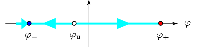
Figure 9: Eq. (24) describes a local flow towards either a $\varphi^{-}$ rich or a $\varphi^{+}$ rich stable phase.

The two roots $\phi_{-}<\phi_{u}$ are real if

$$\lambda < 2(3\kappa+1)-4\sqrt{\mathcal{\kappa}(2\mathcal{\kappa}+1)},\hskip 10.00002pt\lambda>2(3\mathcal{\kappa}+1)+4\sqrt{\mathcal{\kappa}(2\mathcal{\kappa}+1)}$$ (29)

The l.h.s. condition defines the right boundary of the bistability region of parameter space (Region III of Fig. 2).

The two roots are physical ($-1\leqslant\phi_{-}<\phi_{u}\leqslant 1$) when

$$\kappa \leqslant \frac{\lambda}{2-\lambda}\hskip 10.00002pt\mathrm{and}\hskip 10.00002pt\kappa\leqslant 1+\frac{\lambda}{2}$$ (30)

The l.h.s. condition defines the left boundary of the bistability region (Region III in Fig. 2). The inequality $\phi_{-}\geqslant-1$ on the other hand is always verified if $\lambda<2$.

The left and right boundaries of Region III meet in the triple point

$$\lambda = 1-\sqrt{5},\hskip 20.00003pt\kappa=(1+\sqrt{5})/2$$

So, the $\lambda$–$\kappa$ plane can be divided into three regions (Fig. 2 and supplementary text of Ref. [11]). In Region III, the system has to stable minima $\varphi_{+}$ and $\varphi_{-}$, separated by the unstable equilibrium $\varphi_{u}$. Outside Region III the potential has a single minimum, either rich in $\varphi^{-}$ (Region I) or rich in $\varphi^{+}$ (Region II).

Region III may be divided in two parts, depending on which phase is stabler. In Region III_a (Fig. 2) the stabler phase is $\varphi_{-}$, while in Region III_b it is $\varphi_{+}$. The two subregions are separated by the phase-coexistence curve $\psi\equiv V_{f,h}(\varphi_{+})-V_{f,h}(\varphi_{-})=0$, where the two stable equilibria $\varphi_{+}$ and $\varphi_{-}$ have the same energy.

Close to the phase coexistence curve $\psi$ is much smaller than the potential barrier separating the two minima. In this region

$$\psi \simeq 2k_{\mathrm{cat}}hc\left[\phi_{+}-\phi_{-}+2\kappa\ln\left(1+\frac{\phi_{+}-\phi_{-}}{2\kappa}\right)\right]\left(\frac{f}{f_{\infty}}-1\right)$$ (31)

where the factor $f/f_{\infty}-1$ represents the excess fraction of free $u$ enzymes at a given time, with respect to the equilibrium value.

Observe that an actual excess of free enzymes renders the $\varphi_{-}$ phase more stable, while a negative excess (a deficit) stabilizes the $\varphi_{+}$ phase.

If the $\varphi_{-}$ phase is the more stable one, it tends to occupy larger and larger regions of the cell surface, thus decreasing $f$ (cf. the quasi-equilibrium conditions (20) and (21)) and its own stability relative to the $\varphi_{+}$ phase.

A symmetric situation is encountered if $\varphi_{+}$ is the more stable phase at initial time.

Thus, the process of growth of any of the two phases decreases the metastability degree $\psi$ and drives the system towards a condition of phase-coexistence (i.e. towards a polarized state).

We may wonder whether uniform equilibrium states also exist, that may compete with polarized states. Looking for stable uniform equilibria $\varphi=\varphi_{-}$ in Region III_a gives the algebraic conditions

$$\lambda = \frac{-\phi^{2}+2\kappa\phi+(2\kappa+1)}{\phi+(2\kappa+1)}=2\frac{N_{h}}{N_{u}}\left[\left(1+\frac{2K_{\mathrm{ass}}}{VN_{\varphi}}\right)-\phi\right]$$ (32)

$$\varphi \leqslant 2\sqrt{\kappa(2\kappa+1)}-(2\kappa+1)$$ (33)

which may be studied graphically, showing that uniform equilibria are impossible in a large part of Region III, and in particular if

$$\kappa < \frac{1}{2}\hskip 10.00002pt\mathrm{and}\hskip 10.00002pt2\frac{N_{h}}{N_{u}}\left(1+\frac{2K_{\mathrm{ass}}}{VN_{\varphi}}\right)>1$$ (34)

Uniform equilibria do not exist in this region because the total number of $u$ enzymes is not large enough to stabilize a uniform $\varphi_{-}$ phase extended along the whole membrane surface.

Instead, uniform equilibria with $\varphi=\varphi_{+}$ exist, and correspond to configurations where all $u$ enzymes are free.

Appendix C Thermal and chemical noise

Up to this point we have neglected fluctuations in the number of membrane-bound enzymes, so that every local minimum of $V_{f,h}$ corresponds to a stable phase having an infinite lifetime. However, since the number of bound enzymes molecules in the real system fluctuates locally, the field $\varphi(\mathbf{r},t)$ should be seen as a stochastic field.

The fluctuations $\delta f$ around the equilibrium enzyme concentration $f_{\infty}$ in the volume $V$ due to membrane adsorption and desorption processes induce fluctuations $\delta u$ around the local equilibrium value (21) in the concentration of membrane-bound enzymes.

To derive quantitative relations we have to compute the encounter rates of a free $u$ particle fluctuating in the volume $V$ and a $\varphi_{-}$ binding site on the surface $S$.

The adsorption-desorption process can be described by a simple master equation [13]. Let us consider that a reservoir of volume $V$ contains a number $N^{\mathrm{free}}\leqslant N^{\mathrm{tot}}$ of molecules, which can be adsorbed and desorbed by a small surface element $\Sigma$ containing $N^{\mathrm{b.s.}}$ binding sites. One has the mean-field kinetic equation

$$\frac{\mathrm{d}}{\mathrm{d}t}N^{\mathrm{bound}} = k_{\mathrm{ass}}V^{-1}N^{\mathrm{b.s.}}N^{\mathrm{free}}-k_{\mathrm{diss}}N^{\mathrm{bound}}$$

which at equilibrium gives

$$N^{\mathrm{bound}} = \alpha N^{\mathrm{free}}=\frac{\alpha}{1+\alpha}N^{\mathrm{tot}}\hskip 20.00003pt\left(\alpha=K_{\mathrm{ass}}V^{-1}N^{\mathrm{b.s.}}\right)$$

Let $P_{N}$ be the probability to observe $N^{\mathrm{bound}}=N$, and $r^{\pm}_{N}$ the time rates of the processes $N\rightarrow N\pm 1$. Then the process is described by the master equation

$$\dot{P_{N}} = r^{+}_{N-1}P_{N-1}-(r^{+}_{N}+r_{N}^{-})P_{N}+r^{-}_{N+1}P_{N+1}$$

which has the stationary solution

$$P_{N} = \prod_{j=0}^{N-1}\frac{r^{+}_{j}}{r^{-}_{j+1}}P_{0}$$

where $P_{0}$ is a normalizing factor. Letting

$$r^{+}_{N} = c\,k_{\mathrm{ass}}(N^{\mathrm{tot}}-N),\hskip 20.00003ptr^{-}_{N}=k_{\mathrm{diss}}N$$

one finds a binomial distribution with

$$\langle N^{\mathrm{bound}}\rangle = {\color[rgb]{0,0,0}\frac{\alpha N^{\mathrm{tot}}}{1+\alpha}}=\alpha N^{\mathrm{free}}$$

$$\langle\left(N^{\mathrm{bound}}\right)^{2}\rangle-\langle N^{\mathrm{bound}}\rangle^{2} = {\color[rgb]{0,0,0}\frac{\alpha N^{\mathrm{tot}}}{\left(1+\alpha\right)^{2}}}=\frac{N^{\mathrm{bound}}N^{\mathrm{free}}}{N^{\mathrm{tot}}}$$

By identifying $f=N^{\mathrm{free}}/V$ in (21) we can model the adsorption-desorption noise with a Gaussian noise term $\Xi$ with zero mean and the correct variance:

$$\langle\Xi(\mathbf{r},t)\Xi(\mathbf{r}^{\prime},t^{\prime})\rangle = 2\Gamma\delta(\mathbf{r}-\mathbf{r}^{\prime})\delta(t-t^{\prime})$$

where

$$\Gamma = \frac{k_{\mathrm{diss}}}{k_{\mathrm{cat}}}\frac{\varphi^{+}}{K+\varphi^{+}}\frac{f}{f_{0}}(K_{\mathrm{ass}}f\varphi^{-})$$

Appendix D Scale invariant size distribution

In the domain coarsening stage described in Section 6, the characteristic size $r_{c}(t)$ of domains grows with time, and soon becomes the largest scale, so that a scaling distribution of domain sizes arises. In the asymptotic regime (for large times) it is possible to derive a self similar solution of the system of equations (9, 10):

$$\gamma\frac{\partial n(r,t)}{\partial t}+\frac{\partial}{\partial r}\left[\left(\psi(t)-\frac{\sigma}{r}\right)n(r,t)\right] = 0$$ (35)

$$\psi(t)\propto A_{\infty}-\int_{0}^{\infty}\pi r^{2}n(r,t)\mathrm{d}{\color[rgb]{0,0,0}}r \rightarrow 0\hskip 20.00003pt\mathrm{for}\hskip 20.00003ptt\rightarrow\infty$$ (36)

We start by looking for a solution in the form

$$n(r,t) = \left[r_{c}(t)\right]^{k}g(r/r_{c}(t))$$ (37)

It is easy to verify that $k$ must be given the value $-3$ in order that (36) may attain its asymptotic limit.

Substituting (37) in (35), reexpressing the result in terms of the nondimensional variable

$$\rho = r/r_{c}$$

and balancing terms in the resulting equation, we find that an asymptotic solution for large times may exist only if

$$\psi(t) = \frac{\sigma}{r_{c}(t)},\hskip 20.00003ptr_{c}(t)=r_{0}\left(t/t_{0}\right)^{1/2}$$

and

$$\left[{\color[rgb]{0,0,0}-\sigma\rho+\sigma\rho^{2}-\frac{1}{2}\frac{\gamma r_{0}^{2}}{t_{0}}\rho^{3}}\right]g^{\prime}(\rho)+\left[{\color[rgb]{0,0,0}\sigma-\frac{3}{2}\frac{\gamma r_{0}^{2}}{t_{0}}\rho^{2}}\right]g(\rho) = 0$$ (38)

A smooth, positive, normalizable solution of (38) may be found only when two of the poles of $g^{\prime}(\rho)/g(\rho)$ coalesce, which gives

$$t_{0} = \frac{2\gamma r_{0}^{2}}{\sigma}$$ (39)

and finally 

$$g(\rho) = \left\{\begin{array}[]{ll}CA_{\infty}\frac{8\mathrm{e}^{2}\rho}{(2-\rho)^{4}}\exp\left(-\frac{4}{2-\rho}\right)&\mathrm{for}\hskip 10.00002pt0\leqslant\rho\leqslant 2\\ 0&\mathrm{elsewhere}\end{array}\right.$$

with

$$C = \frac{1}{4\pi[1+2\mathrm{e}^{2}\mathrm{Ei}(-2)]}\simeq 0.11$$

a normalization factor and Ei the exponential integral function [1] .

The resulting size distribution function is peaked around $r_{c}\sim t^{1/2}$ and there are no domains with sizes larger than $2r_{c}$ (Fig. 5).

The physical meaning of (39) can be understood by rewriting the deterministic part of the equation of domain growth (7) using $\rho$:

$$\frac{\gamma r_{c}^{2}}{\sigma}\dot{\rho} = -\frac{\frac{\gamma r_{0}^{2}}{2\sigma t_{0}}\rho^{2}-\rho+1}{\rho}$$ (41)

The analysis of the fixed points of (41) shows that when condition (39) is not satisfied, either the total domain area grows to infinity, or shrinks to zero . In both cases, the asymptotic condition (36) cannot be satisfied. Therefore, condition (39) provides the correct asymptotic distribution of domain sizes by selecting the separatrix which divides those two extreme cases.

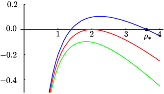
Figure 10: Graph of the r.h.s. of (41) for $\alpha\equiv\gamma r_{0}^{2}/2\sigma t_{0}=0.2,0.25,0.3$. When $\alpha<1/4$ Eq. (41) has a fixed point $\rho=\rho_{\ast}>r_{c}$, which grows indefinitely with time, so that all domains grow and the total domain area grows to infinity. When $\alpha>1/4$ all domains shrink to zero. The correct asymptotic behavior is found by selecting the separatrix between these two extreme cases.

References

- [1] M. Abramowitz and I. Stegun. Handbook of mathematical functions : with formulas, graph, and mathematical tables. Dover, 1965.
- [2] B. Alberts, A. Johnson, J. Lewis, M. Raff, K. Roberts, and P. Walter. Molecular Biology of the Cell. Garland Science, 2007.
- [3] U. Alon, M.G. Surette, N. Barkai, and S. Leibler. Robustness in bacterial chemotaxis. Nature, 397:168–171, 1999.
- [4] S.J. Altschuler, S.B. Angenent, Y. Wang, and L.F. Wu. On the spontaneous emergence of cell polarity. Nature, 454:886–890, 2008.
- [5] H.C. Berg and E.M. Purcell. Physics of chemoreception. Biophys. J., 20:193–219, 1977.
- [6] C. Beta, G. Amselem, and E. Bodenschatz. A bistable mechanism for directional sensing. New J. of Phys., 2008.
- [7] A.J. Bray. Theory of phase ordering kinetics. Adv. Phys., 43:357–459, 1994.
- [8] A. Ciliberto, F. Capuani, and J. J. Tyson. Modeling networks of coupled enzymatic reactions using the total quasi-steady state approximation. PLoS Comput Biol, 3:e45, 2007.
- [9] A. de Candia, A. Gamba, F. Cavalli, A. Coniglio, S. Di Talia, F. Bussolino, and G. Serini. A simulation environment for directional sensing as a phase separation process. Sci. STKE, 378:pl1, 2007.
- [10] T. Ferraro, A. de Candia, A. Gamba, and A. Coniglio. Spatial signal amplification in cell biology: a lattice-gas model for self-tuned phase ordering. Europh. Lett., 83:50009–1–5, 2008.
- [11] A. Gamba, A. de Candia, S. Di Talia, A. Coniglio, F. Bussolino, and G. Serini. Diffusion limited phase separation in eukaryotic chemotaxis. Proc. Nat. Acad. Sci. U.S.A., 102:16927–16932, 2005.
- [12] A. Gamba, I. Kolokolov, V. Lebedev, and G. Ortenzi. Patch coalescence as a mechanism for eukaryotic directional sensing. Phys. Rev. Lett., 99:158101–1–4, 2007.
- [13] C.W. Gardiner. Handbook of stochastic methods for physics, chemistry and the natural sciences. Springer, New York, 1983.
- [14] A. Gierer and H. Meinhardt. A theory of biological pattern formation. Kybernetik, 12:30–39, 1972.
- [15] P.C. Hohenberg and B.I. Halperin. Theory of dynamic critical phenomena. Rev. Mod. Phys., 49:436–479, 1977.
- [16] P.A. Iglesias and P.N. Devreotes. Navigating through models of chemotaxis. Curr. Op. Cell Biol., 20:1–6, 2007.
- [17] L.D. Landau and E.M. Lifshitz. Statistical Physics (Part I), volume 5 of Course of Theoretical Physics. Pergamon Press, third edition, 1980.
- [18] D. A. Lauffenburger and A. F. Horwitz. Cell migration: a physically integrated molecular process. Cell, 84:359–369, 1996.
- [19] E.M. Lifshitz and L.P. Pitaevskii. Physical Kinetics, volume 10 of Course of Theoretical Physics. Pergamon Press, first edition, 1981.
- [20] E. Marco, R. Wedlich-Soldner, R. Li, S. J. Altschuler, and L. F. Wu. Endocytosis optimizes the dynamic localization of membrane proteins that regulate cortical polarity. Cell, 129:411–22, 2007.
- [21] M. Meier-Schellersheim, X. Xu, B. Angermann, E.J. Kunkel, T. Jin, and R.N. Germain. Key role of local regulation in chemosensing revealed by a new molecular interaction-based modeling method. Plos Comp. Biol., 2:710–24, 2006.
- [22] Y. Mori, A. Jilkine, and L. Edelstein-Keshet. Wave-pinning and cell polarity from a bistable reaction-diffusion system. Biophys J, 2008.
- [23] C. Parent. Making all the right moves: chemotaxis in neutrophils and Dictyostelium. Curr. Opin. Cell Biol., 16:4–13, 2004.
- [24] C.A. Parent and P.N. Devreotes. A cell’s sense of direction. Science, 284:765–769, 1999.
- [25] M. Postma, J. Roelofs, J. Goedhart, H.M. Loovers, A.J. Visser, and P.J. Van Haastert. Sensitization of Dictyostelium chemotaxis by phosphoinositide-3-kinase-mediated self-organizing signalling patches. J. Cell Sci., 117:2925–35, 2004.
- [26] A.J. Ridley, M.A. Schwartz, K. Burridge, R.A. Firtel, M.H. Ginsberg, G. Borisy, J.T. Parsons, and A.R. Horwitz. Cell migration: integrating signals from front to back. Science, 302:1704–9, 2003.
- [27] C. Sachs, M. Hildebrand, S. Völkening, J. Wintterlin, and G. Ertl. Self-organization in a surface reaction: from the atomic to the mesoscopic scale. Science, 293:1635–1638, 2001.
- [28] A. Samadani, J. Mettetal, and A. van Oudenaarden. Cellular asymmetry and individuality in directional sensing. Proc. Nat. Acad. U.S.A., 103:11549–11554, 2006.
- [29] F. Schlögl. Z. Phys., 253:147, 1972.
- [30] E. Schöll. Stochastic Processes in Physics, Chemistry, and Biology, volume 557 of Lecture Notes in Physics, pages 437–451. Springer, 2000.
- [31] C. Sire and S.N. Majumdar. Coarsening in the q-state Potts model and the Ising model with globally conserved magnetization. Phys. Rev. E, 52:244, 1995.
- [32] R. Skupsky, W. Losert, and R. J. Nossal. Distinguishing modes of eukaryotic gradient sensing. Biophys. J., 89(4):2806–23, 2005.
- [33] L. Song, S. M. Nadkarni, H. U. Bodeker, C. Beta, A. Bae, C. Franck, W. J. Rappel, W. F. Loomis, and E. Bodenschatz. Dictyostelium discoideum chemotaxis: threshold for directed motion. Eur. J. Cell Biol., 85:981–9, 2006.
- [34] Z. Tong, X. D. Gao, A. S. Howell, I. Bose, D. J. Lew, and E. Bi. Adjacent positioning of cellular structures enabled by a Cdc42 GTPase-activating protein-mediated zone of inhibition. J. Cell Biol., 179:1375–84, 2007.
- [35] P. J. van Haastert, I. Keizer-Gunnink, and A. Kortholt. Essential role of PI3-kinase and phospholipase A2 in Dictyostelium discoideum chemotaxis. J. Cell Biol., 177:809–16, 2007.
- [36] N.G. van Kampen. Stochastic Processes in Physics and Chemistry. North-Holland, third edition, 2007.
- [37] R. Wedlich-Soldner, S. Altschuler, L. Wu, and R. Li. Spontaneous cell polarization through actomyosin-based delivery of the Cdc42 GTPase. Science, 299:1231–5, 2003.
- [38] R. Wedlich-Soldner and R. Li. Spontaneous cell polarization: undermining determinism. Nat. Cell Biol., 5:267–70, 2003.
- [39] R. Wedlich-Soldner, S.C. Wai, T. Schmidt, and R. Li. Robust cell polarity is a dynamic state established by coupling transport and GTPase signaling. J. Cell Biol., 166:889–900, 2004.
- [40] S. Wehner, P. Hoffmann, D. Schmeißer, H.R. Brand, and J. Kuppers. Spatiotemporal patterns of external noise-induced transitions in a bistable reaction-diffusion system: photoelectron emission microscopy experiments and modeling. Phys. Rev. Lett., 95:038301–1–4, 2005.