The rigorous solution for the average distance of a Sierpinski network

Abstract

The closed-form solution for the average distance of a deterministic network–Sierpinski network–is found. This important quantity is calculated exactly with the help of recursion relations, which are based on the self-similar network structure and enable one to derive the precise formula analytically. The obtained rigorous solution confirms our previous numerical result, which shows that the average distance grows logarithmically with the number of network nodes. The result is at variance with that derived from random networks.

I Introduction

Structural properties CoRoTrVi07 , such as degree distribution BaAl99 , average distance WaSt98 , degree correlations Newman02 , community GiNe02 , motifs MiShItKaChAl02 , fractality SoHaMa05 , and symmetry XiXiWaWa08 , have received much attention in the field of complex networks, since these features play significant roles in characterizing and understanding complex networked systems in nature and society. Among these important features, average distance characterizes the small-world behavior commonly observed in various disparate real networks WaSt98 . It has been established that average distance is related to other structural properties, such as degree distribution ChLu02 ; CoHa03 , fractality SoHaMa06 ; ZhZhZo07 and symmetry XiMaiWaXiWa08 . On the other hand, average distance has an important consequence on dynamical processes taking placing on networks, including disease spreading WaSt98 , routing YaZhHuFuWa06 ; ZhCoFeRaRoZh08 , robustness SoHaMa06 ; ZhZhZo07 , percolation ZhZhZoCh08 , and so on. Thus far, average distance has become a focus of attention for the scientific community DoMeSa03 ; FrFrHo04 ; Lolo03 ; HoSiFrFrSu05 ; DoMeOl06 ; ZhZhChYiGu08 .

Using above-mentioned structural properties, extensive empirical studies on diverse real systems have been done with an attempt to uncover and understand the generic features and complexity of these systems, and various network models have been proposed to reproduce or explaining the common characteristics of real-life networks AlBa02 ; DoMe02 ; Ne03 ; BoLaMoChHw06 . Recently, inspired by the well-known Sierpinski gasket, we proposed a novel network, called Sierpinski network ZhZhFaGuZh07 . The Sierpinski network belongs to a deterministically growing class of networks that have attracted considerable attention and have turned out to be a useful tool BaRaVi01 ; DoGoMe02 ; JuKiKa02 ; RaSoMoOlBa02 ; AnHeAnSi05 ; Hi07 ; BoGoGu08 . Many relevant topological properties of Sierpinski network such as degree distribution, clustering coefficient, and strength distribution have been determined analytically ZhZhFaGuZh07 . Also, the average distance of Sierpinski network has been been investigated numerically, which was shown to behaves a logarithmic scaling with the number of network nodes (vertices) ZhZhFaGuZh07 .

In view of the importance and usefulness of the quantity—average distance, here we derive a closed-form formula for the average distance characterizing the Sierpinski network. The analytic method is on the basis of the recursive construction and self-similar structure of Sierpinski network. Our precise result shows that the average distance of Sierpinski network increases logarithmically with the number of nodes. This scaling behaves differently from that of random networks ChLu02 ; CoHa03 . Our rigorous solution confirms the scaling between average distance and number of network nodes that was previously obtained numerically in ZhZhFaGuZh07 .

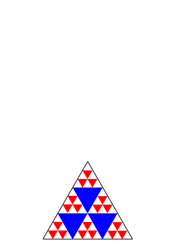
Figure 1: The first two stages in the construction for a variant of Sierpinkski gasket.

II Brief introduction to the Sierpinski network

The Sierpinski network is derived from a variation of the Sierpinski gasket Si15 . The Sierpinski gasket variant, shown in figure 1, is constructed as follows Ha92 . We start with an equilateral triangle, and we denote this initial configuration by generation $t=0$. Then in the first generation $t=1$, we divide the three sides of the equilateral triangle in three, then join these points and remove the three down pointing triangles. This forms six copies of the original triangle, and the procedure is repeated indefinitely for all the new copies. In the limit of infinite $t$ generations, we get a fractal variant of the Sierpinski gasket. The Hausdorff dimension of the obtained fractal is $d_{f}=1+\ln 2/\ln 3$ Hu81 . From the fractal, one can define the Sierpinski network ZhZhFaGuZh07 , where vertices correspond to the removed triangles and two vertices are connected if the boundaries of the corresponding triangles contact each other. Note that for uniformity, the three sides of the initial equilateral triangle at step 0 also correspond to three different vertices. Figure 2 shows the network construction process.

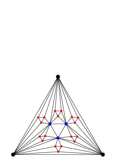
Figure 2: Illustration of the network corresponding to the fractal shown in figure 1.

The Sierpinski network can be generated using an iterative algorithm ZhZhFaGuZh07 . We denote the network after $t$ iterations by $F_{t}$ with $t\geq 0$. Then the network is constructed as follows: For $t=0$, $F_{t}$ is a triangle. Next, three nodes are added into the original triangle. These three new nodes are connected to each other forming a new triangle, and both ends of each edge of the new triangle are linked to a node of the original triangle. Thus $F_{1}$ is obtained, see figure 3. For $t\geq 1$, we can get $F_{t}$ from $F_{t-1}$. For each of the existing triangles of $F_{t-1}$ that does not consist of three simultaneously emerging nodes and has never generated a node before, we define it an active triangle. We replace each of the active triangles in $F_{t-1}$ by the connected cluster on the right hand of figure 3 to obtain $F_{t}$.

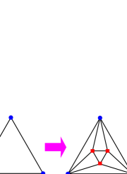
Figure 3: Iterative construction method for the network.

The resulting network presents the typical characteristics of real-life networks in nature and society ZhZhFaGuZh07 . It has power-law distributions of degree and strength, with exponents $\gamma_{k}=2+\frac{\ln 2}{\ln 3}$ and $\gamma_{s}=\frac{3}{2}+\frac{\ln 2}{2\ln 3}$, respectively. There also exists a power-law scaling relation between the strength $s$ and degree $k$ of an individual node, i.e. $s\sim k^{2}$. On the other hand, for any individual vertex, its clustering coefficient is $C(k)=\frac{4}{k}-\frac{1}{k-1}$; so when $k$ is large, $C(k)$ is approximately inversely proportional to degree $k$. The mean value $C$ of clustering coefficients of all vertices is very large, which asymptotically reaches a constant value 0.598. Moreover, the network is a maximal planar graph.

III Rigorous derivation of average distance

After introducing the Sierpinski network, we now derive analytically the average distance. We represent all the shortest path lengths of network $F_{t}$ as a matrix in which the entry $d_{ij}$ is the distance between node $i$ and $j$ that is the length of a shortest path joining $i$ and $j$. A measure of the typical separation between two nodes in $F_{t}$ is given by the average distance $d_{t}$ defined as the mean of distances over all pairs of nodes:

$$d_{t}=\frac{D_{t}}{N_{t}(N_{t}-1)/2}\,,$$ (1)

where

$$D_{t}=\sum_{i\in F_{t},\,j\in F_{t},\,i\neq j}d_{ij}$$ (2)

denotes the sum of the distances between two nodes over all couples.

Figure 4: Schematic illustration of second construction means of Sierpinski network. $F_{t+1}$ may be obtained by joining six copies of $F_{t}$ denoted as $F_{t}^{(\eta)}$ $(\eta=1,\cdots,6)$, which are connected to one another at the edge nodes.

III.1 Recursive equation for total distances

We continue by exhibiting the procedure of determining the total distance and present the recurrence formula, which allows us to obtain $D_{t+1}$ of the $t+1$ generation from $D_{t}$ of the $t$ generation. The Sierpinski network $F_{t}$ has a self-similar structure that allows one to calculate $D_{t}$ analytically HiBe06 . As shown in figure 4, network $F_{t+1}$ may be obtained by joining at six edge nodes (i.e., $A$, $B$, $C$, $X$, $Y$, and $Z$) six copies of $F_{t}$ that are labeled as $F_{t}^{(1)}$, $\cdots$, $F_{t}^{(6)}$ Bobe05 . From this we can obtain the recursion relation

$$N_{t+1}=6\,N_{t}-12,$$ (3)

for the network order $N_{t}$, which is the number of nodes in the graph of generation $t$. This recursion, coupled with $N_{0}=3$, yields

$$N_{t}=\frac{3\times 6^{t}+12}{5}$$ (4)

as previously obtained in ZhZhFaGuZh07 .

According to the second construction method, the total distance $D_{t+1}$ satisfies the recursion relation

$$D_{t+1}=6\,D_{t}+\Delta_{t}-6,$$ (5)

where $\Delta_{t}$ is the sum over all shortest path length whose endpoints are not in the same $F_{t}^{(\eta)}$ branch. The last term -6 on the right-hand side of Eq. (5) compensates for the overcounting of certain paths: the shortest path between $A$ and $X$, with length 1, is included in both $F_{t}^{(1)}$ and $F_{t}^{(2)}$. Similarly the shortest path between $A$ and $Y$, the shortest path between $B$ and $X$, the shortest path between $B$ and $Z$, the shortest path between $C$ and $Y$, and the shortest path between $C$ and $Z$, are all computed twice. To determine $D_{t}$, all that is left is to calculate $\Delta_{t}$.

III.2 Definition of crossing distance

In order to compute $\Delta_{t}$, we classify the nodes in $F_{t+1}$ into two categories: the six edge nodes (such as $A$, $B$, $C$, $X$, $Y$, and $Z$ in figure 4) are called hub nodes, while the other nodes are named non-hub nodes. Thus $\Delta_{t}$, named the crossing distance, can be obtained by summing the following path length that are not included in the distance of node pairs in $F_{t}^{(\eta)}$: length of the shortest paths between non-hub and non-hub nodes, length of the shortest paths between hub and non-hub nodes, and length of the shortest paths between hub nodes (i.e., $d_{AZ}$, $d_{BY}$, and $d_{CZ}$).

Denote $\Delta_{t}^{\alpha,\beta}$ as the sum of all shortest paths between non-hub nodes, whose endpoints are in $F_{t}^{(\alpha)}$ and $F_{t}^{(\beta)}$, respectively. That is to say, $\Delta_{t}^{\alpha,\beta}$ rules out the paths with endpoint at the hub nodes belonging to $F_{t}^{(\alpha)}$ or $F_{t}^{(\beta)}$. For example, each path contributed to $\Delta_{t}^{1,2}$ does not end at node $A$, $B$, $X$ or $Y$. On the other hand, let $\Omega_{t}^{\eta}$ be the set of non-hub nodes in $F_{t}^{(\eta)}$. Then the total sum $\Delta_{t}$ is given by

$$\Delta_{t}=\Delta_{t}^{1,2} + \Delta_{t}^{1,3}+\Delta_{t}^{1,4}+\Delta_{t}^{1,5}+\Delta_{t}^{1,6}+\Delta_{t}^{2,3}+\Delta_{t}^{2,4}+\Delta_{t}^{2,5}+\Delta_{t}^{2,6}+\Delta_{t}^{3,4}+\Delta_{t}^{3,5}+\Delta_{t}^{3,6}+\Delta_{t}^{4,5}$$ (6)

$$+ \Delta_{t}^{4,6}+\Delta_{t}^{5,6}+\sum_{j\in\Omega_{t}^{4}}d_{Aj}+\sum_{j\in\Omega_{t}^{5}}d_{Aj}+\sum_{j\in\Omega_{t}^{6}}d_{Aj}+\sum_{j\in\Omega_{t}^{2}}d_{Bj}+\sum_{j\in\Omega_{t}^{3}}d_{Bj}+\sum_{j\in\Omega_{t}^{4}}d_{Bj}$$

$$+ \sum_{j\in\Omega_{t}^{1}}d_{Cj}+\sum_{j\in\Omega_{t}^{2}}d_{Cj}+\sum_{j\in\Omega_{t}^{6}}d_{Cj}+\sum_{j\in\Omega_{t}^{3}}d_{Xj}+\sum_{j\in\Omega_{t}^{4}}d_{Xj}+\sum_{j\in\Omega_{t}^{5}}d_{Xj}+\sum_{j\in\Omega_{t}^{1}}d_{Yj}+\sum_{j\in\Omega_{t}^{5}}d_{Yj}$$

$$+ \sum_{j\in\Omega_{t}^{6}}d_{Yj}+\sum_{j\in\Omega_{t}^{1}}d_{Zj}+\sum_{j\in\Omega_{t}^{2}}d_{Zj}+\sum_{j\in\Omega_{t}^{3}}d_{Zj}+d_{AZ}+d_{BY}+d_{CX}$$

By symmetry, $\Delta_{t}^{1,2}=\Delta_{t}^{1,6}=\Delta_{t}^{2,3}+\Delta_{t}^{3,4}=\Delta_{t}^{4,5}=\Delta_{t}^{5,6}$, $\Delta_{t}^{1,3}=\Delta_{t}^{1,5}=\Delta_{t}^{2,4}=\Delta_{t}^{2,6}=\Delta_{t}^{3,5}=\Delta_{t}^{4,6}$, $\Delta_{t}^{1,4}=\Delta_{t}^{2,5}=\Delta_{t}^{3,6}$, $\sum_{j\in\Omega_{t}^{4}}d_{Aj}=\sum_{j\in\Omega_{t}^{5}}d_{Aj}=\sum_{j\in\Omega_{t}^{6}}d_{Aj}=\sum_{j\in\Omega_{t}^{2}}d_{Bj}=\sum_{j\in\Omega_{t}^{3}}d_{Bj}=\sum_{j\in\Omega_{t}^{4}}d_{Bj}=\sum_{j\in\Omega_{t}^{1}}d_{Cj}=\sum_{j\in\Omega_{t}^{2}}d_{Cj}=\sum_{j\in\Omega_{t}^{6}}d_{Cj}=\sum_{j\in\Omega_{t}^{3}}d_{Xj}=\sum_{j\in\Omega_{t}^{4}}d_{Xj}=\sum_{j\in\Omega_{t}^{5}}d_{Xj}=\sum_{j\in\Omega_{t}^{1}}d_{Yj}=\sum_{j\in\Omega_{t}^{5}}d_{Yj}=\sum_{j\in\Omega_{t}^{6}}d_{Yj}=\sum_{j\in\Omega_{t}^{1}}d_{Zj}=\sum_{j\in\Omega_{t}^{2}}d_{Zj}=\sum_{j\in\Omega_{t}^{3}}d_{Zj}$, and $d_{AZ}=d_{BY}=d_{CX}=2$, so Eq. (6) can be simplified as

$$\Delta_{t}=6\,\Delta_{t}^{1,2}+6\,\Delta_{t}^{1,3}+3\,\Delta_{t}^{1,4}+18\,\sum_{j\in\Omega_{t}^{4}}d_{Aj}+6.$$ (7)

Having $\Delta_{t}$ in terms of the quantities of $\Delta_{t}^{1,2}$, $\Delta_{t}^{1,3}$, $\Delta_{t}^{1,4}$, and $\sum_{j\in\Omega_{t}^{4}}d_{Aj}$, the next step is to explicitly determine these quantities.

Figure 5: Illustration of the classification of interior nodes in $F_{t}^{(\eta)}$ $(\eta=1,\cdots,6)$, from which we can derive recursively the classification of interior nodes in network $F_{t+1}$.

III.3 Classification of interior nodes

To calculate the crossing distance $\Delta_{t}^{1,2}$, $\Delta_{t}^{1,3}$, $\Delta_{t}^{1,4}$, and $\sum_{j\in\Omega_{t}^{4}}d_{Aj}$, we classify interior nodes in network $F_{t+1}$ into seven different parts according to their shortest path lengths to each of the three hub nodes (i.e. $A$, $B$, $C$) of the peripheral triangle $\triangle ABC$. Notice that nodes $A$, $B$, $C$ themselves are not partitioned into any of the seven parts represented as $P_{1}$, $P_{2}$, $P_{3}$, $P_{4}$, $P_{5}$, $P_{6}$, and $P_{7}$, respectively. The classification of nodes is shown in figure 5. For any interior node $v$, we denote the shortest path lengths from $v$ to $A$, $B$, $C$ as $a$, $b$, and $c$, respectively. By construction, $a$, $b$, $c$ can differ by at most $1$ since vertices $A$, $B$, $C$ are adjacent. Then the classification function $class(v)$ of node $v$ is defined to be

$$class(v)=\left\{\begin{array}[]{lc}{\displaystyle{P_{1}}}&\quad\hbox{for}\ a<b=c,\\ {\displaystyle{P_{2}}}&\quad\hbox{for}\ b<a=c,\\ {\displaystyle{P_{3}}}&\quad\hbox{for}\ c<a=b,\\ {\displaystyle{P_{4}}}&\quad\hbox{for}\ a=c<b,\\ {\displaystyle{P_{5}}}&\quad\hbox{for}\ a=b<c,\\ {\displaystyle{P_{6}}}&\quad\hbox{for}\ b=c<a,\\ {\displaystyle{P_{7}}}&\quad\hbox{for}\ a=b=c.\\ \end{array}\right.$$ (8)

It should be mentioned that the definition of node classification is recursive. For instance, class $P_{1}$ and $P_{4}$ in $F_{t}^{(1)}$ belong to class $P_{1}$ in $F_{t+1}$, class $P_{3}$ and $P_{5}$ in $F_{t}^{(1)}$ belong to class $P_{2}$ in $F_{t+1}$, class $P_{2}$, $P_{6}$, and $P_{7}$ in $F_{t}^{(1)}$ belong to class $P_{5}$ in $F_{t+1}$. Since the three nodes $A$, $B$, and $C$ are symmetrical, in the Sierpinski network we have the following equivalent relations from the viewpoint of class cardinality: classes $P_{1}$, $P_{2}$, and $P_{3}$ are equivalent to one another, and it is the same with classes $P_{4}$, $P_{5}$, and $P_{6}$. We denote the number of nodes in network $F_{t}$ that belong to class $P_{1}$ as $N_{t,P_{1}}$, the number of nodes in class $P_{2}$ as $N_{t,P_{2}}$, and so on. By symmetry, we have $N_{t,P_{1}}=N_{t,P_{2}}=N_{t,P_{3}}$ and $N_{t,P_{4}}=N_{t,P_{5}}=N_{t,P_{6}}$. Therefore in the following computation we will only consider $N_{t,P_{1}}$, $N_{t,P_{4}}$, and $N_{t,P_{7}}$. It is easy to conclude that

$$N_{t} =N_{t,P_{1}}+N_{t,P_{2}}+N_{t,P_{3}}+N_{t,P_{4}}+N_{t,P_{5}}+N_{t,P_{6}}+N_{t,P_{7}}+3$$

$$=3\,N_{t,P_{1}}+3\,N_{t,P_{4}}+N_{t,P_{7}}+3.$$ (9)

Considering the self-similar structure of Sierpinski network, we can easily know that at time $t+1$, the quantities $N_{t+1,P_{1}}$, $N_{t+1,P_{4}}$, and $N_{t+1,P_{7}}$ evolve according to the following recursive equations

$$\left\{\begin{array}[]{ccc}N_{t+1,P_{1}}&=&3\,N_{t,P_{1}}+4\,N_{t,P_{4}}+N_{t,P_{7}}\,,\\ N_{t+1,P_{4}}&=&3\,N_{t,P_{1}}+N_{t,P_{4}}+N_{t,P_{7}}+1\,,\\ N_{t+1,P_{7}}&=&3\,N_{t,P_{4}}\,,\\ \end{array}\right.$$ (13)

where we have used the equivalent relations $N_{t,P_{1}}=N_{t,P_{2}}=N_{t,P_{3}}$ and $N_{t,P_{4}}=N_{t,P_{5}}=N_{t,P_{6}}$. With the initial condition $N_{2,P_{1}}=4$, $N_{2,P_{4}}=2$, and $N_{2,P_{7}}=3$, we can solve the recursive equation (13) to obtain

$$\left\{\begin{array}[]{ccc}N_{t,P_{1}}&=&\frac{1}{240}\left[-112+25\times(-2)^{t}+27\times 6^{t}\right]\,,\\ N_{t,P_{4}}&=&\frac{1}{120}\left[16-25\times(-2)^{t}+9\times 6^{t}\right]\,,\\ N_{t,P_{7}}&=&=\frac{1}{80}\left[32+25\times(-2)^{t}+3\times 6^{t}\right]\,.\\ \end{array}\right.$$ (17)

For a node $v$ in network $F_{t+1}$, we are also interested in the smallest value of the shortest path length from $v$ to any of the three peripheral hub nodes $A$, $B$, and $C$. We denote the shortest distance as $f_{v}$, which can be defined to be

$$f_{v}=min(a,b,c).$$ (18)

Let $d_{t,P_{1}}$ denote the sum of $f_{v}$ of all nodes belonging to class $P_{1}$ in network $F_{t}$. Analogously, we can also define the quantities $d_{t,P_{2}}$, $d_{t,P_{3}}$, $\cdots$, $d_{t,P_{7}}$. Again by symmetry, we have $d_{t,P_{1}}=d_{t,P_{2}}=d_{t,P_{3}}$, $d_{t,P_{4}}=d_{t,P_{5}}=d_{t,P_{6}}$, and $d_{t,P_{1}}$, $d_{t,P_{4}}$, $d_{t,P_{7}}$ can be written recursively as follows:

$$\left\{\begin{array}[]{ccc}d_{t+1,P_{1}}&=&3\,d_{t,P_{1}}+4\,d_{t,P_{4}}+d_{t,P_{7}}\,,\\ d_{t+1,P_{4}}&=&3\,d_{t,P_{1}}+d_{t,P_{4}}+d_{t,P_{7}}+3\,N_{t,P_{1}}+1\,,\\ d_{t+1,P_{7}}&=&3\,(d_{t,P_{4}}+N_{t,P_{4}})\,.\\ \end{array}\right.$$ (22)

Substituting Eq. (17) into Eq. (22), and considering the initial condition $d_{2,P_{1}}=4$, $d_{2,P_{4}}=2$, and $d_{2,P_{7}}=6$, Eq. (22) is solved inductively

$$\left\{\begin{array}[]{ccc}d_{t,P_{1}}&=&\frac{1}{25600}[2048+327\times 6^{t}+990t\times 6^{t}+25(33+70t)2^{t}e^{i\pi t}]\,,\\ d_{t,P_{4}}&=&\frac{1}{12800}\left[-2075(-2)^{t}-1024(-1)^{2t}+699\times 6^{t}+10t\left(-175\times(-2)^{t}+33\times 6^{t}\right)\right]\,,\\ d_{t,P_{7}}&=&\frac{1}{25600}[4096+1329\times 6^{t}+330t\times 6^{t}+25(359+210t)2^{t}\,e^{i\pi t}]\,.\end{array}\right.$$ (26)

III.4 Calculation of crossing distances

Having obtained the quantities $N_{t,P_{i}}$ and $d_{t,P_{i}}$ ($i=1,2,\cdots,7$), we now begin to determine the crossing distance $\Delta_{t}^{1,2}$, $\Delta_{t}^{1,3}$, $\Delta_{t}^{1,4}$, and $\sum_{j\in\Omega_{t}^{4}}d_{Aj}$ expressed as a function of $N_{t,P_{i}}$ and $d_{t,P_{i}}$. Here we only give the computation details of $\Delta_{t}^{1,2}$, while the computing processes of $\Delta_{t}^{1,3}$, $\Delta_{t}^{1,4}$, and $\sum_{j\in\Omega_{t}^{4}}d_{Aj}$ are similar. For convenience of computation, we use $\Gamma_{t}^{\eta,i}$ to denote the set of interior nodes belonging to class $P_{i}$ in $F_{t}^{(\eta)}$. Then $\Delta_{t}^{1,2}$ can be written as

$$\Delta_{t}^{1,2}=\sum_{\begin{subarray}{c}u\in\Gamma_{t}^{1,1},\,\,v\in F_{t}^{(2)}\\ v\neq A,X,Y\end{subarray}}d_{uv} + \sum_{\begin{subarray}{c}u\in\Gamma_{t}^{1,2},\,\,v\in F_{t}^{(2)}\\ v\neq A,X,Y\end{subarray}}d_{uv}+\sum_{\begin{subarray}{c}u\in\Gamma_{t}^{1,3},\,\,v\in F_{t}^{(2)}\\ v\neq A,X,Y\end{subarray}}d_{uv}+\sum_{\begin{subarray}{c}u\in\Gamma_{t}^{1,4},\,\,v\in F_{t}^{(2)}\\ v\neq A,X,Y\end{subarray}}d_{uv}$$ (27)

$$+ \sum_{\begin{subarray}{c}u\in\Gamma_{t}^{1,5},\,\,v\in F_{t}^{(2)}\\ v\neq A,X,Y\end{subarray}}d_{uv}+\sum_{\begin{subarray}{c}u\in\Gamma_{t}^{1,6},\,\,v\in F_{t}^{(2)}\\ v\neq A,X,Y\end{subarray}}d_{uv}+\sum_{\begin{subarray}{c}u\in\Gamma_{t}^{1,7},\,\,v\in F_{t}^{(2)}\\ v\neq A,X,Y\end{subarray}}d_{uv}.$$

The seven terms on the right-hand side of Eq. (27) are represented consecutively as $\delta_{t}^{i}$ ($i=1,2,\cdots,7$). Next we will calculate the quantities $\delta_{t}^{i}$. By symmetry, $\delta_{t}^{1}=\delta_{t}^{2}$, $\delta_{t}^{5}=\delta_{t}^{6}$. Therefore, we need only to compute $\delta_{t}^{1}$, $\delta_{t}^{3}$, $\delta_{t}^{4}$, $\delta_{t}^{5}$ and $\delta_{t}^{7}$. Firstly, we evaluate $\delta_{t}^{1}$. By definition,

$$\delta_{t}^{1} = \sum_{\begin{subarray}{c}u\in\Gamma_{t}^{1,1},\,\,v\in F_{t}^{(2)}\\ v\neq A,X,Y\end{subarray}}d_{uv}$$ (28)

$$= \sum_{u\in\Gamma_{t}^{1,1},\,v\in\Gamma_{t}^{2,1}\bigcup\Gamma_{t}^{2,4}\bigcup\Gamma_{t}^{2,6}\bigcup\Gamma_{t}^{2,7}}(d_{uA}+d_{Av})+\sum_{u\in\Gamma_{t}^{1,1},\,v\in\Gamma_{t}^{2,3}}(d_{uA}+d_{AY}+d_{Yv})$$

$$+\sum_{u\in\Gamma_{t}^{1,1},\,v\in\Gamma_{t}^{2,2}\bigcup\Gamma_{t}^{2,5}}(d_{uA}+d_{AX}+d_{Xv})$$

$$= N_{t,P_{1}}(3d_{t,P_{1}}+3d_{t,P_{4}}+d_{t,P_{7}}+2N_{t,P_{1}}+N_{t,P_{4}})+d_{t,P_{1}}(3N_{t,P_{1}}+3N_{t,P_{4}}+N_{t,P_{7}}).$$

Proceeding similarly, we obtain

$$\delta_{t}^{3}=N_{t,P_{1}}(3d_{t,P_{1}}+3d_{t,P_{4}}+d_{t,P_{7}}+4N_{t,P_{1}}+3N_{t,P_{4}}+N_{t,P_{7}})+d_{t,P_{1}}(3N_{t,P_{1}}+3N_{t,P_{4}}+N_{t,P_{7}}),$$ (29)

$$\delta_{t}^{4}=N_{t,P_{2}}(3d_{t,P_{1}}+3d_{t,P_{4}}+d_{t,P_{7}}+N_{t,P_{1}})+d_{t,P_{2}}(3N_{t,P_{1}}+3N_{t,P_{4}}+N_{t,P_{7}}),$$ (30)

$$\delta_{t}^{5}=N_{t,P_{2}}(3d_{t,P_{1}}+3d_{t,P_{4}}+d_{t,P_{7}}+2N_{t,P_{1}}+N_{t,P_{4}})+d_{t,P_{2}}(3N_{t,P_{1}}+3N_{t,P_{4}}+N_{t,P_{7}}),$$ (31)

and

$$\delta_{t}^{7}=N_{t,P_{3}}(3d_{t,P_{1}}+3d_{t,P_{4}}+d_{t,P_{7}}+N_{t,P_{1}})+d_{t,P_{7}}(3N_{t,P_{1}}+3N_{t,P_{4}}+N_{t,P_{7}}).$$ (32)

With the obtained results for $\delta_{t}^{i}$, we have

$$\Delta_{t}^{1,2} = 2(3d_{t,P_{1}}+3d_{t,P_{4}}+d_{t,P_{7}})(3N_{t,P_{1}}+3N_{t,P_{4}}+N_{t,P_{7}})+N_{t,P_{1}}(3N_{t,P_{1}}+3N_{t,P_{4}}+N_{t,P_{7}})$$ (33)

$$+2(N_{t,P_{1}}+N_{t,P_{4}})(2N_{t,P_{1}}+N_{t,P_{4}})+N_{t,P_{1}}(N_{t,P_{4}}+N_{t,P_{7}})+(N_{t,P_{1}})^{2}.$$

Analogously, we find

$$\Delta_{t}^{1,3} = 2(3d_{t,P_{1}}+3d_{t,P_{4}}+d_{t,P_{7}})(3N_{t,P_{1}}+3N_{t,P_{4}}+N_{t,P_{7}})+2(N_{t,P_{1}})^{2}+2N_{t,P_{1}}(3N_{t,P_{1}}+3N_{t,P_{4}}+N_{t,P_{7}})$$ (34)

$$+N_{t,P_{4}}(3N_{t,P_{1}}+3N_{t,P_{4}}+N_{t,P_{7}})+(N_{t,P_{1}}+2N_{t,P_{4}}+N_{t,P_{7}})(2N_{t,P_{1}}+N_{t,P_{4}}),$$

$$\Delta_{t}^{1,4}=2(3d_{t,P_{1}}+3d_{t,P_{4}}+d_{t,P_{7}})(3N_{t,P_{1}}+3N_{t,P_{4}}+N_{t,P_{7}})+(3N_{t,P_{1}}+3N_{t,P_{4}}+N_{t,P_{7}})^{2}+3(N_{t,P_{1}})^{2},$$ (35)

and

$$\sum_{j\in\Omega_{t}^{4}}d_{Aj}=(3d_{t,P_{1}}+3d_{t,P_{4}}+d_{t,P_{7}})+(3N_{t,P_{1}}+3N_{t,P_{4}}+N_{t,P_{7}})+N_{t,P_{1}}.$$ (36)

Substituting Eqs. (33), (34), (35), and (36) into Eq. (7), we the final expression for cross distances $\Delta_{t}$,

$$\Delta_{t}=\frac{1}{19200}\big{[} - 17920+95040\times 6^{t}+160380\times 6^{2t}+50\times 2^{t}(-32+27\times 6^{t})e^{i\pi t}+44550t\times 6^{2t}$$ (37)

$$+ e^{2i\pi t}(6875\times 4^{t}-82944\times 6^{t}+8019\times 6^{2t}+26730t\times 6^{2t})\big{]}.$$

III.5 Rigorous result of average distance

With the above-obtained results and recursion relations, we now readily calculate the sum of the shortest path lengths between all pairs of nodes. Inserting Eq. (37) into Eq. (5) and using the initial condition $D_{2}=555$, Eq. (5) is solved inductively,

$$D_{t}=\frac{1}{192000}\Big{[}266240-34375\times 4^{t} + 2000\times(-2)^{t}+225264\times 6^{t}-750(-12)^{t}$$ (38)

$$+ 27621\times 6^{2t}+20160t\times 6^{t}+23760t\times 6^{2t}\Big{]}.$$

Substituting Eq. (38) into Eq. (1) yields the exactly analytic expression for average distance

$$d_{t}=\frac{1}{34560(84+57\times 6^{t}+9\times 6^{2t})} \Big{[}266240-34375\times 4^{t}+2000\times(-2)^{t}+225264\times 6^{t}$$ (39)

$$- 750(-12)^{t}+27621\times 6^{2t}+20160t\times 6^{t}+23760t\times 6^{2t}\Big{]},$$

In the large $t$ limit, $d_{t}\sim t$, while the network order $N_{t}\sim 6^{t}$ which is obvious from Eq. (4). Thus, the average distance grows logarithmically with increasing order of the network. This scaling is consistent with the speculation in ZhZhFaGuZh07 based on computer simulations. We have also checked our analytic result provide by Eq. (39) against numerical calculations for different network order up to $t=8$ which corresponds to $N_{8}=1007772$. In all the cases we obtain a complete agreement between our theoretical formula and the results of numerical investigation, see figure 6.

Figure 6: Average distance $d_{t}$ versus network order $N_{t}$ on a semi-logarithmic scale. The solid line serves as guide to the eye.

Recently, it has been suggested that for random scale-free networks with degree exponent $\gamma_{k}<3$ and network order $N$, their average distance $d(N)$ behaves as a double logarithmic scaling with $N$: $d(N)\sim\ln\ln N$ CoHa03 ; ChLu02 . However, for deterministic Sierpinsiki network, in despite of the fact that its degree exponent $\gamma_{k}=2+\frac{\ln 2}{\ln 3}<3$, its average distance scales as a logarithmic scaling with network order, showing a obvious difference from that of the stochastic scale-free counterparts.

IV Conclusion

Average distance plays an important role in the characterization of the internal structure of a network, and has a profound impact on a variety of dynamical processes on the network. In this article, we have obtained rigorously the solution for the average distance of a deterministic Sierpinski network. We have explicitly shown that in the limit of infinite network order, the average distance of Sierpinski network scales logarithmically with the number of network nodes, verifying our previously suggested scaling obtained through simulations ZhZhFaGuZh07 . Our findings display that the scaling of the average distance for deterministic Sierpinski network is strikingly distinct from the counterpart of stochastic scale-free networks CoHa03 ; ChLu02 . This disparity of the scaling for average distance between the deterministic Sierpinsk network and random scale-free networks is worth studying in future.

References

• (1) L. da. F. Costa, F. A. Rodrigues, G. Travieso, and P. R. V. Boas, Adv. Phys. 56, 167 (2007).
• (2) A.-L. Barabási and R. Albert, Science 286, 509 (1999).
• (3) D.J. Watts and H. Strogatz, Nature (London) 393, 440 (1998).
• (4) M. E. J. Newman, Phys. Rev. Lett. 89, 208701 (2002).
• (5) M. Girvan and M. E. J. Newman, Proc. Natl. Acad. Sci. U.S.A. 99, 7821 (2002).
• (6) R. Milo, S. Shen-Orr, S. Itzkovitz, N. Kashtan, D. Chklovskii, and U. Alon, Science 298, 824 (2002).
• (7) C. Song, S. Havlin, H. A. Makse, Nature 433, 392 (2005).
• (8) Y. Xiao, M. Xiong, W. Wang, and H. Wang, Phys. Rev. E 77, 066108 (2008).
• (9) F. Chung and L. Lu, Proc. Natl. Acad. Sci. U.S.A. 99, 15879 (2002).
• (10) R. Cohen and S. Havlin, Phys. Rev. Lett. 90, 058701 (2003).
• (11) C. Song, S. Havlin, H. A. Makse, Nature Phys. 2, 275 (2006).
• (12) Z. Z. Zhang, S. G. Zhou, and T. Zou, Eur. Phys. J. B 56, 259 (2007).
• (13) Y. Xiao, B. D. MacArthur, H. Wang, M. Xiong, and W. Wang, Phys. Rev. E 78, 046102 (2008).
• (14) G. Yan, T. Zhou, B. Hu, Z. Q. Fu, and B. H. Wang, Phys. Rev. E 73, 046108 (2006).
• (15) Z. Z. Zhang, F. Comellas, G. Fertin, A. Raspaud, L. L. Rong, and S. G. Zhou, J. Phys. A: Math. Theor. 41, 035004 (2008).
• (16) Z. Z. Zhang, S. G. Zhou, T. Zou, and G. S. Chen, J. Stat. Mech.: Theory Exp. P09008 (2008).
• (17) S. N. Dorogovtsev, J. F. F. Mendes, and A.N. Samukhin, Nucl. Phys. 653, 307 (2003).
• (18) A. Fronczak, P. Fronczak, and J. A. Hołyst, Phys. Rev. E 70, 056110 (2004).
• (19) W. S. Lovejoy, C. H. Loch, Soc. Netw. 25, 333 (2003).
• (20) J. A. Hołyst, J. Sienkiewicz, A. Fronczak, P. Fronczak, and K. Suchecki, Phys. Rev. E 72, 026108 (2005).
• (21) S. N. Dorogovtsev, J. F. F. Mendes, and J. G. Oliveira, Phys. Rev. E 73, 056122 (2006).
• (22) Z. Z. Zhang, S. G. Zhou, L. C. Chen, M. Yin, and J. H. Guan, J. Phys. A: Math. Theor. 41, 485102 (2008).
• (23) R. Albert and A.-L. Barabási, Rev. Mod. Phys. 74, 47 (2002).
• (24) S. N. Dorogovtsev and J.F.F. Mendes, Adv. Phys. 51, 1079 (2002).
• (25) M. E. J. Newman, SIAM Review 45, 167 (2003).
• (26) S. Boccaletti, V. Latora, Y. Moreno, M. Chavez, and D.-U. Hwanga, Phy. Rep. 424, 175 (2006).
• (27) Z.Z. Zhang, S. G. Zhou, L. J. Fang, J. H. Guan, and Y. C. Zhang, EPL 79, 38007 (2007).
• (28) A.-L. Barabási, E. Ravasz, and T. Vicsek, Physica A 299, 559 (2001).
• (29) S.N. Dorogovtsev, A.V. Goltsev, and J.F.F. Mendes, Phys. Rev. E 65, 066122 (2002).
• (30) S. Jung, S. Kim, and B. Kahng, Phys. Rev. E 65, 056101 (2002).
• (31) E. Ravasz, A.L. Somera, D. A. Mongru, Z. N. Oltvai, and A.-L. Barabási, Science 297, 1551 (2002).
• (32) J.S. Andrade Jr., H.J. Herrmann, R.F.S. Andrade and L.R.da Silva, Phys. Rev. Lett. 94, 018702 (2005).
• (33) M. Hinczewsk, Phys. Rev. E 75, 061104 (2007).
• (34) S. Boettcher, B. Gonçalves, and H. Guclu, J. Phys. A: Math. Theor. 41, 252001 (2008).
• (35) W. Sierpinski, Comptes Rendus (Paris) 160, 302 (1915).
• (36) B.M. Hambly, Probab. Theory Related Fields 94, 1 (1992).
• (37) S. Hutchinson, Indiana Univ. Math. J. 30, 713 (1981).
• (38) M. Hinczewski and A. N. Berker, Phys. Rev. E 73, 066126 (2006).
• (39) E. M. Bollt, D. ben-Avraham, New J. Phys. 7, 26 (2005).