Third Order Effect of Rotation on Stellar Oscillations of a $\beta$-Cephei Star

Abstract

Here the effect of rotation up to third order in the angular velocity of a star on the p, f and g modes is investigated. To do this, the third-order perturbation formalism presented by Soufi et al. (1998) and revised by Karami (2008), was used. I quantify by numerical calculations the effect of rotation on the oscillation frequencies of a uniformly rotating $\beta$-Cephei star with 12 $M_{\odot}$. For an equatorial velocity of 90 $\rm km\,s^{-1}$, it is found that the second- and third-order corrections for $(l,m)=(5,-4)$, for instance, are of order of 0.07$\%$ of the frequency for radial order $n=-3$ and reaches up to 0.6$\%$ for $n=-20$.

Key words.   stars: $\beta$ Cephei variables — stars: oscillation – stars: rotation

1 introduction

Pulsating stars on the upper main sequence, and particularly $\delta$ Scuti and $\beta$ Cephei stars, are rapid rotators as well as being multimode pulsators. The ratio $\epsilon=\Omega/\omega$ of the rotation rate $\Omega$ to the typical frequency of oscillations $\omega$ seen in these stars is no longer a small quantity as it is for e.g. the Sun. These stars have typically equatorial velocities $\sim 100\ {\rm km\,s^{-1}}$, and oscillation periods from half to a few hours which implies $\epsilon\sim 0.1$, whereas for the Sun $\epsilon\sim 10^{-4}$. In order to achieve the full potential of asteroseismology for testing of models for upper main sequence stars a more careful treatment of the effect of rotation on oscillation frequencies is required.

Rotation not only modifies the structure of the star but also changes the frequencies of normal modes. It removes mode degeneracy creating multiplets of modes. If the rotational angular velocity, $\Omega$, does not have any latitudinal dependence, and the rotation is sufficiently slow, the multiplets show a Zeeman-like equidistant structure. At faster rotation rates non-negligible quadratic effects in $\Omega$ cause the position of the centroid frequency of multiplets to shift with respect to that of a non-rotating model of the same star. See Karami et al. (2003).

Dziembowski & Goode (1992) derived a formalism for calculating the effect of differential rotation on normal modes of rotating stars up to second order. Soufi et al. (1998) extended the formalism of Dziembowski & Goode (1992) up to third order for a rotation profile that is a function of radius only. Soufi et al. (1998) found that near-degenerate coupling due to rotation only occurs between modes with either the same degree $l$ (and different radial orders) or with modes which differ in degree by 2. In general they showed that the total coupling comes from three distinct contributions: the Coriolis contribution, the non-spherically-symmetric distortion, and a coupling term which involves a combination of these two effects.

Result of calculation of frequency corrections up to third order were presented for models of $\delta$-Scuti stars by Goupil et al. (2001), Goupil & Talon (2002), Pamyatnykh (2003), and Goupil et al. (2004). Daszyńska-Daszkiewicz et al. (2002) studied the effects of mode coupling due to rotation on photometric parameters (amplitude and phase) of stellar pulsations. They reconfirmed the conclusion of Soufi et al. (1998) that the most important effect of rotation is coupling between close frequency modes of spherical harmonic degree, $l$, differing by 2 and of the same azimuthal order, $m$.

Reese et al. (2006) studied the effects of rotation due to both the Coriolis and centrifugal accelerations on pulsations of rapidly rotating stars by a non-perturbative method. They showed that the main differences between complete and perturbative calculations come essentially from the centrifugal distortion. Suárez et al. (2006) obtained the oscillation frequencies include corrections for rotation up to second order in the rotation rate for $\delta$ Scuti star models. Karami (2008) revised the third-order perturbation formalism presented by Soufi et al. (1998) because of some misprints and missing terms in some of their equations. Karami (2008) by the help of the revised formalism, calculated the effect of rotation up to third order on the oscillation frequencies of a uniformly rotating zero-age main-sequence star with 12 $M_{\odot}$. He concluded that for an equatorial velocity of 100 $\rm km\,s^{-1}$, the second- and third-order corrections for $(l,m)=(2,2)$, for instance, are of order of 0.01$\%$ of the frequency for radial order $n=6$ and reaches up to 0.5$\%$ for $n=14$.

In this paper, I use the third-order perturbation formalism according to Soufi et al. (1998) and revised by Karami (2008), hereafter Paper I. I carry out numerical calculations for the frequency corrections for a $\beta$ Cephei star with mass $M=12\,M_{\odot}$, $M_{\odot}$ being the solar mass. The numerical results are presented in section 2. Section 3 is devoted to concluding remarks.

2 Oscillations of a rapidly rotating $\beta$ Cephei star

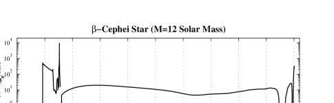
Figure 1: Dimensionless equilibrium quantities including squared buoyancy frequency $N^{2}=(g_{\rm e}/r)A$ with $A=(1/\Gamma_{1})(d\ln p/d\ln x)-(d\ln\rho/d\ln x)$, spherically and non-spherically-symmetric contributions $\rho$ and $\rho_{22}$ to the density, and non-spherically-symmetric gravitational-potential contribution $\phi_{22}$, in units of $GM/R^{3}$, $\rho_{\rm c}$ and $R^{2}\bar{\Omega}^{2}$, respectively, against fractional radius $x=r/R$ for a $\beta$-Cephei star model with $M=12M_{\odot}$.

In order to calculate the effect of rotation on normal modes, I consider a uniformly rotating, 12 $M_{\odot}$, $\beta$ Cephei model generated by the evolution code of Christensen-Dalsgaard (1982) (see also Christensen-Dalsgaard & Thompson 1999). The parameters of the model are listed at Table 1. The value of central hydrogen abundance and existence of small convective core show that the model should be a quite evolved $\beta$-Cephei star. The behavior of some of equilibrium quantities of the model against fractional radius, $x=r/R$ are represented in Fig. 1; It shows that: 1) Close to the center up to radius $x=0.1$, the star is in a convective regime where squared buoyancy frequency $N^{2}<0$ and, outside of this radius is in a radiative regime where $N^{2}>0$. There is a sharp peak in $N^{2}$ at $x\simeq 0.15$. This happens because on one hand $N^{2}\propto g_{e}$ and on the other hand since the model has a very small convective core, $R_{\rm{conv}}=0.1~{}R$, hence the gravity, $g_{e}$, increases sharply. 2) Spherically symmetric density $\rho$ decreases smoothly from its maximum value to nearly zero near the surface at $x\simeq 0.4$; 3) The absolute value of the non-spherically-symmetric correction to the density $\rho_{22}$, see Eq. (10) in Paper I, does show a sharp peak at $x\simeq 0.15$; 4) The absolute value of the non-spherically-symmetric correction to the gravitational potential $\phi_{22}$, see Eq. (12) in Paper I, increases smoothly to its maximum value at the surface.

2.1 Eigenfunctions

The zero-order eigenfunctions are computed from the zero order eigenvalue problem with the pulsation code of Christensen-Dalsgaard (see Christensen-Dalsgaard & Berthomieu 1991), modified according to Eqs. (20) to (24) in Paper I.

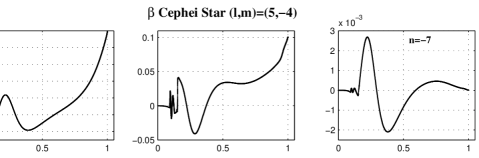
Figure 2: Zero-order radial $y$ (left) and horizontal $z$ components (middle) as well as $r\rho^{1/2}\xi_{r}/(R^{2}\rho_{\rm c}^{1/2})$, related to the energy density (right), against fractional radius $x=r/R$ for selected g-modes with $(l,m)=(5,-4)$ and $n=(-7,-8,-9,-10,-11)$ for the model described in Table 1.

In Fig. 2, the radial ($y$) and horizontal ($z$) components of the zero-order poloidal eigenfunctions as well as $r\rho^{1/2}\xi_{r}/(R^{2}\rho_{\rm c}^{1/2})$ related to the radial energy density, where $\xi_{r}=ry$ is the radial displacement, are plotted against the fractional radius $x=r/R$ for the selected modes with $(l,m)$=(5,-4) and $n$=(-7,…,-11). The modes with $n=(-8,-10)$ are the pure g-modes and with $n=(-7,-9,-11)$ are the mixed g-modes. For the pure g-modes, the oscillations are mostly trapped near the center and also the horizontal amplitude of oscillations are comparable against the radial component. The horizontal component of buoyancy force which generates the horizontal amplitude, plays a important rule during the oscillation of a pure g-mode. At mathematical point of view a pure g-mode is mostly derived from a vector potential that its horizontal component has essential contribution in contrast with the corresponding radial component. This feature is clear particularly for polytropic models. See Sobouti (1980) and Sobouti $\&$ Rezania (2001). In the case of mixed g-modes, the oscillations are trapped between near the center and the middle part of the star. However the amplitude near the surface is decayed exponentially. Figure 2 also shows that: 1) The rapid oscillations in the pure and the mixed g-modes, occur at $x=0.1$ due to existence of sharp peak in squared buoyancy frequency $N^{2}$ (see also Fig. 1). 2) Close to the center up to radius $x=0.1$, where the star is in convective regime ($N^{2}<0$), the amplitudes of modes are decayed exponentially (see again Fig. 1).

2.2 Eigenfrequencies and corrections

The zero-order eigenfrequency, $\sigma_{0}$, is derived from numerical solutions of Eqs. (20) to (24) in Paper I by the modified pulsation code; note that using the eigensystem in Eqs. (20) to (24) the first-order frequency correction, $\sigma_{1}$, is implicitly included in $\sigma_{0}$ (see Eqs. (15) and (16) in Paper I). The second- and third-order Coriolis contributions, ($\sigma_{2}^{\rm T},~{}\sigma_{3}^{\rm T}$), the second- and third-order non-spherically-symmetric distortions, ($\sigma_{2}^{\rm D},~{}\sigma_{3}^{\rm D}$), and the third-order distortion and Coriolis coupling, $\sigma_{3}^{\rm C}$, are derived from numerical integrations of Eqs. (52), (53), (64), (65), and (69) in Paper I.

In Tables 2 to 9 the results of different contributions of frequency corrections due to effect of rotation up to third order are tabulated. In each table the selected p, f and g modes with $(l,m)=(5,-4)$, $(2,0)$, $(2,1)$, $(2,2)$, $(2,-1)$, $(5,0)$, $(5,1)$, and $(5,4)$ with $n=(-3,\ldots,-20)$, $(1,\ldots,-5)$, $(1,\ldots,-5)$, $(1,\ldots,-4)$, $(1,\ldots,-5)$, $(-2,\ldots,-11)$, $(-1,\ldots,-10)$, and $(0,\ldots,-7)$, respectively, are considered. The modes with $n\geq 1$, $n=0$, and $n<0$ are labelled by $({\rm p}_{1},\ldots,{\rm p}_{n})$, f, and $(g_{1},...,g_{n})$, respectively.

Tables 2 to 9 show that: 1) The values of zero order eigenfrequency, $\sigma_{0}$, and total frequency, $\sigma_{\rm tot}$, decrease when the radial mode number, $n$, decreases. 2) The order of magnitudes of ($\sigma_{2}^{D}$, $\sigma_{3}^{D}$) are smaller than ($\sigma_{2}^{T}$, $\sigma_{3}^{T}$) by a factor of $10^{-3}$ to $10^{-1}$. Therefore one can concludes that the effect of Coriolis forces is dominant with respect to the centrifugal forces. 3) With increasing $n$, the frequency correction due to the distortion and the Coriolis coupling increases and decreases alternatively. 4) For the case of $m=0$, there is no first and third-order frequency corrections.

In Table 10, the results of third order frequency corrections for the case of two near degenerate modes, derived from Eqs. (75)-(76), are tabulated. The coupling exists only for the two near degenerate modes belonging to the same $m$ but $l$ differing by $\pm 2$. However there is no any selection rule for $n$.

Note that in the numerical calculations, there are two substantial differences between the equations used in Soufi et al. (1998) and Paper I. In the formulation of Soufi et al. (1998), the density derivatives are eliminated through an integration by parts and the resulting surface terms are ignored. The surface terms become significant for higher-order modes, particularly in the present model whose atmosphere is relatively thin. The other important difference which should be noted is that in Soufi et al. (1998) for computing the third-order correction terms the approximation $z\simeq y_{t}/C\sigma_{0}^{2}$, which is valid for the non-rotating case, is used. In Paper I, on the other hand, the exact relation Eq. (24) is used. The approximation of neglecting the second term in Eq. (24) everywhere, particularly near the surface, is not valid. The magnitude of this difference between the two approaches is more significant than the magnitude of the difference due to of the surface terms for the present model. If we include the surface terms in Soufi et al. (1998) and use the approximation $z\simeq y_{t}/C\sigma_{0}^{2}$ in Paper I, the results of the two numerical approaches are in good agreement.

3 Concluding remarks

The third-order effect of rotation on the p, f and g modes for a uniformly rotating $\beta$-Cephei star of mass 12 $M_{\odot}$ has been investigated. The third-order perturbation formalism presented by Soufi et al. (1998) and revised by Karami (2008) was used. The zero-order eigenvalue problem was solved by pulsation code modified in this manner. Numerical calculations of oscillation frequencies were carried out for our selected model and second- and third-order frequency corrections due to Coriolis, non-spherically-symmetric distortion and Coriolis-distortion coupling were computed. For the case of $m=0$, there is no first and third-order frequency corrections. Coupling only occurs between two poloidal modes with the same $m$ and with $l$ differing by 0 or 2.

Acknowledgements This work was supported by the Research Institute for Astronomy $\&$ Astrophysics of Maragha (RIAAM), Maragha, Iran. I wish to thank Prof. Christensen-Daslgaard for given the model.

Table 1: Stellar parameters of a rotating $\beta$-Cephei star in solar units. $M$, $M_{\rm conv}$, $R$, $R_{\rm conv}$, $p_{\rm c}$, and $\rho_{\rm c}$ are the total mass, the mass of convective core, the radius, the radius of convective core, the central pressure and density, and $\odot$ denotes solar values; $\sigma_{\bar{\Omega}}$ and $\epsilon$ are the dimensionless mean angular velocity and the perturbational expansion coefficient; $T_{\rm dyn}$, $T_{\rm rot}$, and $V_{\rm rot}$ are the dynamical time scale (free fall time), the equatorial period and velocity, respectively. For comparison note that $T_{\odot\rm dyn}=0.5~{}\rm h$, $T_{\odot\rm rot}=25~{}\rm d$, $V_{\odot\rm rot}=2~{}\rm km\,s^{-1}$. $X_{\rm{c}}$ is central helium abundance.

$M=12~{}M_{\odot}$	$M_{\rm{conv}}=0.18~{}M$
$R=8.92~{}R_{\odot}$	$R_{\rm{conv}}=0.1~{}R$
$P_{\rm{c}}=2.85\times 10^{-1}~{}P_{\rm{c}\odot}$	$\rho_{\rm{c}}=5.39\times 10^{-2}~{}\rho_{\rm{c}\odot}$
$\sigma_{\bar{\Omega}}=1.78\times 10^{-1}$	$\epsilon=\Omega/\omega=\sigma_{\bar{\Omega}}/2\pi=2.84\times 10^{-2}$
$T_{\rm{dyn}}=\sqrt{R^{3}/GM}=3.41~{}\rm{h}$	$T_{\rm{rot}}=2\pi R/V_{\rm{rot}}=4.94~{}\rm{d}$
$V_{\rm{rot}}=R\Omega=R\sigma_{\bar{\Omega}}/T_{\rm{dyn}}=90~{}\rm{km/sec}$	$X_{\rm{c}}=0.3$

Table 2: Values of eigenfrequency $\sigma_{0}$ (including the $O(\Omega)$ contribution from rotation), second- and third-order Coriolis contributions $\sigma_{2}^{\rm T}$ and $\sigma_{3}^{\rm T}$, second- and third-order non-spherically-symmetric distortions $\sigma_{2}^{\rm D}$ and $\sigma_{3}^{\rm D}$, third-order distortion and Coriolis coupling $\sigma_{3}^{\rm C}$, and total frequency $\sigma_{\rm tot}=\sigma_{0}+\sigma_{\rm c}$ corrected up to third order, for g modes in a $\beta$-Cephei star with $M=12M_{\odot}$, $(l,m)=(5,-4)$ and $n=(-3,...,-20)$. Here $\sigma_{\rm c}=\sigma_{2}^{\rm T}+\sigma_{3}^{\rm T}+\sigma_{2}^{\rm D}+\sigma_{3}^{\rm D}+\sigma_{3}^{\rm C}$ is the total third-order frequency correction. All frequencies are in units of $\sqrt{GM/R^{3}}=8.16\times 10^{-5}Hz$.

$Mode$	$n$	$\sigma_{0}$	$\sigma_{2}^{\rm T}$	$\sigma_{2}^{\rm D}$	$\sigma_{3}^{\rm T}$	$\sigma_{3}^{\rm D}$	$\sigma_{3}^{\rm C}$	$\sigma_{\rm tot}$
${\rm g}_{3}$	-3	4.8665	2.8674$\times 10^{-3}$	-3.4879$\times 10^{-5}$	4.3614$\times 10^{-4}$	-4.9596$\times 10^{-6}$	1.3462$\times 10^{-6}$	4.8698
${\rm g}_{4}$	-4	4.4391	3.4832$\times 10^{-3}$	-7.1841$\times 10^{-4}$	6.1277$\times 10^{-4}$	-1.1948$\times 10^{-4}$	-1.5434$\times 10^{-5}$	4.4423
${\rm g}_{5}$	-5	4.1259	2.9132$\times 10^{-3}$	-2.6820$\times 10^{-3}$	4.8904$\times 10^{-4}$	-4.1290$\times 10^{-4}$	-2.1143$\times 10^{-4}$	4.1260
${\rm g}_{6}$	-6	3.7477	3.6829$\times 10^{-3}$	-2.5672$\times 10^{-5}$	7.2645$\times 10^{-4}$	-4.7331$\times 10^{-6}$	1.4759$\times 10^{-6}$	3.7521
${\rm g}_{7}$	-7	3.5272	4.1565$\times 10^{-3}$	-2.7378$\times 10^{-4}$	8.9898$\times 10^{-4}$	-5.5731$\times 10^{-5}$	6.8240$\times 10^{-6}$	3.5319
${\rm g}_{8}$	-8	3.0656	4.4603$\times 10^{-3}$	-2.1286$\times 10^{-5}$	1.0752$\times 10^{-3}$	-4.7965$\times 10^{-6}$	1.8142$\times 10^{-6}$	3.0711
${\rm g}_{9}$	-9	2.9902	4.8440$\times 10^{-3}$	-2.1802$\times 10^{-4}$	1.2330$\times 10^{-3}$	-5.2212$\times 10^{-5}$	2.4225$\times 10^{-5}$	2.9960
${\rm g}_{10}$	-10	2.6251	5.1634$\times 10^{-3}$	-2.1897$\times 10^{-5}$	1.4538$\times 10^{-3}$	-5.7636$\times 10^{-6}$	2.5355$\times 10^{-6}$	2.6317
${\rm g}_{11}$	-11	2.6036	5.4569$\times 10^{-3}$	-2.0487$\times 10^{-4}$	1.5863$\times 10^{-3}$	-5.5969$\times 10^{-5}$	3.2563$\times 10^{-5}$	2.6104
${\rm g}_{12}$	-12	2.3195	5.9638$\times 10^{-3}$	-1.6175$\times 10^{-4}$	1.9283$\times 10^{-3}$	-4.9058$\times 10^{-5}$	3.1539$\times 10^{-5}$	2.3272
${\rm g}_{13}$	-13	2.3148	5.8630$\times 10^{-3}$	-7.2840$\times 10^{-5}$	1.8818$\times 10^{-3}$	-2.1884$\times 10^{-5}$	1.3520$\times 10^{-5}$	2.3224
${\rm g}_{14}$	-14	2.1043	6.5490$\times 10^{-3}$	-2.4611$\times 10^{-4}$	2.3402$\times 10^{-3}$	-8.2550$\times 10^{-5}$	5.7688$\times 10^{-5}$	2.1129
${\rm g}_{15}$	-15	2.0946	6.3502$\times 10^{-3}$	-2.2490$\times 10^{-5}$	2.2402$\times 10^{-3}$	-7.4183$\times 10^{-6}$	4.0019$\times 10^{-6}$	2.1032
${\rm g}_{16}$	-16	1.9432	7.0212$\times 10^{-3}$	-3.5406$\times 10^{-4}$	2.7160$\times 10^{-3}$	-1.2856$\times 10^{-4}$	9.5675$\times 10^{-5}$	1.9526
${\rm g}_{17}$	-17	1.9303	6.8267$\times 10^{-3}$	-2.1125$\times 10^{-5}$	2.6127$\times 10^{-3}$	-7.5594$\times 10^{-6}$	4.2244$\times 10^{-6}$	1.9398
${\rm g}_{18}$	-18	1.8239	7.3883$\times 10^{-3}$	-5.0673$\times 10^{-4}$	3.0403$\times 10^{-3}$	-1.9568$\times 10^{-4}$	1.5051$\times 10^{-4}$	1.8338
${\rm g}_{19}$	-19	1.8162	7.2322$\times 10^{-3}$	-8.5508$\times 10^{-5}$	2.9485$\times 10^{-3}$	-3.2616$\times 10^{-5}$	2.3645$\times 10^{-5}$	1.8263
${\rm g}_{20}$	-20	1.7479	7.4410$\times 10^{-3}$	-2.2532$\times 10^{-5}$	3.1447$\times 10^{-3}$	-8.9049$\times 10^{-6}$	5.1061$\times 10^{-6}$	1.7585

Table 3: Same as Table 2, for p, f and g modes with $(l,m)=(2,0)$ and $n=(1,\ldots,-5)$. There is no $\sigma_{3}^{\rm T}$, $\sigma_{3}^{\rm D}$, and $\sigma_{3}^{\rm C}=0$ for $m=0$ (see Eqs. (53), (65), and (69) in Paper I).

$Mode$	$n$	$\sigma_{0}$	$\sigma_{2}^{\rm T}$	$\sigma_{2}^{\rm D}$	$\sigma_{\rm tot}$
$p_{1}$	1	5.0537	5.5170$\times 10^{-3}$	4.9610$\times 10^{-3}$	5.0642
$f$	0	4.3575	6.4970$\times 10^{-3}$	3.6577$\times 10^{-3}$	4.3677
$g_{1}$	-1	4.0537	6.8344$\times 10^{-3}$	1.1652$\times 10^{-3}$	4.0617
$g_{2}$	-2	3.3908	8.3406$\times 10^{-3}$	2.5483$\times 10^{-3}$	3.4016
$g_{3}$	-3	2.8396	9.6665$\times 10^{-3}$	1.5772$\times 10^{-4}$	2.8494
$g_{4}$	-4	2.2565	1.2362$\times 10^{-2}$	3.0039$\times 10^{-4}$	2.2691
$g_{5}$	-5	1.9548	1.4006$\times 10^{-2}$	3.7784$\times 10^{-5}$	1.9688

Table 4: Same as Table 2, for p, f and g modes with $(l,m)=(2,1)$ and $n=(1,\ldots,-5)$.

$Mode$	$n$	$\sigma_{0}$	$\sigma_{2}^{\rm T}$	$\sigma_{2}^{\rm D}$	$\sigma_{3}^{\rm T}$	$\sigma_{3}^{\rm D}$	$\sigma_{3}^{\rm C}$	$\sigma_{\rm tot}$
$p_{1}$	1	4.9013	4.8280$\times 10^{-3}$	1.3791$\times 10^{-3}$	-2.4142$\times 10^{-4}$	-4.2330$\times 10^{-5}$	-1.0047$\times 10^{-4}$	4.9072
$f$	0	4.2006	5.7720$\times 10^{-3}$	1.2503$\times 10^{-3}$	-3.3610$\times 10^{-4}$	-4.6251$\times 10^{-5}$	-8.0721$\times 10^{-5}$	4.2071
$g_{1}$	-1	3.9018	6.1250$\times 10^{-3}$	3.9277$\times 10^{-4}$	-3.8355$\times 10^{-4}$	-1.5264$\times 10^{-5}$	-2.7455$\times 10^{-5}$	3.9079
$g_{2}$	-2	3.2352	7.4881$\times 10^{-3}$	1.1421$\times 10^{-3}$	-5.6654$\times 10^{-4}$	-5.3947$\times 10^{-5}$	-7.4684$\times 10^{-5}$	3.2431
$g_{3}$	-3	2.6895	9.0188$\times 10^{-3}$	7.0794$\times 10^{-5}$	-8.2311$\times 10^{-4}$	-3.9603$\times 10^{-6}$	-9.7091$\times 10^{-6}$	2.6977
$g_{4}$	-4	2.1013	1.2036$\times 10^{-2}$	1.3298$\times 10^{-4}$	-1.4124$\times 10^{-3}$	-9.8793$\times 10^{-6}$	-3.9305$\times 10^{-5}$	2.1120
$g_{5}$	-5	1.8055	1.3823$\times 10^{-2}$	1.8283$\times 10^{-5}$	-1.8938$\times 10^{-3}$	-1.5144$\times 10^{-6}$	-5.6319$\times 10^{-6}$	1.8174

Table 5: Same as Table 2, for p, f and g modes with $(l,m)=(2,2)$ and $n=(1,\ldots,-4)$.

$Mode$	$n$	$\sigma_{0}$	$\sigma_{2}^{\rm T}$	$\sigma_{2}^{\rm D}$	$\sigma_{3}^{\rm T}$	$\sigma_{3}^{\rm D}$	$\sigma_{3}^{\rm C}$	$\sigma_{\rm tot}$
$p_{1}$	1	4.7531	1.5883$\times 10^{-3}$	-6.2091$\times 10^{-4}$	-1.1783$\times 10^{-4}$	3.8294$\times 10^{-5}$	3.9523$\times 10^{-4}$	4.7544
$f$	0	4.0472	2.1026$\times 10^{-3}$	-1.2523$\times 10^{-3}$	-1.8862$\times 10^{-4}$	9.3932$\times 10^{-5}$	3.2290$\times 10^{-4}$	4.0483
$g_{1}$	-1	3.7510	2.2968$\times 10^{-3}$	-4.5920$\times 10^{-4}$	-2.2129$\times 10^{-4}$	3.6960$\times 10^{-5}$	7.1757$\times 10^{-5}$	3.7527
$g_{2}$	-2	3.0857	2.6160$\times 10^{-3}$	-1.9895$\times 10^{-3}$	-2.9955$\times 10^{-4}$	1.8946$\times 10^{-4}$	2.3278$\times 10^{-4}$	3.0864
$g_{3}$	-3	2.5394	3.4410$\times 10^{-3}$	-1.2564$\times 10^{-4}$	-4.8923$\times 10^{-4}$	1.4920$\times 10^{-5}$	6.5731$\times 10^{-6}$	2.5422
$g_{4}$	-4	1.9447	5.0666$\times 10^{-3}$	-2.3100$\times 10^{-4}$	-9.7698$\times 10^{-4}$	3.7477$\times 10^{-5}$	8.6389$\times 10^{-6}$	1.9486

Table 6: Same as Table 2, for p, f and g modes with $(l,m)=(2,-1)$ and $n=(1,\ldots,-5)$.

$Mode$	$n$	$\sigma_{0}$	$\sigma_{2}^{\rm T}$	$\sigma_{2}^{\rm D}$	$\sigma_{3}^{\rm T}$	$\sigma_{3}^{\rm D}$	$\sigma_{3}^{\rm C}$	$\sigma_{\rm tot}$
$p_{1}$	1	5.2102	4.4006$\times 10^{-3}$	3.6153$\times 10^{-3}$	2.0474$\times 10^{-4}$	1.1001$\times 10^{-4}$	3.5096$\times 10^{-5}$	5.2186
$f$	0	4.5176	5.1223$\times 10^{-3}$	2.3647$\times 10^{-3}$	2.7408$\times 10^{-4}$	8.4565$\times 10^{-5}$	2.8493$\times 10^{-5}$	4.5255
$g_{1}$	-1	4.2071	5.2688$\times 10^{-3}$	7.9315$\times 10^{-4}$	3.0026$\times 10^{-4}$	2.9067$\times 10^{-5}$	1.7027$\times 10^{-5}$	4.2135
$g_{2}$	-2	3.5517	6.5049$\times 10^{-3}$	1.3879$\times 10^{-3}$	4.4055$\times 10^{-4}$	6.3833$\times 10^{-5}$	3.9379$\times 10^{-5}$	3.5601
$g_{3}$	-3	2.9898	7.1166$\times 10^{-3}$	8.6542$\times 10^{-5}$	5.6663$\times 10^{-4}$	4.3428$\times 10^{-6}$	1.0038$\times 10^{-5}$	2.9976
$g_{4}$	-4	2.4105	8.8416$\times 10^{-3}$	1.6696$\times 10^{-4}$	8.7025$\times 10^{-4}$	1.0610$\times 10^{-5}$	4.4664$\times 10^{-5}$	2.4204
$g_{5}$	-5	2.1045	9.8081$\times 10^{-3}$	1.9592$\times 10^{-5}$	1.1018$\times 10^{-3}$	1.3914$\times 10^{-6}$	6.6382$\times 10^{-6}$	2.1154

Table 7: Same as Table 3, for g modes with $(l,m)=(5,0)$ and $n=(-2,\ldots,-11)$.

$Mode$	$n$	$\sigma_{0}$	$\sigma_{2}^{\rm T}$	$\sigma_{2}^{\rm D}$	$\sigma_{\rm tot}$
$g_{2}$	-2	4.6430	6.5692$\times 10^{-3}$	5.1648$\times 10^{-3}$	4.6548
$g_{3}$	-3	4.1745	7.4434$\times 10^{-3}$	4.6698$\times 10^{-5}$	4.1820
$g_{4}$	-4	3.7054	8.6005$\times 10^{-3}$	1.0041$\times 10^{-3}$	3.7150
$g_{5}$	-5	3.4917	8.5212$\times 10^{-3}$	2.4579$\times 10^{-3}$	3.5027
$g_{6}$	-6	3.0567	1.0158$\times 10^{-2}$	3.1727$\times 10^{-5}$	3.0669
$g_{7}$	-7	2.8068	1.1320$\times 10^{-2}$	2.2605$\times 10^{-4}$	2.8184
$g_{8}$	-8	2.3747	1.3073$\times 10^{-2}$	2.4209$\times 10^{-5}$	2.3878
$g_{9}$	-9	2.2732	1.3929$\times 10^{-2}$	1.6712$\times 10^{-4}$	2.2873
$g_{10}$	-10	1.9343	1.6049$\times 10^{-2}$	1.9849$\times 10^{-5}$	1.9504
$g_{11}$	-11	1.8916	1.6674$\times 10^{-2}$	1.3491$\times 10^{-4}$	1.9085

Table 8: Same as Table 2, for g modes with $(l,m)=(5,1)$ and $n=(-1,\ldots,-10)$.

$Mode$	$n$	$\sigma_{0}$	$\sigma_{2}^{\rm T}$	$\sigma_{2}^{\rm D}$	$\sigma_{3}^{\rm T}$	$\sigma_{3}^{\rm D}$	$\sigma_{3}^{\rm C}$	$\sigma_{\rm tot}$
$g_{1}$	-1	5.2735	5.7438$\times 10^{-3}$	7.7440$\times 10^{-5}$	-2.0385$\times 10^{-4}$	-2.5593$\times 10^{-6}$	-7.0613$\times 10^{-7}$	5.2791
$g_{2}$	-2	4.4767	6.5970$\times 10^{-3}$	2.6340$\times 10^{-3}$	-2.6521$\times 10^{-4}$	-9.7601$\times 10^{-5}$	-1.3530$\times 10^{-4}$	4.4855
$g_{3}$	-3	4.0016	7.5499$\times 10^{-3}$	3.9642$\times 10^{-5}$	-3.5099$\times 10^{-4}$	-1.7135$\times 10^{-6}$	-8.7762$\times 10^{-7}$	4.0088
$g_{4}$	-4	3.5245	8.7660$\times 10^{-3}$	8.3310$\times 10^{-4}$	-4.7788$\times 10^{-4}$	-4.2566$\times 10^{-5}$	-3.4359$\times 10^{-5}$	3.5335
$g_{5}$	-5	3.3328	8.6929$\times 10^{-3}$	1.6871$\times 10^{-3}$	-4.5513$\times 10^{-4}$	-8.0691$\times 10^{-5}$	-1.0396$\times 10^{-4}$	3.3426
$g_{6}$	-6	2.8839	1.0492$\times 10^{-2}$	2.6152$\times 10^{-5}$	-6.7611$\times 10^{-4}$	-1.5664$\times 10^{-6}$	-9.6720$\times 10^{-7}$	2.8938
$g_{7}$	-7	2.6261	1.1821$\times 10^{-2}$	1.5839$\times 10^{-4}$	-8.6786$\times 10^{-4}$	-1.0907$\times 10^{-5}$	-7.8477$\times 10^{-6}$	2.6372
$g_{8}$	-8	2.2021	1.3773$\times 10^{-2}$	1.9341$\times 10^{-5}$	-1.1620$\times 10^{-3}$	-1.5166$\times 10^{-6}$	-9.7065$\times 10^{-7}$	2.2147
$g_{9}$	-9	2.0938	1.4799$\times 10^{-2}$	1.0486$\times 10^{-4}$	-1.3547$\times 10^{-3}$	-8.9901$\times 10^{-6}$	-7.3938$\times 10^{-6}$	2.1073
$g_{10}$	-10	1.7617	1.7257$\times 10^{-2}$	1.5214$\times 10^{-5}$	-1.8197$\times 10^{-3}$	-1.4909$\times 10^{-6}$	-9.8237$\times 10^{-7}$	1.7771

Table 9: Same as Table 2, for f and g modes with $(l,m)=(5,4)$ and $n=(0,\ldots,-7)$.

$Mode$	$n$	$\sigma_{0}$	$\sigma_{2}^{\rm T}$	$\sigma_{2}^{\rm D}$	$\sigma_{3}^{\rm T}$	$\sigma_{3}^{\rm D}$	$\sigma_{3}^{\rm C}$	$\sigma_{\rm tot}$
$f$	0	4.9968	2.6949$\times 10^{-3}$	2.9857$\times 10^{-3}$	-3.8428$\times 10^{-4}$	-3.9355$\times 10^{-4}$	2.5204$\times 10^{-4}$	5.0020
$g_{1}$	-1	4.7510	3.0994$\times 10^{-3}$	-4.5756$\times 10^{-5}$	-4.8592$\times 10^{-4}$	6.7139$\times 10^{-6}$	-7.5470$\times 10^{-7}$	4.7535
$g_{2}$	-2	3.9831	3.3532$\times 10^{-3}$	2.5387$\times 10^{-3}$	-5.9624$\times 10^{-4}$	-4.1671$\times 10^{-4}$	3.0860$\times 10^{-4}$	3.9883
$g_{3}$	-3	3.4828	4.1984$\times 10^{-3}$	-2.1823$\times 10^{-5}$	-8.9241$\times 10^{-4}$	4.3348$\times 10^{-6}$	-9.4382$\times 10^{-7}$	3.4861
$g_{4}$	-4	2.9964	4.8000$\times 10^{-3}$	-1.1922$\times 10^{-4}$	-1.1736$\times 10^{-3}$	2.7171$\times 10^{-5}$	1.2330$\times 10^{-4}$	3.0000
$g_{5}$	-5	2.8464	4.8577$\times 10^{-3}$	-1.6612$\times 10^{-4}$	-1.2257$\times 10^{-3}$	3.8867$\times 10^{-5}$	1.0211$\times 10^{-4}$	2.8500
$g_{6}$	-6	2.3658	6.2203$\times 10^{-3}$	-1.2587$\times 10^{-5}$	-1.9446$\times 10^{-3}$	3.6761$\times 10^{-6}$	-9.7763$\times 10^{-7}$	2.3701
$g_{7}$	-7	2.0828	7.6637$\times 10^{-3}$	-1.8813$\times 10^{-5}$	-2.8324$\times 10^{-3}$	6.5530$\times 10^{-6}$	-9.7497$\times 10^{-6}$	2.0876

Table 10: Values of zero-order eigenfrequency $\sigma_{0}$, total frequency $\sigma_{\pm}$ corrected up to third order, total third-order frequency correction $\Delta\sigma_{\pm}=(\sigma_{\pm}-\sigma_{0})$ due to rotation and coupling, expansion coefficients ${\mathcal{A}}_{1}^{(\pm)}$ and ${\mathcal{A}}_{2}^{(\pm)}$ normalized to 1, i.e., ${\mathcal{A}}_{1}^{2}+{\mathcal{A}}_{2}^{2}=1$, for selected pairs of near-degenerate poloidal modes in a $\beta$-Cephei star with $M=12M_{\odot}$. All frequencies are in units of $\sqrt{GM/R^{3}}=8.16\times 10^{-5}Hz$.

$m$	$l$	$n$	coupling	$\sigma_{0}$	$\sigma_{\pm}$	$\Delta\sigma_{\pm}$	${\mathcal{A}}_{1}^{(\pm)}$	${\mathcal{A}}_{2}^{(\pm)}$
0	0	3	$p_{3}$	5.1186	5.1271	8.4915$\times 10^{-3}$	9.98528$\times 10^{-1}$	5.42353$\times 10^{-2}$
0	2	1	$p_{1}$	5.0537	5.0640	1.0282$\times 10^{-2}$	5.72211$\times 10^{-2}$	-9.98362$\times 10^{-1}$
0	2	-2	$g_{2}$	3.3908	3.4016	1.0888$\times 10^{-2}$	9.99999$\times 10^{-1}$	1.65116$\times 10^{-3}$
0	4	-4	$g_{4}$	3.4704	3.4795	9.1303$\times 10^{-3}$	8.92439$\times 10^{-3}$	-9.99960$\times 10^{-1}$
1	3	-3	$g_{3}$	3.3049	3.3141	9.2414$\times 10^{-3}$	9.98573$\times 10^{-1}$	5.34025$\times 10^{-2}$
1	5	-5	$g_{5}$	3.3328	3.3426	9.8344$\times 10^{-3}$	4.56655$\times 10^{-2}$	-9.98957$\times 10^{-1}$
2	3	-3	$g_{3}$	3.1457	3.1511	5.3915$\times 10^{-3}$	9.98319$\times 10^{-1}$	5.79619$\times 10^{-2}$
2	5	-5	$g_{5}$	3.1729	3.1809	8.0497$\times 10^{-3}$	5.62952$\times 10^{-2}$	-9.98414$\times 10^{-1}$
3	3	-3	$g_{3}$	2.9905	2.9908	3.3252$\times 10^{-4}$	9.98752$\times 10^{-1}$	4.99354$\times 10^{-2}$
3	5	-5	$g_{5}$	3.0111	3.0171	5.9922$\times 10^{-3}$	5.81273$\times 10^{-2}$	-9.98309$\times 10^{-1}$

References

- [1] Christensen-Dalsgaard J., 1982, MNRAS, 199, 735
- [2] Christensen-Dalsgaard J., Berthomieu G., 1991, in Solar interior and atmosphere, eds. A. N. Cox, W. C. Livingston, & M. Matthews, Space Science Series, Tucson: University of Arizona Press, 401
- [3] Christensen-Dalsgaard J., Thompson M. J., 1999, A&A, 350, 852
- [4] Daszyńska-Daszkiewicz J., Dziembowski W. A., Pamyatnykh A. A., Goupil M-J., 2002, A&A, 392, 151
- [5] Dziembowski W. A., Goode P. R., 1992, ApJ, 394, 670
- [6] Goupil M. J., Dziembowski W. A., Pamyatnykh A., Talon S., 2001, in Delta Scuti and related stars, eds. M. Breger, & M. H. Montgomery, ASP Conf. Ser., 210, 267
- [7] Goupil M. J., Samadi R., Lochard J., Dziembowski W. A., Pamyatnykh A., 2004, in Stellar structure and habitable planet finding, eds. F. Favata, S. Aigrain & A. Wilson, ESA SP-538, 133
- [8] Goupil M. J., Talon S., 2002, in Radial and Nonradial Pulsations as Probes of Stellar Physics, eds. C. Aerts, T. R. Bedding, & J. Christensen-Dalsgaard, ASP Conf. Ser., 259, 306
- [9] Karami K., Christensen-Dalsgaard J., Pijpers F. P., 2003, in Solar and Solar-Like Oscillations: Insights and Challenges for the Sun and Stars, 25th meeting of the IAU, Joint Discussion 12, Abstract Book, p.213
- [10] Karami K., 2008, ChJAA, 8, 285 (Paper I)
- [11] Pamyatnykh A., 2003, in Astroseismology across the HR diagram, eds. M. J. Thompson, M. S. Cunha, & M. J. P. F. G. Monteiro (Dordrecht: Kluwer), 97 (also Ap. Sp. Sci., 284, 97)
- [12] Reese D., Lignières F., Rieutord M., 2006, A&A, 455, 621
- [13] Sobouti Y., 1980, A&A, 89, 314
- [14] Sobouti Y., Rezania V., 2001, A&A, 375, 680
- [15] Soufi F., Goupil M. J., Dziembowski W. A., 1998, A&A, 334, 911
- [16] Suárez J. C., Goupil M. J., Morel P., 2006, A&A, 449, 673