Modeling He-rich subdwarfs through the hot-flasher scenario

Abstract

We present 1D numerical simulations aimed at studying the hot-flasher scenario for the formation of He-rich subdwarf stars. Sequences were calculated for a wide range of metallicities and with the He core flash at different points of the post-RGB evolution (i.e. different remnant masses). We followed the complete evolution from the ZAMS, through the hot-flasher event, and to the subdwarf stage for all kinds of hot-flashers. This allows us to present a homogeneous set of abundances for different metallicities and all flavors of hot-flashers. We extend the scope of our work by analyzing the effects in the predicted surface abundances of some standard assumptions in convective mixing and the effects of element diffusion.

We find that the hot-flasher scenario is a viable explanation for the formation of He-sdO stars. Our results also show that element diffusion may produce the transformation of (post hot-flasher) He-rich atmospheres into He-deficient ones. If this is so, then the hot-flasher scenario is able to reproduce both the observed properties and distribution of He-sdO stars.

1 Introduction

Hot subdwarf stars can roughly be grouped into the cooler sdB stars, whose spectra display typically no or only weak helium lines, and the hotter sdO stars, which have higher helium abundances on average and can even be dominated by helium. The diversity of spectra observed among sdO stars and the helium-enhanced surface abundances observed in many of these stars (Lemke et al. 1997) pose a challenge to stellar evolution theory. As a consequence, some non-canonical evolutionary scenarios were proposed to explain the formation of He-rich subdwarf stars (i.e. He-sdB, He-sdO stars). Among them, the merger of two white dwarfs (Saio & Jeffery 2000) and a helium core flash (HeCF) after departure from the red giant branch (i.e. “hot-flasher scenario”; D’Cruz et al. 1996, Sweigart 1997) offer the most promising explanations of their formation (Ströer et al. 2007). The hot-flasher scenario was also proposed to explain the existence and characteristics of blue hook stars in some globular clusters (see Moehler et al. 2007 and references therein). Following Lanz et al. (2004) hot-flashers can be classified into early hot-flashers, which experience the HeCF during the evolution at constant luminosity (after departure from the RGB) and become hot subdwarfs with standard H/He envelopes; and late hot-flashers, which end as He-enriched hot subdwarfs either by burning or dilution of the remaining H-rich envelope. The latter case is the object of the present article.

2 Description of the present work

The core feature of this work is to present a homogeneous set of simulations of the late hot-flasher scenario (i.e. those events that lead to He-enhanced stellar surfaces) for which the chemical abundances are consistently calculated by simultaneously solving the mixing and burning equations within a diffusive convection picture. We then extend the scope of this work by analyzing how these results can be altered by some non-standard assumptions, such as deviations from the standard mixing length theory (MLT) or element diffusion. Particular emphasis is placed on on the predicted surface properties of the models.

The sequences presented in this work were calculated with LPCODE, a numerical code for solving the equations of stellar structure which is extensively described in Althaus et al. (2005).

In our simulations we have followed the evolution from the ZAMS, through the hot-flasher event and then to the He-core burning stage. Simulations of the hot-flasher scenario were performed for 4 different metallicities and with the HeCF taking place at different points of the post-RGB evolution (which corresponds to different remnant masses, see Table 1). Initial masses and abundances are shown on Table 1 together with the range of post-RGB remnant masses for which He-enriched subdwarfs are obtained.

Mass at ZAMS	Initial Abundances	Remnant mass range
($M_{\odot}$)	(X0/Y0/Z0)	for late hot-flashers ($M_{\odot}$)
0.88	0.769/0.230/0.001	0.4916 — 0.4810
0.98	0.736/0.254/0.010	0.4780 — 0.4662
1.03	0.702/0.278/0.020	0.4740 — 0.4611
1.04	0.668/0.302/0.030	0.4658 — 0.4522

Table 1: Initial (ZAMS) values of our standard sequences and range of remnant masses in which late hot-flashers are obtained.

For a more extensive discussion on the numerical and physical aspects of the models, as well as on the results of the present study, we refer the reader to Miller Bertolami et al. (2008).

3 Results and discussion

Final Mass [$M_{\odot}$]	Z0	H	He	12C	13C	N	O
0.49145 (SM∗)	0.001	0.2137	0.7475	0.0365	$1.57\times 10^{-6}$	$1.22\times 10^{-4}$	$1.52\times 10^{-3}$
0.49104 (DM)	0.001	$2.42\times 10^{-4}$	0.9450	0.0267	$7.47\times 10^{-3}$	0.0106	$4.77\times 10^{-5}$
0.48545 (DM)	0.001	$4.60\times 10^{-6}$	0.9524	0.0264	$7.73\times 10^{-3}$	0.0134	$4.53\times 10^{-5}$
0.48150 (DM)	0.001	$2.41\times 10^{-6}$	0.9666	0.0107	$5.79\times 10^{-3}$	0.0185	$3.79\times 10^{-5}$
0.47770 (SM)	0.01	0.0780	0.8682	0.0426	$6.26\times 10^{-6}$	$1.30\times 10^{-3}$	$6.84\times 10^{-4}$
0.47744 (SM∗)	0.01	0.0261	0.8996	0.0642	$2.36\times 10^{-6}$	$6.59\times 10^{-4}$	$7.43\times 10^{-4}$
0.47725 (DM)	0.01	$2.27\times 10^{-5}$	0.9464	0.0382	$6.12\times 10^{-3}$	$4.35\times 10^{-3}$	$2.94\times 10^{-4}$
0.46921 (DM)	0.01	$1.02\times 10^{-5}$	0.9560	0.0211	$6.13\times 10^{-3}$	0.0128	$2.92\times 10^{-4}$
0.46644 (DM)	0.01	$4.61\times 10^{-6}$	0.9592	0.0193	$5.52\times 10^{-3}$	0.0122	$3.16\times 10^{-4}$
0.47378 (SM)	0.02	0.3822	0.5978	$1.23\times 10^{-3}$	$8.96\times 10^{-5}$	$7.57\times 10^{-3}$	$4.69\times 10^{-3}$
0.47250 (SM∗)	0.02	$9.56\times 10^{-3}$	0.9273	0.0425	$1.93\times 10^{-5}$	$2.94\times 10^{-3}$	$8.64\times 10^{-4}$
0.47112 (DM)	0.02	$9.05\times 10^{-6}$	0.9389	0.0420	$4.27\times 10^{-3}$	$4.88\times 10^{-3}$	$6.96\times 10^{-4}$
0.46410 (DM)	0.02	$1.05\times 10^{-5}$	0.9460	0.0273	$6.41\times 10^{-3}$	0.0120	$7.680\times 10^{-4}$
0.46150 (DM)	0.02	$4.66\times 10^{-6}$	0.9480	0.0263	$5.67\times 10^{-3}$	0.0116	$1.01\times 10^{-3}$
0.46521 (SM)	0.03	0.2227	0.7271	0.0197	$7.79\times 10^{-5}$	$8.09\times 10^{-3}$	$5.18\times 10^{-3}$
0.46470 (SM)	0.03	$4.71\times 10^{-3}$	0.9239	0.0380	$4.12\times 10^{-4}$	$6.10\times 10^{-3}$	$1.58\times 10^{-3}$
0.46367 (SM∗)	0.03	$1.63\times 10^{-3}$	0.9249	0.0390	$3.25\times 10^{-3}$	$6.48\times 10^{-3}$	$1.62\times 10^{-3}$
0.46282 (DM)	0.03	$7.48\times 10^{-6}$	0.9333	0.0420	$1.74\times 10^{-3}$	$7.04\times 10^{-3}$	$1.55\times 10^{-3}$
0.45660 (DM)	0.03	$9.22\times 10^{-6}$	0.9382	0.0341	$4.09\times 10^{-3}$	0.0103	$1.67\times 10^{-3}$
0.45234 (DM)	0.03	$1.94\times 10^{-5}$	0.9411	0.0273	$4.76\times 10^{-3}$	0.0134	$2.14\times 10^{-3}$

Table 2: Surface abundances (by mass fractions) for sequences calculated in this work.

Standard sequences: Convection in our standard sequences is described by the standard MLT with convective boundaries given by a bare Schwarzschild criterium. H-deficiency in our standard sequences is attained by dilution and/or burning of the remaining H-rich envelope, depending on the exact moment of the post-RGB evolution at which the HeCF takes place. If the star is already at the WD cooling track when the HeCF develops (deep mixing events; DM) then the convective zone generated by the HeCF is able to penetrate into the H-rich envelope and H is violently burned (a H-flash), before the remaining H-envelope is diluted by a very shallow convective zone. On the other hand, if the H-burning shell is still active when the HeCF develops then, the convective zone generated during the HeCF does not reach the H-rich envelope and no H-burning happens. In these cases (shallow mixing events; SM) a mild H-deficiency can be attained when one of the convective zones generated by the HeCF moves towards the H-He transition and merges with a inwardly growing convective envelope. In our simulations there are some transition cases (labelled SM^∗ in Table 2) in which the HeCF driven convective zone partially penetrates into the H-rich envelope, and some H-burning takes place, but no H-flash finally developes. Then H-deficiency is attained by a combination of burning and dilution of the H-rich envelope.

In Table 2 we present the surface abundances for selected sequences calculated in this work. As it is shown in Table 2, DM episodes predict immediately after the flash an extremely H deficient surface with H-abundances preferentially between $10^{-5}$ and $10^{-6}$ (by mass fraction), while SM/SM^∗ predict a more wide range of H-abundances between almost solar and $10^{-3}$.

Although evolutionary tracks pass close to the location of He-sdO stars (see Figure 1), their distribution in the $\log g-\log T_{\rm eff}$ diagram is not correctly reproduced. In fact, according to (standard) theoretical predictions, He-sdO should cluster around the He-core burning stage where evolutionary timescales are longer. However, this inconsistency can be solved when taking into account the effects of element diffusion in the outer layers (see next paragraphs).

Effects of departures from the standard MLT: we have performed additional simulations including the effects of extramixing at convective boundaries (as in Herwig et al. 1997) and/or the effects of chemical gradients (as in Grossman & Taam 1996). Our results show that the role of chemical gradients as an extra barrier to the penetration of the He-core flash driven convective zone into the H-rich envelope, is significant and has to be studied in detail (probably by means of hydrodynamical simulations of the event). In fact, in our simulations, the stabilizing effect of chemical gradients can even prevent the penetration when no extramixing is considered at convective boundaries. On the other hand, extramixing processes alone does not produce significant departures from standard results.

Effects of element diffusion on the outer layers: Recently, Unglaub (2008) showed that chemical homogeneous winds in these stars are not possible at $\log g>5.5$ and, consequently, H and He can hardly be expelled from the stars. In view of these results we have performed simulations of element diffusion in the absence of mass loss by means of the method described in Unglaub & Bues (1998). Figure 1 shows the evolution of the surface abundaces predicted for two of our sequences due to the effects of element diffusion. As it is shown in Figure 1 in the absence of mass loss the SM^∗ sequence becomes H-dominated almost instantly, compared to the evolutionary timescale, and its surface is expected to become H-dominated as soon as homogeneous winds halt. On the other hand for the DM sequence the timescale in which the star becomes H-dominated is similar to the evolutionary timescale from the primary HeCF to the settlement on the He-core burning stage ($\sim 1$ Myr). In this case, the surface is expected to become H-dominated as soon as the He-core burning stage begins and evolutionary timescales become $\sim 40$ times longer. Note that, with the inclusion of element diffusion, the surface properties and distribution of He-sdO stars predicted by the hot-flasher scenario correctly reproduces the observed ones (see Figure 1).

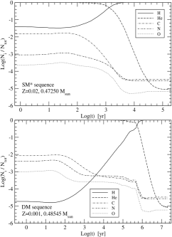
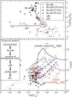
Figure 1: Left: Evolution of the surface ($\tau_{\rm Rosseland}=2/3$) abundances predicted in two of our hot-flashers due to the effects of element diffusion in the absence of mass loss and assuming $T_{\rm eff}=40\,000$ K and $\log g=6$. Bottom Right: Evolution of the same two hot-flasher sequences in the $\log g-\log T_{\rm eff}$ diagram. Thick dashed lines mark the wind limit, for two different metallicities, below which homogeneous winds are not possible according to Unglaub (2008). Dotted lines denoted the portion of the evolutionary track where the star should have already became H-deficient according to element diffusion simulations. Top Right: Sketch of the possible evolution in the $\log N_{\rm He}/N_{\rm H}-\log T_{\rm eff}$ diagram after a deep mixing event.

Part of this work was supported by PIP 6521 grant from CONICET. Also the European Association for Research in Astronomy is acknowledged for an EARA-EST fellowship under which this work was started.

References

Althaus, L. G., Serenelli, A. M., Panei, J. A., et al. 2005, A&A, 435, 631

Cassisi, S., Schlattl, H., Salaris, M., Weiss, A. 2003, ApJL, 582, L43

D’Cruz, N., Dorman, B., Rood, R., O’Connell, R. 1996, ApJ, 466, 359

de Boer, K., Drilling, J., Jeffery, C. & Sion, E. 1997, Third Conference on Faint Blue Stars, L. Davis Press, 515

Grossman, S & Taam, R. 1996, MNRAS, 283, 1165

Herwig, F., Blöcker, T., Schönberner, D. & El Eid, M. 1997, A&A, 324, L81

Lanz, T., Brown, T., Sweigart, A., Hubeny, I., Landsman, W. 2004, ApJ, 602, 342

Lemke, M., Heber, U., Napiwotzki, R., et al. 1997, Third Conference on Faint Blue Stars, L. Davis Press, 375

Miller Bertolami, M. M., Althaus, L. G., Unglaub, K., & Weiss, A. 2008, A&A, DOI: 10.1051/0004-6361:200810373

Moehler, S., Dreizler, S., Lanz, T., et al. 2007, A&A, 475, L5

Saio, H. & Jeffery, S. 2000, MNRAS, 313, 671

Ströer, A., Heber, U., Lisker, T., et al. 2007, A&A, 462, 269

Sweigart, A. 1997, Third Conference on Faint Blue Stars, L. Davis Press, 3

Unglaub, K. 2008, A&A, 486, 923

Unglaub, K. & Bues, I. 1998, A&A, 338, 75