Embedding approach for dynamical mean field theory of strongly correlated heterostructures

Abstract

We present an embedding approach based on localized basis functions which permits an efficient application of the dynamical mean field theory (DMFT) to inhomogeneous correlated materials, such as semi-infinite surfaces and heterostructures. In this scheme, the semi-infinite substrate leads connected to both sides of the central region of interest are represented via complex, energy-dependent embedding potentials that incorporate one-electron as well as many-body effects within the substrates. As a result, the number of layers which must be treated explicitly in the layer-coupled DMFT equation is greatly reduced. To illustrate the usefulness of this approach, we present numerical results for strongly correlated surfaces, interfaces, and heterostructures of the single-band Hubbard model.

I Introduction

In recent years, there is growing interest in the electronic properties of surfaces and interfaces of strongly correlated materials.Dagotto:07 For instance, the discrepancy between photoemission spectra and theoretically derived bulk spectra of a number of transition-metal oxides has been attributed to changes in the electronic structure at the surface of these materials.Matzdorf:00 ; Maiti:01 ; Sekiyama:04 Regarding the interface, heterostructures made out of thin atomic layers of perovskite-type oxides have been the target of intense study as promising candidates for electron-correlation-based devices.Ohtomo:02 ; Takizawa:06 ; Kourkoutis:06 ; Maekawa:07 ; Wadati:08 A well-known example is the interface between LaTiO₃ and SrTiO₃, which exhibits metallic behavior in spite of the fact that the two constituent bulk materials are insulators.Ohtomo:02

On the theoretical side, inhomogeneous layered systems have been studied by several authors within the dynamical mean field theoryGeorges:96 (DMFT), which contributed significantly in the last decade to the understanding of a variety of strongly correlated bulk materials.recent.dmft Potthoff and Nolting investigated the metal-insulator transition (MIT) at the surface of the single-band Hubbard model.Potthoff:99 ; Potthoff:01 Liebsch studied the $t_{2g}$ valence bands of perovskite-type oxides such as SrVO₃ by using a three-band tight-binding Hamiltonian and showed that electrons at the surface are more strongly correlated than in the bulk due to the reduction of the effective surface band width.Liebsch:03 Helmes et al. considered a metal-insulator interface within the single-band Hubbard model and studied the scaling behavior of the metallic penetration depth into the Mott insulator near the critical Coulomb energy.Helmes:08 Okamoto and Millis investigated the electronic structure of heterostructures in which a finite number of Mott-insulator layers were sandwiched between band insulators.Okamoto:04 ; Okamoto:05 Analogous calculations for heterostructures consisting of correlated model systems were also carried out by Kancharla and DagottoKancharla:06 and Rüegg et al.Ruegg:07 Modulation doping effects at heterojunctions were investigated by Oka and NagaosaOka:05 , Lee and MacDonaldLee:06 and González et al.Gonzalez:08 Electron transport through a nano-size correlated-electron system connected to metal electrodes was studied by combining DMFT and a non-equilibrium Green-function technique.Ferretti:05 ; Okamoto:08

To solve the DMFT equation for inhomogeneous layered systems one needs to construct the lattice Green function of surfaces or interfaces consisting of an infinite number of atomic layers. While this is feasible within a linearized version of DMFT,Potthoff:99 for a complete numerical solution of the DMFT equation most previous calculations employed a slab model consisting of a finite number of layers to simulate the system. Although finite-size effects can be reduced by systematically increasing the number of layers, the one-electron density of states (DOS) projected on each layer converges rather slowly with increasing number of layers since the energy levels in the normal direction are discrete. Hence, it is desirable to develop a method for solving the DMFT equation for truly semi-infinite surfaces and interfaces between two semi-infinite materials. Chen and Freericks solved the DMFT equation for a thin doped Mott insulator sandwiched between two semi-infinite metals by applying the quantum zipper algorithm to the Falikov-Kimball Hamiltonian.Chen:07 In the present work we pursue a different approach by extending the concept of tight-binding embedding, originally developed for the evaluation of the electronic properties of defects in solids, to the DMFT for inhomogeneous layered systems.

We employ a localized basis set to describe the Hamiltonian of the system. The heterostructure is divided into a central interface region containing a finite number of atomic layers, $\Omega$, and two adjacent semi-infinite bulk regions coupled to $\Omega$. The interface region is assumed to include the first few surface layers of the actual substrates. Both the central region and the substrates may exhibit strong correlation effects. Within the one-electron approximation, the effects of an adjacent semi-infinite system on $\Omega$ can be expressed as a complex energy-dependent potential acting on the Hamiltonian matrix of $\Omega$, which is called “tight-binding embedding potential”.Inglesfield:01 ; Baraff:86 ; Pisani:79 The same quantity is called “contact self-energy” in transport theory based on the non-equilibrium Green function formalism.Datta:95 ; Thygesen:08 Here, we extend this embedding approach in order to include Coulomb correlations in the substrate within the single-site DMFT. Thus, the energy-dependent embedding potential accounts for one-electron and many-body effects within the substrates. The advantage of this extension is that the layer-coupled DMFT equation for a non-periodic surface or interface system made up of an infinite number of atomic layers is greatly simplified since only a small number of layers belonging to $\Omega$ needs to be treated explicitly. The embedding potential is derived from a separate DMFT calculation for the adjacent bulk systems.

The plan of this paper is as follows: In Sec. II we present our formalism that combines the tight-binding embedding theory with DMFT. As examples, in Sec. III we present numerical results for surfaces and interfaces of the single-band Hubbard model at half filling. A summary is given in Sec. IV.

II Theory

II.1 Hamiltonian

We take the $z$ axis as the surface normal pointing from left to right. The $j^{th}$ atomic layer is located at $z=z_{j}$ ($z_{j}>z_{j-1}$). The position of the $m^{th}$ atom in layer $j$ is denoted by ${\bf r}_{a}=({\bf x}_{mj},z_{j})$, where the index $a$ represents a pair of indices $(m,j)$. The localized basis function centered at ${\bf r}_{a}$ with orbital index $\beta$ and spin index $\sigma$ is denoted by $\psi_{a\beta\sigma}$. The basis set $\{\psi_{a\beta\sigma}\}$ is assumed to be orthonormal. Hereafter, we use indices with tilde such as $\tilde{p}$ and $\tilde{q}$ to refer to basis functions in the basis set $\{\psi_{a\beta\sigma}\}$. With this abbreviated notation, the one-electron part of the Hamiltonian is written as

$$\hat{h}=\sum_{\tilde{p},\tilde{q}}t_{\tilde{p}\tilde{q}}\ c^{\dagger}_{\tilde{p}}c_{\tilde{q}},$$ (1)

where $c^{\dagger}_{\tilde{p}}$ and $c_{\tilde{q}}$ are the creation and annihilation operators, respectively, and summation is taken over pairs $(\tilde{p},\tilde{q})$ having the same spin and located on the same or nearby atomic sites. The one-electron Hamiltonian may be derived, for example, from a first-principles electronic-structure calculation within density-functional theory through the use of maximally localized Wannier functions.Marzari:97

In the present work we consider onsite Coulomb interactions,

$$\hat{v}=\frac{1}{2}\sum_{\tilde{p},\tilde{q},\tilde{r},\tilde{s}}V_{\tilde{p}\tilde{q},\tilde{r}\tilde{s}}c^{\dagger}_{\tilde{p}}c^{\dagger}_{\tilde{q}}c_{\tilde{s}}c_{\tilde{r}},$$ (2)

where $\tilde{p}$, $\tilde{q}$, $\tilde{r}$, and $\tilde{s}$ are located on the same site, and in addition, $\tilde{p}$ and $\tilde{r}$ ($\tilde{q}$ and $\tilde{s}$) have the same spin. The full Hamitonian of the system is given by $\hat{H}=\hat{h}+\hat{v}$.

We now divide the system into three parts. The central region with atomic layer index $j$ running from 1 to $N$ is called $\Omega$. The semi-infinite region with layer number $j<1$ is called “left substrate” $L$, and the semi-infinite region with $j>N$ is called “right substrate” $R$. In the case of a semi-infinite surface, it is understood that the system consists only of $\Omega$ and $R$. In the following, we present the theory for the interface geometry. The analogous equations theory for a semi-infinite surface are derived straightforwardly by omitting all terms with index $L$. The one-electron Hamiltonian $\hat{h}$ in Eq. (1) is decomposed into seven parts:

$$\hat{h}=\hat{h}_{LL}+\hat{h}_{\Omega\Omega}+\hat{h}_{RR}+\sum_{J=L,R}\left(\hat{h}_{\Omega J}+\hat{h}_{J\Omega}\right),$$ (3)

with

$$\hat{h}_{JK}=\sum_{\tilde{j},\tilde{k}}\langle\tilde{j}|\hat{h}|\tilde{k}\rangle c^{\dagger}_{\tilde{j}}c_{\tilde{k}},$$ (4)

where $J$ and $K$ denote one of the three regions, $L$, $\Omega$, and $R$, and the basis function $\tilde{j}$ ($\tilde{k}$) belongs to region $J$ ($K$). It is to be noted that the matrix elements of the inter-regional terms, $t_{\tilde{w}\tilde{j}}$, where $\tilde{w}\in\Omega$ and $\tilde{j}\in J$ ($J=L,R$), are non-vanishing only when $\tilde{w}$ and $\tilde{j}$ are close to the boundary between $\Omega$ and $J$, since transfer integrals are short-ranged. For the same reason, $\hat{h}_{LR}$ and $\hat{h}_{RL}$ are assumed to vanish.

II.2 Non-interacting Green function

As a brief review of the tight-binding embedding theory,Inglesfield:01 ; Baraff:86 ; Pisani:79 we outline first the calculation of the Green function (resolvent) of the one-electron Hamiltonian $\hat{h}$,

$$g_{\tilde{p}\tilde{q}}(\epsilon)=\langle\tilde{p}|(\epsilon-\hat{h})^{-1}|\tilde{q}\rangle.$$ (5)

When both indices of this Green function belong to $\Omega$, the tight-binding embedding theory reveals that the interaction with the left and right substrates can be expressed in terms of embedding potentials acting on $\Omega$:

$$s_{\tilde{w}\tilde{w}^{\prime}}^{L}(\epsilon) = t_{\tilde{w}\tilde{l}}\ g_{\tilde{l}\tilde{l}^{\prime}}^{L}(\epsilon)\ t_{\tilde{l}^{\prime}\tilde{w}^{\prime}},$$ (6)

$$s_{\tilde{w}\tilde{w}^{\prime}}^{R}(\epsilon) = t_{\tilde{w}\tilde{r}}\ g_{\tilde{r}\tilde{r}^{\prime}}^{R}(\epsilon)\ t_{\tilde{r}^{\prime}\tilde{w}^{\prime}},$$ (7)

where $\tilde{w},\tilde{w}^{\prime}\in\Omega$ and the summation is implied for repeated indices. $\hat{g}^{L}$ and $\hat{g}^{R}$ are the Green functions of the left and right substrates, respectively, and are defined as

$$\hat{g}^{L}(\epsilon) = (\epsilon-\hat{h}_{LL})^{-1},$$ (8)

$$\hat{g}^{R}(\epsilon) = (\epsilon-\hat{h}_{RR})^{-1}.$$ (9)

It should be noted that $\hat{s}^{L}$ and $\hat{s}^{R}$ in Eqs. (6) and (7) are non-vanishing only when both $\tilde{w}$ and $\tilde{w}^{\prime}$ are located close to the boundaries of $\Omega$.

Using these embedding potentials, the Green function defined in Eq. (5), when both indices belong to $\Omega$, can be calculated as

$$g_{\tilde{w}\tilde{w}^{\prime}}(\epsilon)=\langle\tilde{w}\mid[\epsilon-\hat{h}_{\rm em}(\epsilon)]^{-1}\mid\tilde{w}^{\prime}\rangle,$$ (10)

where the effective Hamiltonian in the embedded region $\Omega$ is given by

$$\hat{h}_{\rm em}=\hat{h}_{\Omega\Omega}+\hat{s}^{L}(\epsilon)+\hat{s}^{R}(\epsilon).$$ (11)

Thus, the calculation of a system which is non-periodic in the $z$ direction is reduced to the inversion of a matrix defined in $\Omega$ with a finite thickness.

We point out that, inspite of the finite size of the central interface region, the use of the complex embedding potentials ensures that the spectral distribution is continuous. In particular, for a uniform system with layer-independent energy levels and hopping matrix elements, the local DOS of each layer coincides with the bulk DOS. Thus, there are no discretization effects stemming from the finite number of layers in the central region.

II.3 Dynamical mean field theory

We now incorporate the Coulomb interactions and calculate the finite-temperature Green function of the full Hamiltonian, $\hat{H}=\hat{h}+\hat{v}$. The effects of the Coulomb interactions can be described by a frequency-dependent self-energy $\hat{\Sigma}(i\omega_{n})$, where $\omega_{n}=(2n+1)\pi T$ are Matsubara frequencies at temperature $T$. In the present work, we restrict ourselves to the single-site approximation and assume that the matrix elements $\Sigma_{\tilde{p}\tilde{q}}(i\omega_{n})$ are non-vanishing only when $\tilde{p}$ and $\tilde{q}$ are on the same atomic site. Hence,

$$\hat{\Sigma}(i\omega_{n})=\sum_{J,K}\hat{\Sigma}_{JK}(i\omega_{n})\delta_{JK},$$ (12)

where $\hat{\Sigma}_{JK}$ is defined in the same way as Eq. (4) with $\hat{h}$ replaced by $\hat{\Sigma}$. The lattice Green function of the whole system is defined by

$$G_{\tilde{p}\tilde{q}}(i\omega_{n})=\langle\tilde{p}|[i\omega_{n}+\mu-\hat{h}-\hat{\Sigma}(i\omega_{n})]^{-1}|\tilde{q}\rangle,$$ (13)

where $\mu$ denotes the chemical potential of the system.

As in the case of non-interacting systems, we define the embedding potentials of the left and right correlated substrates as

$$S_{\tilde{w}\tilde{w}^{\prime}}^{L}(i\omega_{n}) = t_{\tilde{w}\tilde{l}}\ G_{\tilde{l}\tilde{l}^{\prime}}^{L}(i\omega_{n})\ t_{\tilde{l}^{\prime}\tilde{w}^{\prime}},$$ (14)

$$S_{\tilde{w}\tilde{w}^{\prime}}^{R}(i\omega_{n}) = t_{\tilde{w}\tilde{r}}\ G_{\tilde{r}\tilde{r}^{\prime}}^{R}(i\omega_{n})\ t_{\tilde{r}^{\prime}\tilde{w}^{\prime}},$$ (15)

where $\hat{G}^{L}(i\omega_{n})$ and $\hat{G}^{R}(i\omega_{n})$ are defined by

$$\hat{G}^{L}(i\omega_{n}) = \left[i\omega_{n}+\mu-\hat{h}_{LL}-\hat{\Sigma}_{LL}(i\omega_{n})\right]^{-1},$$ (16)

$$\hat{G}^{R}(i\omega_{n}) = \left[i\omega_{n}+\mu-\hat{h}_{RR}-\hat{\Sigma}_{RR}(i\omega_{n})\right]^{-1}.$$ (17)

With these definitions, the lattice Green function defined by Eq. (13), when both indices belong to $\Omega$, is calculated as

$$G_{\tilde{w}\tilde{w}^{\prime}}(i\omega_{n})=\langle\tilde{w}|[i\omega_{n}+\mu-\hat{H}_{\rm em}(i\omega_{n})]^{-1}|\tilde{w}^{\prime}\rangle,$$ (18)

where the interacting embedded Hamiltonian is given by

$$\hat{H}_{\rm em}=\hat{h}_{\Omega\Omega}+\hat{\Sigma}_{\Omega\Omega}(i\omega_{n})+\hat{S}^{L}(i\omega_{n})+\hat{S}^{R}(i\omega_{n}).$$ (19)

Suppose now that both substrates are semi-infinite crystals having three-dimensional translational symmetry and that the boundary between $\Omega$ and $L$ ($R$) is positioned a few atomic layers toward the interior of the crystal such that the electronic structure in $L$ ($R$) converges to that of the bulk. We may then assume that the matrix elements of $\hat{\Sigma}_{JJ}$ on all atomic sites in $J$ ($J=L,R$) become identical with those of the Coulomb self-energy on the corresponding atomic site in the bulk crystal. Therefore, we are left with determining the self-energy in the embedded region, $\hat{\Sigma}_{\Omega\Omega}$. This can be achieved via the following three steps: (i) perform a standard DMFT calculation for the bulk crystals corresponding to the left and right substrates to obtain the Coulomb self-energies in the bulk, (ii) construct the embedding potentials of both substrates, $\hat{S}^{L}$ and $\hat{S}^{R}$, and (iii) perform a layer-coupled DMFT calculation in the embedded region $\Omega$ to self-consistently determine $\hat{\Sigma}_{\Omega\Omega}$.

The embedded DMFT calculation in the third step is conducted in a standard manner. Starting with an input lattice self-energy $\hat{\Sigma}_{\Omega\Omega}$, one calculates the lattice Green function $\hat{G}(i\omega_{n})$ in $\Omega$ by using Eq. (18). To avoid double counting of local Coulomb interactions, it is necessary to remove at each atomic site in $\Omega$, ${\bf r}_{a}$, the onsite Coulomb self-energy term from the lattice Green function. This yields the bath Green function,

$$\hat{G}_{0,aa}(i\omega_{n})=\left[\hat{G}_{aa}(i\omega_{n})^{-1}+\hat{\Sigma}_{aa}(i\omega_{n})\right]^{-1},$$ (20)

where $\hat{\Sigma}_{aa}$ is the projection of $\hat{\Sigma}_{\Omega\Omega}$ on atomic site ${\bf r}_{a}$ defined by

$$\hat{\Sigma}_{aa}(i\omega_{n})=\sum_{\tilde{w},\tilde{w}^{\prime}}\langle\tilde{w}\mid\hat{\Sigma}_{\Omega\Omega}(i\omega_{n})\mid\tilde{w}^{\prime}\rangle c^{\dagger}_{\tilde{w}}c_{\tilde{w}^{\prime}},$$ (21)

with both $\tilde{w}$ and $\tilde{w}^{\prime}$ located on ${\bf r}_{a}$. $\hat{G}_{aa}$, the projection of the lattice Green function $\hat{G}$ on atomic site ${\bf r}_{a}$, is defined in the same way. Both $\hat{\Sigma}_{aa}$ and $\hat{G}_{aa}$ are $N_{a}\times N_{a}$ matrices, where $N_{a}$ is the number of basis functions centered at ${\bf r}_{a}$. Within the single-site approximation, $\hat{\Sigma}_{\Omega\Omega}$ is diagonal with respect to atomic sites, so that

$$\hat{\Sigma}_{\Omega\Omega}(i\omega)=\sum_{a\in\Omega}\hat{\Sigma}_{aa}(i\omega_{n}).$$ (22)

The bath Green function $\hat{G}_{0,aa}$ determines the Weiss mean-field Hamiltonian at site ${\bf r}_{a}$. One then adds the local Coulomb interactions of the form Eq. (2) and solves the single-site many-body impurity problem at site ${\bf r}_{a}$ by numerical methods, such as the quantum Monte Carlo approach,Hirsch:86 ; Georges:92 exact-diagonalizationCaffarel:94 (ED), or the numerical renormalization group method.Bulla:08 The resultant impurity Green function, $\hat{G}^{\rm imp}_{aa}$, is used to derive the output impurity self-energy via

$$\hat{\Sigma}^{\rm imp}_{aa}(i\omega_{n})=\hat{G}_{0,aa}(i\omega_{n})^{-1}-\hat{G}^{\rm imp}_{aa}(i\omega_{n})^{-1}.$$ (23)

The key assumption in DMFT is now that this impurity self-energy is a physically reasonable representation of the lattice self-energy. Thus, $\hat{\Sigma}_{aa}(i\omega_{n})\approx\hat{\Sigma}^{\rm imp}_{aa}(i\omega_{n})$. This self-energy is therefore used as input in Eqs. (19), (20) in the next iteration. This procedure is repeated until the difference between the input and output self-energies becomes sufficiently small for all atomic sites in the embedded region $\Omega$.

III Results and discussion

III.1 Hubbard model

To demonstrate the DMFT embedding approach we present results for the single-band Hubbard model,

$$\hat{H} = \sum_{a\sigma}\epsilon_{a}\hat{n}_{a\sigma}-\sum_{\langle ab\rangle\sigma}(t_{ab}\ c^{\dagger}_{a\sigma}c_{b\sigma}+H.c.)$$ (24)

$$+ \sum_{a}U_{a}\hat{n}_{a\uparrow}\hat{n}_{a\downarrow},$$

where $\hat{n}_{a\sigma}=c^{\dagger}_{a\sigma}c_{a\sigma}$ and the summation in the second term is taken over nearest neighbor sites. We consider a simple cubic lattice with its three principal axes oriented along the $x$, $y$, and $z$ directions. The interface points in the (001) direction. In each layer, all sites are assumed to be equivalent (1$\times$1 structure). We label the site energy of layer $j$ as $\epsilon_{j}$, the Coulomb energy of layer $j$ as $U_{j}$, the $x$ and $y$ components of the inplane transfer integrals in layer $j$ as $t^{x}_{j}$ and $t^{y}_{j}$, and the transfer integral between two nearest-neighbor layers, $j$ and $k$, as $t^{z}_{jk}$. The Hamiltonian parameters in $L$ ($R$) represents a particular bulk crystal with a single atom in the unit cell. The Hamiltonian parameters in $\Omega$ approach those of the left-hand side (right-hand side) crystal near the boundary to $L$ ($R$), while they are allowed to deviate from these bulk parameters in the interior of region $\Omega$. In the present work, we consider only paramagnetic solutions and omit the spin index $\sigma$ in the discussion below.

As an input, one needs the embedding potentials of both substrates. Let us consider the left substrate $L$, whose site energy, Coulomb energy, and transfer integrals are given by $\epsilon_{L}$, $U_{L}$, $t^{x}_{L}$, $t^{y}_{L}$, and $t^{z}_{L}$. First, we ignore the Coulomb interactions and derive the embedding potential for non-interacting electrons as defined by Eq. (6). Because of translational symmetry in the plane, the embedding potential is diagonal with respect to the two-dimensional wave vector ${\bf k}=(k_{x},k_{y})$ and can be expressed as $s^{L}_{ij}({\bf k},\epsilon)$ by introducing a mixed representation with ${\bf k}$ and layer indices in $\Omega$, $i$ and $j$. Here, the wave vector is measured in units of the inverse of lattice constant, i.e., $-\pi\leq k_{x},k_{y}\leq\pi$. For the present nearest-neighbor transfer model, the only non-vanishing element is $s^{L}_{11}({\bf k},\epsilon)$, which is given as

$$s^{L}_{11}({\bf k},\epsilon)=(t^{z}_{01})^{2}\ g^{L}_{00}\left(\epsilon-E_{L}({\bf k})\right),$$ (25)

where

$$E_{L}({\bf k})=\epsilon_{L}-2t^{x}_{L}\cos(k_{x})-2t^{y}_{L}\cos(k_{y}),$$ (26)

and $g^{L}_{jj^{\prime}}$ with $j,j^{\prime}<1$ denotes the Green function of a semi-infinite tight-binding chain with nearest-neighbor transfer integral, $-t^{z}_{L}$. According to Kalkstein and Soven,Kalkstein:71

$$g^{L}_{00}(w)=\frac{w-\sqrt{w^{2}-4(t^{z}_{L})^{2}}}{2(t^{z}_{L})^{2}}.$$ (27)

The embedding potential of region $L$ in the presence of Coulomb interactions is obtained by incorporating the effects of electron correlations in the bulk crystal into Eq. (25) as

$$S^{L}_{11}({\bf k},i\omega_{n})=(t^{z}_{01})^{2}\ g^{L}_{00}(w),$$ (28)

with

$$w=i\omega_{n}+\mu-E_{L}({\bf k})-\langle a|\hat{\Sigma}_{LL}(i\omega_{n})|a\rangle,$$ (29)

where $a$ is any site in $L$. On the right-hand side of Eq. (29), the Coulomb self-energy in $L$ is determined by a bulk DMFT calculation. The embedding potential of the right substrate $R$ can be constructed in the same way.

Using Eq. (18), the lattice Green function in region $\Omega$ is now calculated as

$$G_{ab}(i\omega_{n}) = \int\frac{d{\bf k}}{(2\pi)^{2}}e^{i{\bf k}\cdot({\bf x}_{mj}-{\bf x}_{m^{\prime}j^{\prime}})}$$ (30)

$$\times \langle j|[i\omega_{n}+\mu-\hat{H}_{\rm em}({\bf k},i\omega_{n})]^{-1}|j^{\prime}\rangle,$$

where $a=(m,j)$, $b=(m^{\prime},j^{\prime})$, $1\leq j,j^{\prime}\leq N$. In the mixed representation the embedded Hamiltonian, $\hat{H}_{\rm em}({\bf k},i\omega_{n})$, is an $N\times N$ matrix,

$$\langle j|\hat{H}_{\rm em}|j^{\prime}\rangle = E_{j}({\bf k})\delta_{jj^{\prime}}-t^{z}_{jj^{\prime}}+\Sigma_{j}(i\omega_{n})\delta_{jj^{\prime}}$$ (31)

$$+ S^{L}_{jj^{\prime}}({\bf k},i\omega_{n})+S^{R}_{jj^{\prime}}({\bf k},i\omega_{n}).$$

Here,

$$E_{j}({\bf k})=\epsilon_{j}-2t^{x}_{j}\cos(k_{x})-2t^{y}_{j}\cos(k_{y}).$$ (32)

The Coulomb self-energy of layer $j$, $\Sigma_{j}(i\omega_{n})=\langle a|\hat{\Sigma}_{\Omega\Omega}(i\omega_{n})|a\rangle$ with $a=(m,j)$, is diagonal with respect to the layer index and has no dependency on ${\bf k}$ within the single-site approximation. As argued above, in a nearest-neighbor tight-binding system, only the embedding potentials $S^{L}_{11}({\bf k},i\omega_{n})$ and $S^{R}_{NN}({\bf k},i\omega_{n})$ are finite. The layer-dependent onsite Green function for $a=b=(m,j)$ will be denoted as $G_{j}(i\omega_{n})$ and the corresponding bath Green function as $G_{0,j}(i\omega_{n})$.

III.2 Numerical results

We consider first the surface of a semi-infinite Hubbard model having uniform Hamiltonian parameters, i.e., $U_{j}=U$, $\epsilon_{j}=-U/2$, and $t^{x}_{j}=t^{y}_{j}=t^{z}_{jk}=t$ for all layers including the surface plane. By choosing the chemical potential $\mu$ as zero, all layers become half-filled due to electron-hole symmetry. For zero temperature, the same system was studied by Potthoff and Nolting,Potthoff:99 who showed that there is a uniform critical Coulomb energy $U_{c}$, at which both bulk and surface simultaneously undergo a metal-insulator transition. For a complete numerical solution of the DMFT equation, they adopted a slab geometry consisting of 10 to 20 atomic layers rather than treating semi-infinite surfaces.

As impurity solver we employ the finite-temperature ED method. Thus, for each layer $j$, the bath Green function Eq. (20) is projected on to a small cluster consisting of a single impurity surrounded by several bath levels. Eq. (20) is therefore approximated as

$${G}_{0,j}(i\omega_{n})\approx\left(i\omega_{n}+\mu-E_{j}-\sum_{k=1}^{n_{b}}\frac{|V_{jk}|^{2}}{i\omega_{n}-E_{jk}}\right)^{-1},$$ (33)

where $E_{j}$ represents an impurity level for layer $j$, $E_{jk}$ the corresponding bath levels, and $V_{jk}$ specifies the hybridization matrix. We use $n_{b}=7$ bath orbitals in the numerical results presented below. The inclusion of the ficticious impurity level $E_{j}$ provides a more accurate projection of ${G}_{0,j}(i\omega_{n})$ than for a cluster consisting only of bath orbitals. The interacting Green function of the cluster with onsite Coulomb energy $U$ at finite temperature $T$ is derived by calculating the low eigenvalues of the cluster via the Arnoldi algorithm and applying the Lanczos procedure for computing the excited state Green function. More details of the ED method can be found in Ref. Perroni:07, .

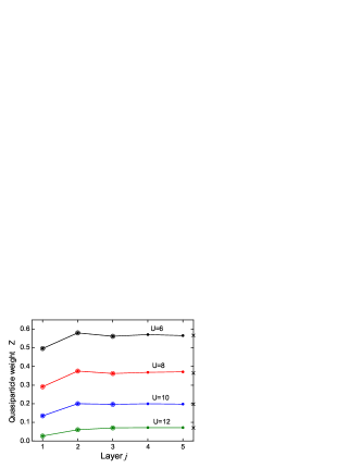
Figure 1: (color online) Quasiparticle weight $Z$ of semi-infinite Hubbard model for simple cubic lattice in the (001) orientation as a function of layer index $j$. Temperature $T=0.02$. Solid dots and open circles are results with $N=5$ and $N=3$ embedded layers, respectively. Crosses on the vertical axis indicate the bulk $Z$ corresponding to four values of $U$. Lines are drawn as a guide to the eye.

In Fig. 1 we show the calculated quasiparticle weight $Z$ of the semi-infinite Hubbard model at $T=0.02$ in the metallic range $U<U_{c}$ as a function of layer index $j$, where the outermost layer corresponds to $j=1$. The hopping integral is taken to be $t=1$ and defines the energy scale. The crosses on the vertical axis indicate the $Z$ values of the bulk metal determined by a separate bulk DMFT calculation. The embedding potential acts on layer $N$ on the right edge of the surface region. Solid dots and open circles provide the results obtained for $N=5$ and $N=3$ embedded layers, respectively. The excellent agreement between the two sets of calculations demonstrates that the embedding potential represents correctly the one-electron as well as many-body properties of the semi-infinite substrate. Moreover, it is evident that one needs only a few embedded layers to simulate the semi-infinite system. Although the latter point is not crucial for single-band model systems, for the calculation of realistic multi-orbital materials the embedding treatment yields a substantial reduction of computer time compared with slab calculations in which at least $\sim$10 layers must be explicitly taken into consideration.

As can be seen in Fig. 1, the calculated $Z$ exhibits an oscillatory behavior near the surface which follows from the Friedel oscillations of the layer-dependent density of states. In the first layer, $Z$ is smaller than the bulk value, implying that electrons at the surface are more strongly correlated than in the bulk. As discussed by Potthoff and NoltingPotthoff:99 and Liebsch,Liebsch:03 this is essentially a one-electron effect arising from the layer dependence of the one-electron DOS of the cubic tight-binding Hamiltonian.Kalkstein:71 Because of the loss of nearest-neighbor sites, the effective band width in the first layer is reduced, so that Coulomb correlations at the surface are enhanced.

Next, we study the interface between two semi-infinite Hubbard models. We consider a uniform system with regard to the transfer integrals, i.e., $t^{x}_{j}=t^{y}_{j}=t^{z}_{jk}=t=1$. In the left half-space, we choose the Coulomb energy as $U_{L}=6$ to represent a good metal with a relatively large quasiparticle weight, while we take a variable, larger Coulomb energy $U_{R}$ in the half-space on the right. Furthermore, by choosing $\epsilon_{j}$ as $-U_{L}/2$ and $-U_{R}/2$ in the left and right half-spaces, respectively, and by setting the chemical potential as $\mu=0$, all layers are half-filled. The same model was recently investigated by Helmes et al.Helmes:08 who used the NRG method as impurity solver. These authors focused on the critical range for $U_{R}\sim U_{c}$ and discussed the scaling behavior of the metallic penetration depth into the Mott insulator. To reduce finite-size effects, a relatively thick slab consisting of $\sim$60 layers was used to simulate the interface. Also, to avoid numerical difficulties stemming from the energy discretization the van Hove singularity of the two-dimensional layer DOS was cut off at a finite value.

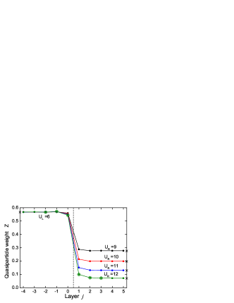
Figure 2: (color online) Quasiparticle weight $Z$ at the interface between two semi-infinite Hubbard models for simple cubic lattice in (001) orientation as a function of layer index $j$. The boundary between the two metals is marked by a dashed line. Temperature $T=0.02$. Solid dots and open circles show results with $N=10$ and $N=6$ embedded layers, respectively. Crosses on the vertical axis indicate bulk $Z$ values. Lines are drawn as a guide to the eye.

Figure 2 shows the calculated quasiparticle weight $Z$ in the metallic range $U_{R}<U_{c}$ at $T=0.02$ as a function of layer index $j$, which is measured here relative to the boundary layer of the left-hand side metal. To describe the deviation of the electronic structure from that in bulk metal, we incorporate in the embedded region $N=10$ layers (solid dots), of which the left (right) five layers possess Coulomb energy $U_{L}$ ($U_{R}$). For comparison, we also show for $U_{R}=12$ (open circles) the result obtained with only $N=6$ embedded layers. The excellent agreement between the two sets of calculations corroborates again the efficiency of the embedding method to treat semi-infinite substrates.

The quasiparticle weight $Z$ of the surface layer of the good metal on the left-hand side is seen to be reduced whereas at the surface of the poor metal on the right-hand side of the boundary plane it is enhanced. Evidently, the good or bad metallic character of one metal spills over into the neighboring metal. In contrast to the case of the semi-infinite surface discussed above, this is a genuine many-body effect, since the one-electron DOS is layer-independent if the Coulomb interaction is switched off. The deviation of $Z$ from the bulk value in poor metal on the right decreases with the distance from the boundary plane, which is in accord with the work of Helmes et al.Helmes:08 On the left of the boundary plane, $Z$ is seen to be weakly modified with respect to the bulk value only in the first two layers. Thus, as a result of better electronic screening in the good metal, $Z$ approaches the bulk value more rapidly than in the poor metal. Essentially, one needs to incorporate only one or two layers in the embedded region to describe the interface properties of the good metal on the left-hand side.

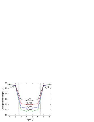
Figure 3: (color online) Quasiparticle weight $Z$ of the heterostructure consisting of a 4-layer film ($j=3\ldots 6$) sandwiched between two semi-infinite Hubbard models for simple cubic lattice in the (001) orientation. Crosses on the vertical axes indicate bulk $Z$ values for the left and right substrates. Temperature $T=0.02$. Lines are drawn as a guide to the eye.

As the third model system, we study a junction in which a finite number of strongly correlated-electron layers are sandwiched between two weakly correlated metals. We adopt again a uniform model with respect to transfer integrals, i.e., $t^{x}_{j}=t^{y}_{j}=t^{z}_{jk}=t=1$ for all layers. We assign a non-zero but moderate Coulomb energy $U_{L,R}=6$ to both metal substrates, whereas in the central film we choose a larger Coulomb energy $U_{m}$. In Fig. 3 we show the calculated quasiparticle weight $Z$ for a 4-layer film as a function of layer index $j$ in the metallic range $U_{m}<U_{c}$. The calculation was carried out using $N=8$ embedded layers, which comprise the central 4-layer film and the two outermost layers of metal substrates on both sides. Interestingly, in this thin film $Z$ is very close to that of the boundary layers of the semi-infinite metal with $U=U_{R}$ shown in Fig. 2. This rapid convergence of $Z$ with increasing film thickness may arise partly from the peculiarity of the present model in which the one-electron DOS is layer-independent. Thus, there appear no finite-size effects such as energy-level discretization in the one-electron spectrum at the junction.

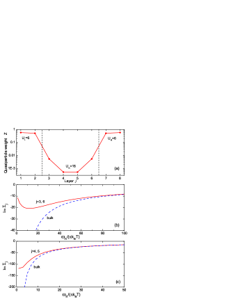
Figure 4: (color online) (a) Quasiparticle weight $Z$ of a 4-layer film with $U_{m}=16$ sandwiched between two metals with $U_{L,R}=6$ as a function of layer index $j$. Lines are drawn as a guide to the eye. (b) and (c) Imaginary part of the impurity self-energy of boundary layers ($j=3,\ 6$) and inner layers ($j=4,\ 5$) of the thin film as a function of Matsubara frequency for $U_{m}=16$ (red solid line). The corresponding bulk self-energy at the same Coulomb energy is shown by the blue dashed line.

We finally consider a metal/insulator/metal junction. Figure 4(a) shows the quasiparticle weight $Z$ of a 4-layer film with $U_{m}=16>U_{c}$ sandwiched between two metals with $U_{L,R}=6$ at temperature $T=0.02$. As discussed by Helmes et al.,Helmes:08 the metallic states decay within the insulating layers, so that $Z$ becomes finite in the film. In agreement with these NRG results we find that this penetration depth within the Mott gap is extremely short. To demonstrate this more clearly, we plot in Figs. 4(b) and (c) the imaginary part of the layer-dependent Coulomb self-energy $\Sigma_{j}(i\omega_{n})$ for the outer and inner layers of the film, respectively, as a function of Matsubara frequency. For comparison, we also show the imaginary part of the impurity self-energy in the bulk simple-cubic crystal with $U=16$. Whereas the bulk self-energy diverges as $\omega_{n}\rightarrow 0$ at this Coulomb energy, the film self-energy tends to a finite value because of its contact to the neighboring metal layers. At the film surface, the finite value is about $-10$, indicating bad metallic behavior with a rather short electron lifetime and a very small quasi-particle weight $Z\approx 0.005$. In the second layer, the limiting value of the self-energy at low $\omega_{n}$ is more than one order of magnitude larger than at the surface, implying correspondingly shorter electronic lifetime and lower quasi-particle weight $Z$. Thus, apart from a weak exponential bad-metallic tail, the Mott gap of the insulating film is virtually impenetrable.

Electron transport through correlated-electron systems such as oxide heterostructures and molecules is emerging as an active field of theoretical studies.Ferretti:05 ; Okamoto:08 ; Thygesen:08 To our knowledge, previous studies considered only non-interacting metal leads connected to a central region with Coulomb interactions. It would be interesting to extend the transport theory to the case of interacting metal leads as those shown in Figs. 3 and 4.

IV Summary

We have presented an efficient embedding scheme for performing DMFT calculations for inhomogeneous layered systems such as semi-infinite surfaces and heterostructures. In contrast to previous embedding theories based on tight-binding basis functions, the embedding potential introduced here is determined from a separate DMFT calculation for the bulk substrate materials. It therefore incorporates not only the one-electron properties but also the many-body effects of the semi-infinite systems. The interface region in which local Coulomb interactions are treated self-consistently via the layer-coupled DMFT also includes the first few layers of the actual substrates. As examples, we have presented numerical results for several surfaces and interfaces of the single-band Hubbard model. These results demonstrate that the represention of the semi-infinite correlated substrates in terms of complex energy-dependent embedding potentials greatly reduces the numerical effort since only a small number of layers needs to be explicitly included in the layer-coupled DMFT equation. Thus, the study of neutral as well as charged heterostructures involving realistic strongly correlated multi-band materials becomes feasible.

- (1) E. Dagotto, Science 318, 1076 (2007).
- (2) R. Matzdorf, Z. Fang, Ismail, J. Zhang, T. Kimura, Y. Tokura, K. Terakura, and E. W. Plummer, Science 289, 746 (2000).
- (3) K. Maiti, D. D. Sarma, M. J. Rozenberg, I. H. Inoue, H. Makino, O. Goto, M. Pedio, and R. Cimino, Europhys. Lett. 55, 246 (2001).
- (4) A. Sekiyama, H. Fujiwara, S. Imada, S. Suga, H. Eisaki, S. I. Uchida, K. Takegahara, H. Harima, Y. Saitoh, I. A. Nekrasov, G. Keller, D. E. Kondakov, A. V. Kozhevnikov, Th. Pruschke, K. Held, D. Vollhardt, and V. I. Anisimov, Phys. Rev. Lett. 93, 156402 (2004).
- (5) A. Ohtomo, D. A. Muller, J. L. Grazul, and H. Y. Hwang, Nature (London) 419, 378 (2002).
- (6) M. Takizawa, H. Wadati, K. Tanaka, M. Hashimoto, T. Yoshida, A. Fujimori, A. Chikamatsu, H. Kumigashira, M. Oshima, K. Shibuya, T. Mihara, T. Ohnishi, M. Lippmaa, M. Kawasaki, H. Koinuma, S. Okamoto, and A. J. Millis, Phys. Rev. Lett. 97, 057601 (2006).
- (7) L. F. Kourkoutis, Y. Hotta, T. Susaki, H. Y. Hwang, and D. A. Muller, Phys. Rev. Lett. 97, 256803 (2006).
- (8) K. Maekawa, M. Takizawa, H. Wadati, T. Yoshida, A. Fujimori, H. Kumigashira, M. Oshima, Y. Muraoka, Y. Nagao, and Z. Hiroi, Phys. Rev. B 76, 115121 (2007).
- (9) H. Wadati, Y. Hotta, A. Fujimori, T. Susaki, H. Y. Hwang, Y. Takata, K. Horiba, M. Matsunami, S. Shin, M. Yabashi, K. Tamasaku, Y. Nishino, and T. Ishikawa, Phys. Rev. B 77, 045122 (2008).
- (10) A. Georges, G. Kotliar, W. Krauth, and M. J. Rozenberg, Rev. Mod. Phys. 68, 13 (1996).
- (11) For recent reviews, see: K. Held, Adv. in Physics, 56, 829 (2007); G. Kotliar, S. Y. Savrasov, K. Haule, V. S. Oudovenko, O. Parcollet, and C. A. Marianetti, Rev. Mod. Phys. 78, 865 (2006).
- (12) M. Potthoff and W. Nolting, Phys. Rev. B 59, 2549 (1999); Phys. Rev. B 60, 7834 (1999).
- (13) See also: M. Potthoff, Phys. Rev. B 64, 165114 (2001); S. Schwieger, M. Potthoff and W. Nolting, Phys. Rev. B 67, 165408 (2003).
- (14) A. Liebsch, Phys. Rev. Lett. 90, 096401 (2003); Europhys. J. B 32, 477 (2003).
- (15) R. W. Helmes, T. A. Costi, and A. Rosch, Phys. Rev. Lett 101, 066802 (2008).
- (16) S. Okamoto and A. J. Millis, Phys. Rev. B 70, 075101 (2004); Phys. Rev. B 70, 241104 (R) (2004).
- (17) S. Okamoto and A. J. Millis, Phys. Rev. B 72, 235108 (2005).
- (18) S. S. Kancharla and E. Dagotto, Phys. Rev. B 74, 195327 (2006).
- (19) A. Rüegg, S. Pilgram, and M. Sigrist, Phys. Rev. B 75, 195117 (2007).
- (20) T. Oka and N. Nagaosa, Phys. Rev. Lett. 95, 266403 (2005).
- (21) W.-Ch. Lee and A. H. MacDonald, Phys. Rev. B 74, 075106 (2006); Phys. Rev. B 76, 075339 (2007).
- (22) I. González, S. Okamoto, S. Yunoki, A. Moreo, and E. Dagotto, arXiv:0801.2174 (unpublished).
- (23) A. Ferretti, A. Calzolari, R. D. Felice, F. Manghi, M. J. Caldas, M. B. Nardelli, and E. Molinari, Phys. Rev. Lett. 94, 116802 (2005).
- (24) S. Okamoto, Phys. Rev. Lett. 101, 116807 (2008).
- (25) L. Chen and J. K. Freericks, Phys. Rev. B 75, 125114 (2007); see also: J. K. Freericks, Phys. Rev. B 70, 195342 (2004); J. K. Freericks, V. Zlatić, and A. M. Shvaika, Phys. Rev. B 75, 035133 (2007).
- (26) J. E. Inglesfield, Comput. Phys. Commun. 137, 89 (2001).
- (27) G. A. Baraff and M. Schlüter, J. Phys. C 19, 4383 (1986).
- (28) C. Pisani, R. Dovesi, and P. Carosso, Phys. Rev. B 20, 5345 (1979).
- (29) S. Datta, Electronic Transport in Mesoscopic Systems, (Cambridge University Press, Cambridge U.K., 1995).
- (30) K. S. Thygesen and A. Rubio, Phys. Rev. B 77, 115333 (2008).
- (31) N. Marzari and D. Vanderbilt, Phys. Rev. B 56, 12847 (1997).
- (32) J. E. Hirsch and R. M. Fye, Phys. Rev. Lett. 56, 2521 (1986).
- (33) A. Georges and W. Krauth, Phys. Rev. Lett. 69, 1240 (1992).
- (34) M. Caffarel and W. Krauth, Phys. Rev. Lett. 72, 1545 (1994).
- (35) R. Bulla, T. A. Costi, and T. Pruschke, Rev. Mod. Phys. 80, 395 (2008).
- (36) D. Kalkstein and P. Soven, Surf. Sci. 26, 85 (1971).
- (37) C. A. Perroni, H. Ishida, and A. Liebsch, Phys. Rev. B 75, 045125 (2007).