High order resolution of the Maxwell-Fokker-Planck-Landau model intended for ICF applications

Abstract.

A high order, deterministic direct numerical method is proposed for the nonrelativistic $2D_{\bf x}\times 3D_{\bf v}$ Vlasov-Maxwell system, coupled with Fokker-Planck-Landau type operators. Such a system is devoted to the modelling of electronic transport and energy deposition in the general frame of Inertial Confinement Fusion applications. It describes the kinetics of plasma physics in the nonlocal thermodynamic equilibrium regime. Strong numerical constraints lead us to develop specific methods and approaches for validation, that might be used in other fields where couplings between equations, multiscale physics, and high dimensionality are involved. Parallelisation (MPI communication standard) and fast algorithms such as the multigrid method are employed, that make this direct approach be computationally affordable for simulations of hundreds of picoseconds, when dealing with configurations that present five dimensions in phase space.

Keywords. High order numerical scheme, Fokker-Planck-Landau, NLTE regime, ICF, Magnetic field, Electronic transport, Energy deposition.

AMS subject classifications.

1. Introduction

In the context of the interaction of intense, short laser pulses with solid targets [29], Inertial Confinement Fusion (ICF) schemes [3, 33], the energy transport is an important issue. In this latter field of applications (ICF), it determines the efficiency of plasma heating and the possibility to achieve the fusion conditions. The appropriate scales under consideration here are about one hundred of micrometers for the typical spatial sizes, and one hundred of picoseconds for the time scales.

Several key features should be accounted for. First of all, in typical ICF configurations, a significant amount of energetic electrons have a large mean free path, exceeding the characteristic gradient length of the temperature and the density: the particles motion exhibits nonlocal features.

A wide range of collisional regimes should be dealt with to describe the propagation and the deposit of energetic electrons from the underdense corona of the target to its dense and compressed core.

The collisions are important even if the beam particles themselves are collisionless [3] : these particles, when propagating in a plasma, trigger a return current that neutralizes the incident current. This return current is determined by collisions of thermal, background electrons. The structure of the generated electron distribution function is then often anisotropic, with a strongly intercorrelated two population structure. For nonrelativistic laser intensities, smaller than $10^{18}\,\mbox{W}\,\mbox{cm}^{-2}$, a small angle description for collisions between the two populations is well-suited, leading to the classical Fokker-Planck-Landau collision model. The Coulomb potential involves a large amount of collisions with small energy exchanges between particles, so that the Landau form of the Fokker-Planck operator is required here. Such a configuration with two counterstreaming beams typically leads to the developement of microscopic instabilities that can modify strongly the beam propagation. We refer to the two-stream and filamentation instabilities, where the wave vector of the perturbation is respectively parallel and perpendicular to the incident beam [7, 8]. A self-consistent description of electromagnetic fields is then required to describe the plasma behaviour and associated instabilities. Furthermore in the process of plasma heating, strong magnetic fields are generated at intensity that can reach a MegaGauss scale and may affect the energy transport [6, 21, 23]. The sources of magnetic field generation include on the one hand the effects of the rotational part of the electronic pressure which is a cross gradient $\nabla T\times\nabla n$ effect, and on the other hand the exponential growth of perturbations of anisotropic distribution functions (Weibel instability). Some electromagnetic processes can be strongly coupled with nonlocal effects.

The plasma model studied in this paper is based on the nonrelativistic Vlasov-Maxwell equations, coupled with Fokker-Planck-Landau collision operators. It gathers the listed requirements at laser intensities which are relevant for ICF. At higher laser intensities, a relativistic treatment should be considered [3, 36], and collision operators with large energy exchanges are required if secondary fast electron production proves to be non-negligible, paticularly with dense plasmas.

There are several numerical methods that treat the Vlasov-Maxwell model together with Fokker-Planck-Landau type operators. Among them, the Particle-In-Cell (PIC) methods provide satisfying results only in a limited range of collisional regimes. Moreover, they suffer from the “finite grid instability”, that leads to numerical heating. Also the statistical noise and the low resolution of the electron distribution function by PIC solvers lead generally to an inaccurate treatment of collisions, particularly when dealing with low temperature and high density plasmas. Another approach consists in the expansion of the distribution function in Legendre polynomials, retaining the lowest order terms. However, with this approach, a strong anisotropy of the distribution function cannot be treated [3, 22, 1]. Both of these methods are well-suited in particular regimes but fail at modelling more complicated situations where a collisionless anisotropic fast electron population is coupled to a collision dominated thermal population. To overcome these difficulties, a spherical harmonic expansion has been proposed, that proves to be efficient [3]. Here we propose a different approach which consists in approximating the full model by a direct deterministic numerical method. It discretizes directly the initial set of equations and enables to preserve, at a discrete level, the physical invariants of the model (positivity of the distribution function, total mass and energy, entropy decreasing behaviour, etc). Many deterministic schemes of this type have already been considered for homogeneous Fokker-Planck type operators [14, 9, 10, 27]. The nonhomogeneous case, that includes the transport part (see [20] for a comparison between Eulerian Vlasov solvers), involves a large computational complexity that can only be reduced with fast algorithms. Multipole expansion [26] and multigrid [10] techniques, as well as fast spectral methods [27, 19], have been applied to the Landau equation. For computational complexity constraints, very few results on the accuracy of these methods are known in the nonhomogeneous case [12, 19], particularly when the coupling with magnetic fields is considered.

Our starting point for the transport part discretization is a second order finite volume scheme introduced in [12]. Its main feature is that it preserves exactly the discrete energy, if slope limiters are not active. We intoduce additional dissipation on these limiters in order to successfully address the two-stream instability test case. We will underline the important role of the limitation procedure for the accuracy, on the second order scheme. This scheme is compared in this test case with a fourth order MUSCL scheme [35], with a limitation ensuring the positivity of the distribution function [5]. A similar approach, with the introduction of a fourth order scheme for transport to avoid numerical heating, has already been proposed in the context of PIC solvers [32]. The discretization of the Maxwell equations is performed with a Crank-Nicholson method, allowing to have time steps of the order of the collision time. It is designed to preserve the discrete total electromagnetic energy, which is a very important numerical constraint when considering the coupling of Vlasov and Maxwell equations for applications aiming at capturing an accurate energy deposition. We use for the Landau operator a fast multigrid technique that proves to be accurate in a wide range of collisional regimes. Moreover, the use of domain decomposition techniques and distributed memory MPI standard on the space domain leads to affordable computational cost, allowing to treat time dependent $2D_{\bf x}\times 3D_{\bf v}$ problems. As for the Lorentz electron-ion collision operator, we insist on discrete symmetry properties that are important when coupling to the Maxwell equations.

Finally, we propose to validate the numerical method on several physical test cases.

The paper is organized as follows. First, we present the model and its properties, then we discuss the numerical schemes for the transport part, their properties, and propose several numerical tests. Then the discretization for the collision operators is treated and we finally present physical test cases $1D_{x}\times 3D_{\bf v}$ and $2D_{\bf x}\times 3D_{\bf v}$ that show the accuracy of the present algorithm.

2. Kinetic model

Two particle species are considered: ions which are supposed to be fixed (assuming an electron-ion mass ratio $m_{e}/m_{i}\ll 1$), and electrons for which the evolution is described by a distribution function $f_{e}(t,{\bf x},{\bf v})$ where for the more general case $({\bf x},{\bf v})\,\in\,\Omega\times\mathbb{R}^{3}$, with $\Omega\subset\mathbb{R}^{3}$. The nonrelativistic Vlasov equation with Fokker-Planck-Landau (FPL) collision operator is given by

(1) $$\frac{\partial f_{e}}{\partial t}\,+\,\nabla_{{\bf x}}\cdot\left({\bf v}\,f_{e}\right)\,+\,\frac{q_{e}}{m_{e}}\,\nabla_{{\bf v}}\cdot\left(({\bf E}\,+\,{\bf v}\times{\bf B})\,f_{e}\right)\,=\,C_{e,e}(f_{e},f_{e})\,+\,C_{e,i}(f_{e}),$$

where $q_{e}=-e$ is the charge of an electron and $m_{e}$ is the mass of an electron. On the one hand, electromagnetic fields $({\bf E},{\bf B})$ are given by the classical Maxwell system

(2) $$\left\{\begin{array}[]{l}\displaystyle{\frac{\partial{\bf E}}{\partial t}\,-\,c^{2}\,\nabla_{\bf x}\times{\bf B}\,=\,-\frac{\bf J}{\epsilon_{0}}},\\ \\ \displaystyle{\frac{\partial{\bf B}}{\partial t}+\nabla_{\bf x}\times{\bf E}\,=\,0,}\end{array}\right.$$

where $\epsilon_{0}$ represents the permittivity of vacuum, $c$ is the speed of light. The electric current is given by

$${\bf J}(t,{\bf x})\,=\,q_{e}\int_{\mathbb{R}^{3}}f_{e}(t,{\bf x},{\bf v})\,{\bf v\,dv}.$$

Moreover, Maxwell system’s is supplemented by Gauss law’s

(3) $$\nabla_{\bf x}\cdot{\bf E}\,=\,\frac{\rho}{\epsilon_{0}},\quad\nabla_{\bf x}\cdot{\bf B}\,=\,0,$$

where $\rho$ is the charge density:

$$\rho\,=\,q_{e}\,(n_{e}-{n_{o}})\,=\,q_{e}\,\left(\int_{\mathbb{R}^{3}}f_{e}(t,{\bf x},{\bf v})\,{\bf dv}\,-\,{n_{0}}\right),$$

and ${n_{0}}/{Z}$ is the initial ion density.

On the other hand in (1), the right hand side represents collisions between particles, which only act on the velocity variable, so we drop the ${\bf x}$ variable. The operator $C_{e,e}(f_{e},f_{e})$ stands for the electron-electron collision operator whereas $C_{e,i}(f_{e})$ is the electron-ion collision operator

(4) $$C_{e,e}(f_{e},f_{e})\,=\,\frac{e^{4}\,\ln\Lambda}{8\,\pi\,\epsilon_{0}^{2}\,m_{e}^{2}}\,\nabla_{\bf v}\cdot\left(\int_{\mathbb{R}^{3}}\Phi({\bf v}-{\bf v}^{\prime})\left[f_{e}({\bf v}^{\prime})\nabla_{\bf v}f_{e}({\bf v})-f_{e}({\bf v})\nabla_{\bf v^{\prime}}f_{e}({\bf v}^{\prime})\right]{\bf dv^{\prime}}\right),$$

whereas $C_{e,i}(f_{e})$ is the electron-ion collision operator

(5) $$C_{e,i}(f_{e})\,=\,\frac{Z\,n_{0}\,e^{4}\ln\Lambda}{8\,\pi\,\epsilon_{0}^{2}\,m_{e}^{2}}\,\nabla_{\bf v}\cdot\left[\Phi({\bf v})\nabla_{\bf v}f_{e}({\bf v})\right].$$

where $\ln\Lambda$ is the Coulomb logarithm, which is supposed to be constant over the domain and $\Phi({\bf u})$ is an operator acting on the relative velocity ${\bf u}$

(6) $$\Phi({\bf u})=\frac{\|{\bf u}\|^{2}\,{\rm Id}\,-\,{\bf u}\otimes{\bf u}}{\|{\bf u}\|^{3}}.$$

As we assume ions to be fixed, the FPL operator can then be simplified for electron-ion collisions [12], and reduced to the Lorentz approximation. We refer to [2] for a physical derivation.

In this model, the Vlasov equation stands for the invariance of the distribution function along the particles trajectories affected by the electric and magnetic fields ${\bf E}$ and ${\bf B}$. The Vlasov equation representing the left-hand side in (1) is written in a conservative form, but it can also be written in an equivalent non-conservative form, while Maxwell equations (2)-(3) provide with a complete self-consistent description of electromagnetic fields. The coupling between both is performed via the Lorentz force term ${\bf E}\,+\,{\bf v}\times{\bf B}$ in the Vlasov equation, and the current source terms in Maxwell equations. Furthermore, the FPL operator is used to describe elastic, binary collisions between charged particles, with the long-range Coulomb interaction potential. Classical but important properties of the system (1)-(3) together with operators (4) and (5), are briefly recalled. For detailed proofs, we refer to [12, 13].

2.1. Transport equation under electromagnetic fields

Let us neglect in this section the collision operators. The Vlasov-Maxwell system (1)-(3) with a zero right-hand side is strictly equivalent to (1)-(2) provided Gauss’s laws (3) are initially satisfied. This gives a compatibility condition at initial time.
The mass and momentum are preserved with respect to time for the Vlasov-Maxwell system, i.e. system (1)-(2) without collision operators

$$\frac{d}{dt}\int_{\mathbb{R}^{3}\times\mathbb{R}^{3}}f_{e}(t,{\bf x},{\bf v})\left(\begin{array}[]{l}1\\ {\bf v}\end{array}\right){\bf dx\,dv}\,=\,0,\,\,t\geq 0.$$

Moreover, conservation of energy can be proved for the Vlasov-Maxwell system by multiplying equation (1) by $m_{e}\,\|{\bf v}\|^{2}/2$ and integrating it in the velocity space. It gives after an integration by parts

$$\frac{1}{2}\,\frac{d}{dt}\int_{\mathbb{R}^{3}}\left\{\epsilon_{0}\,\|{\bf E}(t,{\bf x})\|^{2}\,+\,\frac{1}{\mu_{0}}\|{\bf B}(t,{\bf x})\|^{2}\,+\,\left[\int_{\mathbb{R}^{3}}m_{e}\|{\bf v}\|^{2}f_{e}(t,{\bf x},{\bf v}){\bf dv}\right]\,\right\}\,{\bf dx}\,=\,0,\,\,t\geq 0,$$

with $c^{2}\,\epsilon_{0}\,\mu_{0}\,=\,1$. The Vlasov-Maxwell system also conserves the kinetic entropy

$$\frac{d}{dt}H(t)\,=\,\frac{d}{dt}\int_{\mathbb{R}^{3}\times\mathbb{R}^{3}}f_{e}(t,{\bf x},{\bf v})\log(f_{e}(t,{\bf x},{\bf v}))\,{\bf dx\,dv}\,=\,0,\,\,t\geq 0.$$

2.2. Collision operators

The FPL operator is used to describe binary elastic collisions between electrons. Its algebraic structure is similar to the Boltzmann operator, in that it satisfies the conservation of mass, momentum and energy

$$\int_{\mathbb{R}^{3}}C_{e,e}(f_{e},f_{e})({\bf v})\left(\begin{array}[]{c}1\\ {\bf v}\\ \|{\bf v}\|^{2}\end{array}\right){\bf dv}\,=\,0,\,\,t\geq 0.$$

Moreover, the entropy is decreasing with respect to time

$$\frac{dH}{dt}(t)=\frac{d}{dt}\int_{\mathbb{R}^{3}}f_{e}({\bf v},t)\,\log(f_{e}({\bf v},t)){\bf dv}\,\leq\,0,\,\,t\geq 0.$$

The equilibrium states of the FPL operator, i.e. the set of distribution functions in the kernel of $C_{e,e}(f_{e},f_{e})$, are given by the Maxwellian distribution functions

$${\mathcal{M}}_{n_{e},{\bf u_{e}},T_{e}}({\bf v})\,=\,n_{e}\left(\frac{m_{e}}{2\,\pi\,T_{e}}\right)^{3/2}\exp\left(-m_{e}\,\frac{\|{\bf v}-{\bf u_{e}}\|^{2}}{2\,T_{e}}\right),$$

where $n_{e}$ is the density, ${\bf u_{e}}$ is the mean velocity and $T_{e}$ is the temperature, defined as

$$\left\{\begin{array}[]{l}\displaystyle{n_{e}\,=\,\int_{\mathbb{R}^{3}}f_{e}({\bf v}){\bf dv},}\\ \\ \displaystyle{{\bf u_{e}}\,=\,\frac{1}{n_{e}}\int_{\mathbb{R}^{3}}f_{e}({\bf v}){\bf v}{\bf dv},}\\ \\ \displaystyle{T_{e}\,=\,\frac{m_{e}}{3\,n_{e}}\int_{\mathbb{R}^{3}}f_{e}({\bf v})\|{\bf v}-{\bf u_{e}}\|^{2}{\bf dv}.}\end{array}\right.$$

On the other hand, the operator (5), modelling collisions between electrons and ions, is a Lorentz operator. It satisfies the conservation of mass and energy

$$\int_{\mathbb{R}^{3}}C_{e,i}(f_{e})({\bf v})\left(\begin{array}[]{c}1\\ \|{\bf v}-{\bf u_{e}}\|^{2}\end{array}\right)\,{\bf dv}\,=\,0.$$

Moreover, the equilibrium states for this operator are given by the set of isotropic functions:

$${\rm Ker}\left(C_{e,i}\right)\,=\,\left\{\,f_{e}\in L^{1}\left((1+\|{\bf v}\|^{2}){\bf dv}\right),\quad f_{e}({\bf v})\,=\,\phi(z),\,\,\,z\,=\,\|{\bf v}-{\bf u_{e}}\|^{2}\,\right\}.$$

Finally, each convex function $\psi$ of $f_{e}$ is an entropy for $C_{e,i}(f_{e})$,

$$\frac{d}{dt}\int_{\mathbb{R}^{3}}\psi(f_{e})\,{\bf dv}\,\leq\,0,\,\,t\geq 0.$$

In addition to these properties, we present a symmetry property. This property may have some importance, in particular in presence of magnetic fields. In that case, any break of symmetry due to an inadequate discretization method could lead to generation of an artificial magnetic field, via the current source terms, when coupling with the Maxwell equations.

Proposition 2.1.

If $f_{e}$ has the following symmetry property with respect to the direction $k$ at time $t_{0}$

(7) $$f_{e}(t_{0},{\bf v})\,\,=\,\,f_{e}(t_{0},{\bf v}^{k}),$$

with components for

$${\bf v}^{k}_{i}\,=\,\left\{\begin{array}[]{ll}+{\bf v}_{i}&\textrm{ if }i\neq k,\\ -{\bf v}_{i}&\textrm{ if }i=k.\end{array}\right.$$

Then, this symmetry property is preserved with respect to time.

3. Numerical scheme for transport

We present a finite volume approximation for the Vlasov-Maxwell system (1)-(2) without collision operators. Indeed, it is crucial to approximate accurately the transport part of the system to asses the collective behaviour of the plasma, that occurs typically at a shorter scale than the collision processes. We introduce a uniform $1D$ space discretization $(x_{i+1/2})_{i\in I}$, $I\subset\mathbb{N}$, of the interval $(0,L_{1})$, in the direction denoted by index $1$. The associated space variable is denoted by $x_{1}$. We define the control volumes $C_{i,{\bf j}}=(x_{i-1/2},x_{i+1/2})\times({\bf v}_{\bf j-1/2},{\bf v}_{\bf j+1/2})$, the size of a control volume in one direction in space $\Delta x$ and velocity $\Delta v$.

The velocity variable ${\bf v}={}^{t}(v_{1},v_{2},v_{3})$ is discretized on the grid ${\bf v}_{\bf j}\,=\,{\bf j}\,\Delta v\,=\,{}^{t}(v_{j_{1}},v_{j_{2}},v_{j_{3}})$ with ${\bf j}={}^{t}(j_{1},j_{2},j_{3})\in\mathbb{Z}^{3}$. Moreover we note ${\bf v}_{\bf j+1/2}\,=\,{}^{t}(j_{1}+1/2,j_{2}+1/2,j_{3}+1/2)\,\Delta v$. Finally, the time discretization is defined as $t^{n}\,=\,n\Delta t$, with $n\in\mathbb{N}$.

Let $f_{i,{\bf j}}^{n}$ be an average approximation of the distribution function on the control volume $C_{i,{\bf j}}$ at time $t^{n}$, that is

$$f_{i,{\bf j}}^{n}\,\simeq\,\frac{1}{\Delta x\,\Delta v^{3}}\int_{C_{i,{\bf j}}}f(t^{n},x,{\bf v})dx\,{\bf dv}.$$

Moreover since the discretization is presented in a simple $1D_{x}$ space geometry, the electromagnetic field has the follownig structure: ${\bf E}={}^{t}(E_{1}(t,x_{1})),E_{2}(t,x_{1}),0)$, ${\bf B}={}^{t}(0,0,B_{3}(t,x_{1}))$. Hence ${}^{t}(E_{1,i}^{n},E_{2,i}^{n})$ is an approximation of the electric field ${}^{t}(E_{1},E_{2})$ whereas $B_{3,i}^{n}$ represents an approximation of the magnetic field $B_{3}$ in the control volume $(x_{i-1/2},x_{i+1/2})$ at time $t^{n}$.

3.1. Second order approximation of a one dimensional transport equation

For the sake of simplicity, we focus on the discretization of a $1D$ transport equation; the extension to higher dimensions is straightforward on a grid, without requiring time splitting techniques between transport terms. In this section, the index $1$ is dropped both on space and velocity directions, for this simple $1D_{x}$ geometry.

Let us consider the following equation for $t\geq 0$ and $x\in(0,L)$,

(8) $$\frac{\partial f}{\partial t}\,+\,v\,\frac{\partial f}{\partial x}\,=\,0\ ,$$

where the velocity $v>0$ is given. By symmetry it is possible to recover the case when $v$ is negative. In the following we skip the velocity variable dependency of the distribution function. Using a time explicit Euler scheme and integrating the $1D$ Vlasov equation on a control volume $(x_{i-1/2},x_{i+1/2})$, it yields

(9) $$f_{i}^{n+1}\,=\,f_{i}^{n}-\frac{\Delta t}{\Delta x}\,\left[\mathcal{F}_{i+1/2}^{n}-\mathcal{F}_{i-1/2}^{n}\right],$$

where $\mathcal{F}_{i+1/2}^{n}$ represents an approximation of the flux $v\,f(t^{n},x_{i+1/2})$ at the interface $x_{i+1/2}$.

The next step consists in approximating the fluxes and to reconstruct the distribution function. To this aim, we approximate the distribution function $f(t^{n},x)$ by $f_{h}(x)$ using a second order accurate approximation of the distribution function on the interval $[x_{i-1/2},x_{i+1/2})$, with a reconstruction technique by primitive [12]

(10) $$f_{h}(x)=f_{i}^{n}\,+\,\epsilon_{i}^{+}\,\frac{(x-x_{i})}{\Delta x}(f_{i+1}^{n}\,-\,f_{i}^{n}).$$

We introduce the limiter

(11) $$\epsilon_{i}^{+}=\left\{\begin{array}[]{ll}0&\textrm{ if }(f_{i+1}^{n}-f_{i}^{n})\,(f_{i}^{n}-f_{i-1}^{n})\,<\,0,\\ \min\left(1,\displaystyle{\frac{2\left(\|f^{0}\|_{\infty}-f^{n}_{i}\right)}{f^{n}_{i}-f^{n}_{i+1}}}\right)&\textrm{ if }(f_{i+1}^{n}-f_{i}^{n})<0\ ,\\ \min\left(1,\displaystyle{\frac{2\,f_{i}^{n}}{f_{i+1}^{n}-f_{i}^{n}}}\right)&\textrm{ else,}\end{array}\right.$$

and set $\mathcal{F}_{i+1/2}^{n}=v\,f_{h}(x_{i+1/2})$. This type of limiter introduces a particular treatment for extrema. At this price only (dissipation at extrema), we were able to recover correctly the two-stream instabililty test case, without oscillations destroying the salient features of the distribution function structure. Another choice for the limitation consits in choosing the “Van Leer’s one parameter family of the minmod limiters” [24]

(12) $$\epsilon_{i}^{+}=\mbox{minmod}\left(b\frac{(f_{i+1}^{n}-f_{i}^{n})}{\Delta x},\frac{(f_{i+1}^{n}-f_{i-1}^{n})}{2\Delta x},b\frac{(f_{i}^{n}-f_{i-1}^{n})}{\Delta x}\right),\,$$

where

$$\mbox{minmod}(x,y,z)\equiv\mbox{max}(0,\mbox{min}(x,y,z))+\mbox{min}(0,\mbox{max}(x,y,z))\ ,\quad(x,y,z)\in\mathbb{R}{{}^{3}},$$

and $b$ is a parameter between $1$ and $2$. We will see on the two-stream instability test case the importance of the choice for limiters.
Finally, this reconstruction ensures the conservation of the average and maximum principle on $f_{h}(x)$ [12].

3.2. Fourth order transport scheme

We turn now to a higher order approximation (fourth order MUSCL TVD scheme) [35]. This scheme has also been considered in [5], in the frame of VFRoe schemes for the shallow water equations, where the authors proposed an additional limitation. Here we note that an optimized limitation procedure is possible in our case, breaking the similar treatment for both right and left increments, and taking advantage of the structure of the flux in the nonrelativistic Vlasov equation: the force term does not depend of the advection variable.

For this MUSCL scheme, we only provide here with the algorithm for the implementation of this scheme and refer to [5], [35] for the derivation procedure of this scheme.
The high order flux at the interface $x_{i+1/2}$, at time $t^{n}$ reads

(15) $$\displaystyle\mathcal{F}_{i+1/2}^{n}=\mathcal{F}\left(f_{i,r}^{n},f_{i+1,l}^{n}\right)=\left\{\begin{array}[]{c}vf_{i,r}^{n}\quad\ \ \ \mbox{if}\quad v>0\ ,\\ vf_{i+1,l}^{n}\quad\mbox{if}\quad v<0\ .\end{array}\right.$$

This numerical flux involves the reconstructed states: $\displaystyle f_{i,r}^{n}=f_{i}^{n}+(\Delta f)_{i}^{+}$ and $\displaystyle f_{i,l}^{n}=f_{i}^{n}+(\Delta f)_{i}^{-},$ where $(\Delta f)_{i}^{\pm}$ are the reconstruction increments.
An intermediate state $f_{i}^{*}$, defined by $\displaystyle\frac{1}{3}\left(f_{i,r}^{n}+f_{i}^{*}+f_{i,l}^{n}\right)=f_{i}^{n}$ si introduced. It is shown in [5] that the introduction of this intermediate state preserves, provided the CFL condition is formally divided by three, the positivity of the distribution function. Following [35] and [5], the fourth order MUSCL reconstruction reads

Algorithm of reconstruction.

Compute

$\displaystyle{\left(\Delta f\right)_{i}^{-}=-\frac{1}{6}\left(2\Delta^{*}\bar{f}_{i-1/2}+\Delta^{*}\tilde{f}_{i+1/2}\right),}$

$\displaystyle{\left(\Delta f\right)_{i}^{+}=\frac{1}{6}\left(\Delta^{*}\bar{f}_{i-1/2}+2\Delta^{*}\tilde{f}_{i+1/2}\right),}$

where

$\displaystyle{\Delta^{*}\bar{f}_{i-1/2}=\mbox{minmod}(\Delta^{*}f_{i-1/2},4\Delta^{*}f_{i+1/2}),}$

$\displaystyle{\Delta^{*}\tilde{f}_{i+1/2}=\mbox{minmod}(\Delta^{*}f_{i+1/2},4\Delta^{*}f_{i-1/2})}$

and

$\displaystyle{\Delta^{*}f_{i+1/2}=\Delta f_{i+1/2}-\frac{1}{6}\Delta^{3}\bar{f}_{i+1/2},}$

$\displaystyle{\Delta^{3}\bar{f}_{i+1/2}=\Delta\bar{f}^{a}_{i-1/2}-2\Delta\bar{f}^{b}_{i+1/2}+\Delta\bar{f}^{c}_{i+3/2},}$

with

$\displaystyle{\Delta\bar{f}^{a}_{i-1/2}=\mbox{minmod}(\Delta f_{i-1/2},2\Delta f_{i+1/2},2\Delta f_{i+3/2}),}$

$\displaystyle{\Delta\bar{f}^{b}_{i+1/2}=\mbox{minmod}(\Delta f_{i+1/2},2\Delta f_{i+3/2},2\Delta f_{i-1/2}),}$

$\displaystyle{\Delta\bar{f}^{c}_{i+3/2}=\mbox{minmod}(\Delta f_{i+3/2},2\Delta f_{i-1/2},2\Delta f_{i+1/2}),}$

with the notation $\Delta f_{i+1/2}=f_{i+1}-f_{i}$.

Reminding that the minmod limiter is given by

(21) $$\mbox{minmod}(x,y)=\left\{\begin{array}[]{ll}0,&\textrm{ if }x\,y\leq 0,\\ \\ x&\textrm{ if }|x|\,\leq|y|,\\ \\ y&\textrm{else,}\end{array}\right.$$

with $$(x,y)\in\mathbb{R}^{3}$$.

The limitation proposed in [5] is then applied.

It allows to satisfy the positivity of the reconstructed states.

Algorithm for the limitation involving the intermediate state.

Compute $(\Delta f)_{i}^{{\rm lim},\pm}$ such that

$\displaystyle{f_{i}^{n}+(\Delta f)_{i}^{{\rm lim},-}\geq 0,}$

$\displaystyle{f_{i}^{n}+(\Delta f)_{i}^{{\rm lim},+}\geq 0,}$

and

$\displaystyle{f^{*}_{i}=f_{i}^{n}-(\Delta f)_{i}^{{\rm lim},-}-(\Delta f)_{i}^{{\rm lim},+}\geq 0.}$

This limitation reads:

$\displaystyle{\left\{\begin{array}[]{l}(\Delta f)_{i}^{{\rm lim},-}\,=\,\theta\,\max\left((\Delta f)_{i}^{-},-f_{i}^{n}\right),\\ \\ (\Delta f)_{i}^{{\rm lim},+}\,=\,\theta\,\max\left((\Delta f)_{i}^{+},-f_{i}^{n}\right),\end{array}\right.}$

where

$\displaystyle{\theta\,=\,\left\{\begin{array}[]{ll}1,\quad\mbox{if}\quad\max\left((\Delta f)_{i}^{-},-f_{i}^{n}\right)\,+\,\max\left((\Delta f)_{i}^{+},-f_{i}^{n}\right)\leq 0\ ,\\ \\ \min\left(1,\frac{f_{i}^{n}}{\max\left((\Delta f)_{i}^{-},-f_{i}^{n}\right)\,+\,\max\left((\Delta f)_{i}^{+},-f_{i}^{n}\right)}\right)\quad\mbox{otherwise.}\end{array}\right.}$

3.3. Application to the Vlasov-Maxwell system.

We exactly follow the same idea to design a scheme for the full Vlasov equation in phase space $({\bf x},{\bf v})\in\Omega\times\mathbb{R}^{3}$. In addition, a centered formulation for the electromagnetic fields is chosen:

(22) $${\bf E}^{n+1/2}\,=\;\frac{1}{2}\left({\bf E}^{n+1}\,+\,{\bf E}^{n}\right)\quad\mbox{and}\quad{\bf B}^{n+1/2}\,=\,\frac{1}{2}\left({\bf B}^{n+1}+{\bf B}^{n}\right).$$

The discretization of the Maxwell equations (2)-(3) is performed via an implicit $\theta$-scheme, with $\theta=1/2$, which corresponds to the Crank-Nicholson scheme and thus preserves the total discrete energy. This discretization is presented in a simple $1D$ space geometry. The electric field ${\bf E}={}^{t}(E_{1},E_{2},0)$ and the magnetic field ${\bf B}={}^{t}(0,0,B_{3})$ are collocated data on the discrete grid. These fields are solution of the system

(23) $$\left\{\begin{array}[]{l}\displaystyle{\frac{E^{n+1}_{1,i}-E^{n}_{1,i}}{\Delta t}\,=\,-\frac{{J}_{1,i}^{n}}{\epsilon_{0}}},\\ \\ \displaystyle{\frac{E^{n+1}_{2,i}-E^{n}_{2,i}}{\Delta t}\,+\,c^{2}\,\frac{B^{n+1/2}_{3,{i+1}}-B^{n+1/2}_{3,{i-1}}}{2\Delta x}\,=\,-\frac{{J}_{2,i}^{n}}{\epsilon_{0}}},\\ \\ \displaystyle{\frac{B^{n+1}_{3,i}-B^{n}_{3,i}}{\Delta t}\,+\,\frac{E^{n+1/2}_{2,{i+1}}-E^{n+1/2}_{2,{i-1}}}{2\Delta x}\,=\,0}.\end{array}\right.$$

This scheme is well suited for the electrodynamics situations that are treated here in the test cases.
The approximation for the current in (23) ${J}_{1}^{n}$ and ${J}_{2}^{n}$ has been chosen such as

(24) $${J}_{1,i}^{n}\,=\,\sum_{{\bf j}\in\mathbb{Z}^{3}}\Delta v^{3}\,v_{j_{1}}\,f_{{i},{\bf j}}^{n}\quad\textrm{ and }\quad{J}_{2,i}^{n}\,=\,\sum_{{\bf j}\in\mathbb{Z}^{3}}\Delta v^{3}\,v_{j_{2}}\,f_{{i},{\bf j}}^{n}.$$

Unfortunately, these expressions do not preserve the total energy when slopes limiters are active, but we will show that they have the important feature to reproduce the discrete two-stream dispersion relation.

First, we remind discrete properties concerning positivity, mass and energy conservation [12] of the second order scheme (9)-(10) coupled with (22)-(24), considering now the magnetic component.

Proposition 3.1.

Let the initial datum $(f_{{\bf i},{\bf j}}^{0})_{{\bf i},{\bf j}\in\mathbb{Z}^{3}}$ be nonnegative and assume the following $CFL$ type condition on the time step

(25) $$\Delta t\leq C\min\left(\Delta x,\Delta v\right),$$

where $C>0$ is related to the maximum norm of the electric and magnetic fields and the upper bound of the velocity domain.

Then the scheme (9)-(10) coupled with (22)-(24), when extended to the infinite $3D_{\bf x}\times 3D_{\bf v}$ geometry, gives a nonnegative approximation, preserves total mass and preserves total energy when slopes limiters are not active on the transport in the velocity directions

$$\frac{1}{2}\sum_{{\bf i}\in I}\Delta x^{3}\left\{\epsilon_{0}\,\|{\bf E}^{n}_{\bf i}\|^{2}\,+\,\frac{1}{\mu_{0}}\|{\bf B}_{{\bf i}}^{n}\|^{2}\,+\,m_{e}\,\left[\sum_{{\bf j}\in\mathbb{Z}^{3}}\Delta v^{3}\,\|{\bf v}_{{\bf j}}\|^{2}\,f_{{\bf i},{\bf j}}^{n}\right]\right\}\,=\,C^{0}\ ,\ n\in\mathbb{N}.$$

In addition to these properties, we justifiy our choice for the numerical current thanks to a discrete dispersion relation on the two-stream instability. In the rest of the section, we drop the index $1$ on the variables $x_{1}$, $v_{1}$, $E_{1}$ and $J_{1}$, because the transport is considered $1D_{x}\times 1D_{v}$.

Proposition 3.2.

Consider the second order scheme (9)-(10) coupled with (22)-(24), when slope limiters are not active, to approximate the Vlasov-Ampère system

(26) $$\left\{\begin{array}[]{l}\displaystyle{\frac{\partial f}{\partial t}\,+\,v\,\frac{\partial f}{\partial x}\,+\,\frac{q_{e}}{m_{e}}\,E\,\frac{\partial f}{\partial v}\,=\,0,}\\ \\ \displaystyle{\frac{\partial E}{\partial t}\,=\,-\frac{J}{\epsilon_{0}}}.\end{array}\right.$$

Then the definition (24) for the current $J$ defines a discrete dispersion relation that converges toward the continuous dispersion relation when $\Delta v$, $\Delta x$ and $\Delta t$ tend to $0$.

Proof:  The two-stream instability configuration can be fully analysed with the Vlasov-Ampère system (26) extracted from equations (1)-(3). The dispersion relation for a perturbation $f^{(1)}\propto e^{i(k\,x\,-\,\omega\,t)}$ of an initial equilibrium state $f^{(0)}$, with $\|f^{(1)}\|\ll\|f^{(0)}\|$, then reads

(27) $$1\,+\,\frac{q_{e}^{2}}{\epsilon_{0}\,m_{e}}\,\int_{\mathbb{R}}\frac{v}{\omega(\omega-k\,v)}\frac{\partial f^{(0)}}{\partial v}\,dv\,=\,0.$$

Here the crucial point is the discretization on the velocity part of the phase space, so that we perform a semi-discrete analysis. In the frame of the discretization (9)-(10) coupled with (22)-(24), we consider the semi-discrete scheme approximating (26)

(28) $$\left\{\begin{array}[]{l}\displaystyle{\frac{\partial f}{\partial t}\,+\,v\,\frac{\partial f}{\partial x}\,+\,\frac{q_{e}}{m_{e}}\,E\,\frac{f_{j+1/2}-f_{j+1/2}}{\Delta v}\,=\,0,}\\ \\ \displaystyle{\frac{\partial E}{\partial t}\,=\,-\frac{q_{e}}{\epsilon_{0}}\,\sum_{j\in\mathbb{Z}}\Delta v\,\,v_{j}\,f_{j},}\end{array}\right.$$

with

$$f_{j+1/2}\,=\,\frac{f_{j+1}+f_{j}}{2},$$

assuming the slope limiter is not active. Then we performe a discrete linearization around an equilibrium state

$$f_{j}={f}_{j}^{(0)}\,+\,{f}_{j}^{(1)},$$

where $\|f^{(1)}\|\ll\|f^{(0)}\|$. Using ${f}_{j}^{(1)}\propto e^{i(k\,x-\omega t)}$ in (28), it yields

(29) $$\left\{\begin{array}[]{l}\displaystyle{-i\,(\omega\,-\,k\,v_{j})\,f_{j}^{(1)}\,+\,\frac{q_{e}}{m_{e}}\,E^{(1)}\,\frac{f_{j+1/2}^{(0)}-f_{j-1/2}^{(0)}}{\Delta v}\,=\,0},\\ \\ \displaystyle{-i\,\omega\,E^{(1)}\,=\,-\frac{q_{e}}{\epsilon_{0}}\,\sum_{j\in\mathbb{Z}}\Delta v\,v_{j}\,f_{j}^{(1)}.}\end{array}\right.$$

These equations lead to the discrete dispersion relation

(30) $$1\,+\,\frac{q_{e}^{2}}{\epsilon_{0}\,m_{e}}\,\sum_{j\in\mathbb{Z}}\frac{v_{j}}{\omega\,(\omega\,-\,k\,v_{j})}\,\left[\frac{f^{(0)}_{j+1/2}-f^{(0)}_{j-1/2}}{\Delta v}\right]\Delta v\,=\,0.$$

We recover the continuous dispersion relation (27) when passing at the limit $\Delta v\rightarrow 0$. Any other choice for the discrete current in (29) would introduce an additional error to the $O(\Delta v^{2})$ error in the relation dispersion (30). For instance, choosing

$$J\,=\,\sum_{j\in\mathbb{Z}}\Delta v\,v_{j}\,f_{j+1/2}$$

would have lead to the analogous of (30):

(31) $$1\,+\,\frac{q_{e}^{2}}{\epsilon_{0}\,m_{e}}\sum_{j\in\mathbb{Z}}\frac{(v_{j}-\Delta v)}{\omega\,(\omega\,-\,k\,v_{j})}\,\left[\frac{f^{(0)}_{j+1/2}\,-\,f^{(0)}_{j-1/2}}{\Delta v}\right]\Delta v\,=\,0,$$

which is a “shifted” dispersion relation, with a $O(\Delta v)$ accuracy, compared to the $O(\Delta v^{2})$ accuracy on relation (30). $\Box$

4. Validation of the transport schemes

We first propose a validation stategy in the linear, collisionless regime, based on the work of Sartori and Coppa [30]. They performed a transient analysis, and obtain exact solutions of the periodic Vlasov-Poisson system, in the nonrelativistic and relativistic regime.

Their approach, relying on Green kernels, is recalled in Appendix A, in the nonrelativistic regime. A generalization of the 2D periodic relativistic Vlasov-Maxwell system, including magnetic fields, will be presented in a forthcoming paper. Our objective is to capture kinetic effects in the linear regime, such as the Landau damping and the two-stream instability. A semi-analytical solutin is obtained, with a prescribed accuracy. Moreover, this method allows to explore wavenumber ranges where other approaches relying on dispersion relations fail. We recall that classical validations of kinetic solvers dedicated to plasma physics [12, 25] are based on the calculation of the growth rates (instability), or decrease rates (damping) in the linear regime. Let us show the efficiency of the semi-analytical method on the two-stream instability test case.

4.1. Scaling with plasma frequency

Scaling parameters can be introduced to obtain a dimensionless form of the Vlasov-Maxwell-Fokker-Planck equations. The plasma frequency $\omega_{pe}$, the Debye length $\lambda_{D}$, the thermal velocity of electrons $v_{th}$, and the cyclotron frequency $\omega_{ce}$ are defined as follows

(32) $$\omega_{pe}=\sqrt{\frac{n_{0}e^{2}}{\epsilon_{0}m_{e}}},\quad\lambda_{D}=\sqrt{\frac{\epsilon_{0}\kappa_{B}T_{0}}{n_{0}e^{2}}},\quad v_{th}=\sqrt{\frac{\kappa_{B}T_{0}}{m_{e}}},\quad\omega_{ce}={\frac{eB}{m_{e}}}.$$

These parameters enable us to define dimensionless parameters marked with tilde.

• Dimensionless time, space and velocity, respectively:

  (33) $$\tilde{t}\,=\,\omega_{pe}\,t,\quad\tilde{x}\,=\;\frac{x}{\lambda_{D}},\quad\tilde{v}\,=\,\frac{v}{v_{th}}.$$

• Dimensionless electric field, magnetic field and distribution function, respectively

  (34) $$\tilde{E}\,=\,\frac{e\,E}{m_{e}\,v_{th}\omega_{pe}},\quad\tilde{B}\,=\,\frac{e\,B}{m_{e}\,\omega_{pe}}\,=\,\frac{\omega_{ce}}{\omega_{pe}},\quad\tilde{f_{e}}\,=\,f_{e}\,\frac{v_{th}^{3}}{n_{0}}.$$

This leads to the following dimensionless equations

(35) $$\left\{\begin{array}[]{l}\displaystyle{\frac{\partial f_{e}}{\partial t}\,+\,\nabla_{{\bf x}}\cdot\left({\bf v}f_{e}\right)-\nabla_{\bf v}\cdot\left(({\bf E}+{\bf v}\times{\bf B})f_{e}\right)\,=\,\frac{\nu}{Z}\,C_{e,e}(f_{e},f_{e})\,+\,\nu\,C_{e,i}(f_{e})},\\ \\ \displaystyle{\frac{\partial{\bf E}}{\partial t}\,-\,\frac{1}{{\beta}^{2}}\,\nabla_{\bf x}\times{\bf B}=n\,{\bf u},}\\ \\ \displaystyle{\frac{\partial{\bf B}}{\partial t}\,+\,\nabla_{\bf x}\times{\bf E}\,=\,0,}\\ \\ \displaystyle{\nabla_{\bf x}\cdot{\bf E}\,=\,(1\,-\,n),\quad\nabla_{\bf x}\cdot{\bf B}\,=\,0,}\end{array}\right.$$

where $\beta\,=\,v_{th}/c$, $\nu$ is the ratio between electron-ion collision frequency and plasma frequency

$$\nu\,=\,\frac{Z\,n_{0}\,e^{4}\ln\Lambda}{8\,\pi\,\epsilon_{0}^{2}\,m_{e}^{2}\,v_{th}^{3}\,\omega_{pe}}\,=\,\frac{Z\,\ln\Lambda}{8\,\pi\,n_{0}\,\lambda_{D}^{3}}\,=\,\frac{\nu_{e,i}}{\omega_{pe}}\quad{\rm with}\quad\nu_{e,i}\,=\,\frac{Z\,n_{0}\,e^{4}\ln\Lambda}{8\,\pi\,\epsilon_{0}^{2}\,m_{e}^{2}\,v_{th}^{3}}.$$

The zero and first order moments of the distribution function are

$$\left\{\begin{array}[]{l}\displaystyle{n(t,{\bf x})\,=\,\int_{\mathbb{R}^{3}}f_{e}(t,{\bf x},{\bf v}){\,\bf dv},}\\ \\ \displaystyle{{\bf u}(t,{\bf x})\,=\,\frac{1}{n(t,{\bf x})}\int_{\mathbb{R}^{3}}f_{e}(t,{\bf x},{\bf v})\,{\bf v}\,{\bf dv}.}\end{array}\right.$$

Moreover, in (35) the dimensionless collision operators are considered

(36) $$\left\{\begin{array}[]{l}\displaystyle{C_{e,e}(f_{e},f_{e})\,=\,\nabla_{\bf v}\cdot\left(\int_{\mathbb{R}^{3}}\Phi({\bf v}-{\bf v^{\prime}})\left[f_{e}({\bf v}^{\prime})\nabla_{{\bf v}}f_{e}({\bf v})-f_{e}({\bf v})\nabla_{\bf v^{\prime}}f_{e}({\bf v}^{\prime})\right]{\bf dv^{\prime}}\right),}\\ \\ \displaystyle{C_{e,i}(f_{e})\,=\,\nabla_{\bf v}\cdot\left[\Phi({\bf v})\nabla_{\bf v}f_{e}({\bf v})\right],}\end{array}\right.$$

with $\Phi$ given by (6).

4.2. Test 1 : $1D$ two-stream instability

The ICF physics involves a propagation of electron beams in plasma. The plasma response to the beam consists in a return current that goes opposite to the beam in order to preserve the quasineutrality. This leads to a very unstable configuration favorable to the excitation of plasma waves. We focus here on the instability with a perturbation wavevector parallel to the beam propagation direction, namely the two-stream intability. Of course, this stands as an academic test case but it is closely related to the physics of the ICF. Also it is a very demanding test for numerical schemes of transport, that have to be specially designed (see Proposition 3.2). In particular, a discrete dispersion relation relative to that problem is developed to justify numerical choices for the second order scheme. For this scheme also, during the limitation procedure, an additional dissipation at extrema is introduced, compared to [12], in order to preserve the solution from spurious oscillations. We will show the sensitivity of the scheme with respect to the chosen limiter, for this particular test case. Moreover, the fourth order scheme is introduced to reduce numerical heating, for simulations intended to deal with the two-stream instability.

The ($1D_{x}\times 1D_{v}$) Vlasov-Ampère system (26) is approximated on a Cartesian grid. For this test case, we consider the scaling (32)-(34). The initial distribution function and electric field are

$$\left\{\begin{array}[]{l}\displaystyle{f^{0}({x},{v})\,=\,\frac{1}{2}\left[(1+A\,\cos(k{x}))\mathcal{M}_{1,v_{d}}({v})\,+\,(1-A\cos(k{x}))\mathcal{M}_{1,-v_{d}}({v})\right],}\\ \\ \displaystyle{E^{0}({x})\,=\,0,}\end{array}\right.$$

where

$$\mathcal{M}_{1,v_{d}}(v)\,=\,\frac{1}{\sqrt{2\pi}}\,{\rm e}^{-\|v-v_{d}\|^{2}/2}$$

is the Maxwellian distribution function centered around $v_{d}$.

In order to compare the numerical heating associated with the second order and the fourth order scheme, we choose a strong perturbation amplitude $A\,=\,0.1$. The perturbation wavelength is $k\,=\,2\pi/L$ and the beam initial mean velocities are $v_{d}\,=\,\pm 4$, $L\,=\,25$ being the size of the periodic space domain. We choose a truncation of the velocity space to be $v_{max}\,=\,12$ and time steps are chosen to be $\Delta t=1/200$.

The objectives of this numerical simulation are on the one hand to compare the second order finite volume scheme (specially designed to conserve exactly the discrete total energy, exept if the slope limiters are active) for different slope limiters and the fourth order MUSCL scheme. On the other hand we want to explore the effect of a reduced number of grid points on the discrete invariants conservation.

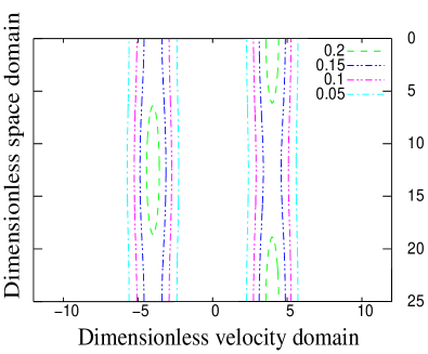
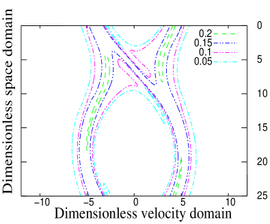
$(a)$	$(b)$

Figure 1. Beams phase space $(a)$ at initial time, $(b)$ at $20$ plasma periods (after saturation)

In Figure 1, two countersteaming beams that are initially well separated in the phase space $(a)$ start to mix together. They finally create a complicated vortex structure, involving wave-particle interactions. This behaviour remains quantitatively the same whatever the transport scheme is (second or fourth order). However with a reduced number of grid points (smaller than $128$ points in velocity), the second order (with limiter (11)) and fourth order schemes present a different behaviour for the total electric energy and total energy.

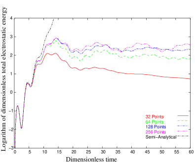
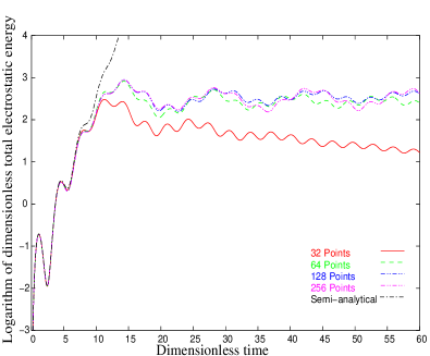
$(a)$	$(b)$

Figure 2. Evolution of the electrostatic energy for $32^{2}$, $64^{2}$, $128^{2}$, $256^{2}$ grid points, and the semi-analytical solution in the linear regime. Results are shown for $(a)$ the second order with limiter (11) and $(b)$ fourth order transport scheme

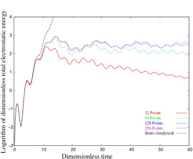
Figure 3. Evolution of the electrostatic energy for $32^{2}$, $64^{2}$, $128^{2}$, $256^{2}$ grid points, and the semi-analytical solution in the linear regime. Results are shown here for the second order scheme with the limiters (12), with $b=2$.

$(a)$	$(b)$

Figure 4. Comparison of the energy evolution for the second (with limiter (11)) and fourth order transport schemes. Results are shown $(a)$ for $32^{2}$ $(b)$ $64^{2}$ grid points

$(a)$	$(b)$

Figure 5. Comparison of the energy evolution for the second (with limiter (12), $b=2$) and fourth order transport schemes. Results are shown $(a)$ for $32^{2}$ $(b)$ $64^{2}$ grid points

For reduced grid resolutions, of $32^{2}$ or $64^{2}$ points, the fourth order scheme proves to be better than the second order one. For $32^{2}$ points, plasma oscillations at the plasma frequency in the nonlinear phase are not reproduced with the second order scheme whereas they can be seen with the fourth order scheme (see Figure 2). Moreover for this resolution, the transition from the linear phase to the nonlinear phase occurs earlier than it should for the second order scheme.
As the grid resolution increases, the accuracy remains better for the fourth order scheme than for the second order one in the nonlinear phase (Figure 2). The convergence toward curves with $128^{2}$ or $256^{2}$ resolution grid is indeed better. We recall that quantities in Figure 2 and 3 are plotted with a logarithmic scale, that smoothes out discrepancies between curves. In addition to these results, the respect of total discrete energy conservation proves to be better for the fourth order scheme than for the second order one at a reduced grid resolution, see Figure 4 and 5.

The use of limiters (12) for the second order scheme introduces accuracy improvements on the convergence behaviour and capture of plasma wave structure at reduce grid resolutions, see Figure 3. However, the energy dissipation remains quantitatively the same as the second order scheme with limiter (11), see Figures 4 and 5.

As this test case requires both a good preservation of invariants and accuracy when nonlinear phenomena occur, we might conclude that the fourth order scheme, with a resolution along each velocity direction greater than $32$ cell, is well suited for our physical applications. The semi-analytical solution in the linear regime shown in Figure 2, using a Green function, brings some improvements compared to the classical validation in the linear regime, based on instabilities growth rates in the linear regime. In particular it discriminates precisely in time the linear and nonlinear phases.

4.3. Test 2: $1D$ X-mode plasma in a magnetic field

This test case stands as a validation in the linear regime for the coupling between Vlasov and Maxwell equations without collisions. A particular initial data is chosen (see the derivation in the appendix B) to trigger an X-mode plasma wave at a well-defined frequency $\omega$. This type of wave presents a mixed polarization (longitudinal and transverse with respect to the magnetic field), that propagates in the plane $P_{\perp}$, perpendicular to the magnetic field direction.

The chosen frequency $\omega$ is a solution of the dispersion relation (127) of the linearized Vlasov-Maxwell equations, introducing the equilibrium state $f^{(0)}\left(\|{\bf v}\|^{2}\right)$. The initial data are chosen such that $f^{(0)}$, $\hat{E}_{1}$, $\hat{E}_{2}$, and $\hat{B}_{3}$ only depend on $\omega$, $B^{(0)}$, $k_{1}\,=\,2\pi/L_{1}$ and $A$; where $\hat{f}_{n}$, $\hat{B}_{3}$, $\hat{E}_{1}$ and $\hat{E}_{2}$ are the reconstructed (in the appendix B) Fourier transforms of the distribution function and electromagnetic fields. The magnetic field $B^{(0)}$ is the nonperturbed magnitude of the magnetic field, $L_{1}$ is the length of the space domain, $A$ is the perturbation amplitude. The initial data can then be constructed with the help of truncated Fourier series

$$\left\{\begin{array}[]{l}\displaystyle{f^{(0)}({x_{1}},{\bf v})\,=\,f^{(0)}(\|{\bf v}\|^{2})\,+\,\sum_{n=-2}^{2}\hat{f}_{n}({\bf v}_{\perp})e^{ik_{1}\,x_{1}\,+\,i\,n\psi}},\quad x_{1}\in(0,L_{1}),\,{\bf v}\in\mathbb{R}^{3},\\ \\ \displaystyle{E_{1}(t,x_{1})\,=\,\hat{E}_{1}\,e^{-i\omega t+ik_{1}x_{1}}},\quad x_{1}\in(0,L_{1})\ ,\\ \\ \displaystyle{E_{2}(t,x_{1})\,=\,\hat{E}_{2}e^{-i\omega t+ik_{1}x_{1}}},\quad x_{1}\in(0,L_{1})\ ,\\ \\ \displaystyle{B(t,x_{1})\,=\;B^{(0)}\,+\,\hat{B}_{3}e^{-i\omega t+ik_{1}x_{1}}},\quad x_{1}\in(0,L_{1}).\end{array}\right.$$

We define $\psi$ as the angle in the cylindrical coordinates for the velocity, defined with respect to the direction of the magnetic field (See appendix B).

The normalisations are defined by relations (32)-(34). We choose $B^{(0)}=2$ and a rather strong amplitude perturbation $A=0.1$ with periodic boundary conditions on the space domain. Also we have set $\beta=v_{th}/c=0.05$. The dispersion relation have been solved for these parameters. One of the solution $\omega\simeq 5.1432$ is injected in the initial data set.

We considered $126$ points along the $1D$ space direction, and $64$ points along each velocity direction ${\bf v}=\,^{t}(v_{1},v_{2},v_{3})$. The dimension of the space domain is $L_{1}\,=\,25$ whereas the truncation of the velocity space occurs at $v_{max}=7$ for each velocity direction. Furthermore, the time step is $\Delta t=1/200$.

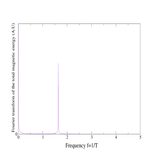
Figure 6. Discrete Fourier spectrum in frequency of the discrete analogous of the total dimensionless magnetic energy $\displaystyle\int_{0}^{L_{1}}\frac{\|B_{3}\|^{2}}{2}dx_{1}$.

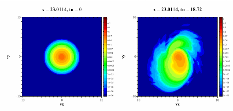
Figure 7. Projection on the $v_{1}-v_{2}$ velocity domain for the distribution function is shown at initial time $t_{n}=0$ and at $t_{n}=18.72$, for a particular point of the space domain, $x_{1}=23.0114$, $v_{3}=0$.

The Fourier spectrum in Figure 6 exhibits a well defined frequency $f=1/T\simeq 1.6375$ (corresponding to a period $T$) for the total magnetic energy, that corresponds to a frequency $f/2$ for the magnetic field oscillations. We finally find $\omega=2\pi\left(\frac{f}{2}\right)\simeq 5.1443$ from the numerical solution, to be compared with the analytical results $5.1432$. This proves a good accuracy of the numerical results, while the distribution function is greatly affected by the magnetic field. As an illustration, we show in Figure 7 how the magnetic field makes the distribution function rotate in the velocity space perpendicular to the magnetic field axis.

5. Approximation of the collision operators

In the following, the presentation is restricted to the space homogeneous equation, for the sake of simplicity,

$$\left\{\begin{array}[]{l}\displaystyle{\frac{\partial f}{\partial t}\,=\,C_{e,e}(f,f)\,+\,C_{e,i}(f)},\\ \\ f(0,{\bf v})\,=\,f^{(0)}({\bf v}),\end{array}\right.$$

where $C_{e,e}(f,f)$ and $C_{e,i}(f)$ are given by (36).

5.1. Discretization of the Lorentz operator

We consider $f_{\bf j}$ an approximation of the distribution function $f{\bf(v_{j})}$ and introduce the operator ${\bf D}$, which denotes a discrete form of the usual gradient operator $\nabla_{\bf v}$ whereas ${\bf D^{*}}$ represents its formal adjoint, which represents an approximation of $-\nabla_{\bf v}\cdot$. Therefore, for any test sequence $(\psi_{\bf j})_{{\bf j}\in\mathbb{Z}^{3}}$, we set $({\bf D}\psi_{\bf j})_{{\bf j}\in\mathbb{Z}^{3}}$ as a sequence of vectors of $\mathbb{R}^{3}$

$${\bf D}\psi_{\bf j}\,=\,{}^{t}(D_{1}\psi_{\bf j},D_{2}\psi_{\bf j},D_{3}\psi_{\bf j})\in\mathbb{R}^{3},$$

where $D_{s}$ is an approximation of the partial derivative $\frac{\partial}{\partial v_{s}}$ with $s\in\{1,2,3\}$. In order to preserve the property of decreasing entropy at the discrete level, we use the log weak formulation of the Lorentz operator [14]

$$\int_{\mathbb{R}^{3}}\,C_{e,i}(f)({\bf v})\,\psi({\bf v})\,{\bf dv}\,=\,-\int_{\mathbb{R}^{3}}\Phi({\bf v})\,f({\bf v})\,\nabla_{\bf v}\log(f({\bf v}))\cdot\nabla_{\bf v}\psi({\bf v})\,{\bf dv},$$

where $\Phi$ is given by (6) and $\psi$ is a smooth test function. Then, using the notations previously introduced, the discrete operator $C_{e,i}^{\Delta v}(f)$ is given by

(37) $$C_{e,i}^{\Delta v}(f)({\bf v_{j}})\,=\,-{\bf D^{*}}\left[\frac{1}{\|{\bf v}_{\bf j}\|^{3}}\,S({\bf\tilde{v}_{j}})\,f_{\bf j}\,{\bf D}(\log(f_{\bf j}))\,\right],$$

where $S(\tilde{{\bf v_{j}}})$ is the following matrix

$$S(\tilde{{\bf v_{j}}})\,=\,\|\tilde{{\bf v_{j}}}\|^{2}\,{\rm Id}\,-\,\tilde{{\bf v_{j}}}\otimes\tilde{{\bf v_{j}}}.$$

Now, ${\bf\tilde{v}_{j}}$ has to satisfy the discrete conservation of energy

(38) $$\frac{D_{1}(\|{\bf{v}_{j}}\|^{2})}{{\bf\tilde{v}}_{j_{1}}}\,=\,\frac{D_{2}(\|{\bf{v}_{j}}\|^{2})}{{\bf\tilde{v}}_{j_{2}}}\,=\,\frac{D_{3}(\|{\bf{v}_{j}}\|^{2})}{{\bf\tilde{v}}_{j_{3}}}.$$

Then, we consider the $8$ uncentered operators ${\bf D^{{\bf\epsilon}}}$, with the formalism:

$${\bf D^{{\bf\epsilon}}}\,=\,{}^{t}(D^{{\epsilon_{1}}}_{1},D^{{\epsilon_{2}}}_{2},D^{{\epsilon_{3}}}_{3}),$$

with ${\bf\epsilon}={}^{t}(\epsilon_{1},\epsilon_{2},\epsilon_{3})$, and $\epsilon_{i}\in\{+1,-1\}$ for $i\in\{1,2,3\}$. More precisely, the operator $D^{\epsilon_{i}}$ is the forward uncentered discrete operator if $\epsilon_{i}=+1$ and the backward uncentered discrete operator if $\epsilon_{i}=-1$:

(42) $${\bf D^{\epsilon}}{\bf\Psi}_{{\bf j}}=\frac{1}{\Delta v}\left(\begin{array}[]{ccc}\epsilon_{1}[\Psi_{j_{1}+\epsilon_{1}}-\Psi_{j_{1}}]\\ \epsilon_{2}[\Psi_{j_{2}+\epsilon_{2}}-\Psi_{j_{2}}]\\ \epsilon_{3}[\Psi_{j_{3}+\epsilon_{3}}-\Psi_{j_{3}}]\end{array}\right)$$

This $8$ operators respectively match to $8$ expressions of ${\bf\tilde{v}_{j}^{\epsilon}}$, following (38)

$${\bf\tilde{v}_{j}^{\epsilon}}\,=\,\frac{1}{2}\left({\bf{v}_{j}}\,+\,{\bf{v}_{j+{\bf\epsilon}}}\right).$$

This choice has been made to avoid the use of the centered discrete operator that conserves non physical quantities. On the other hand, the uncentered operators, taken separately, introduce some artificial unsymmetry in the distribution function leading to a loss of accuracy when coupling to Maxwell equations. To overcome these difficulties, following the idea of [9], we introduce a symmetrization of the discrete operator based on the averaging over the eight uncentered discretizations:

$$\displaystyle C^{\Delta v}_{e,i}(f)({\bf v_{j}})\,=\,\frac{1}{8}\sum_{{\bf\epsilon}}C_{e,i}^{\epsilon}(f)$$

$$\displaystyle C_{e,i}^{\epsilon}(f)=-{\bf D^{*,{\bf\epsilon}}}\left[\frac{1}{\|{\bf v_{j}}\|^{3}}S({\bf\tilde{v}_{j}^{{\bf\epsilon}}})\,f_{\bf j}\,{\bf D^{{\bf\epsilon}}}(\log(f_{\bf j}))\right].$$

This final expression will introduce an additional discrete symmetry property compared to the operator presented in [12].

We now present the discrete properties for the electron-ion collision operator. We have the classical properties: mass and energy preservation, an entropy decreasing behaviour, the positivity preservation of the distribution function in a finite time sequence. The proofs are not detailed here but can be deduced easily from those presented in [12]. The difference stands in the fact that we obtain the operator as an average over the full set of the uncentered operators (instead of an average over two operators). This modification allows to get a discrete analogous of the symmetry property presented in Proposition 2.1:

Proposition 5.1.

Under the condition (38) on ${\bf\tilde{v}_{j}}$, the discretization (5.1) to the Lorentz operator (5) satisfies the following properties,

• it preserves mass and energy,

• it decreases discrete entropy

  $$H(t)\,=\,\Delta v^{3}\,\sum_{{\bf j}\in\mathbb{Z}^{3}}f_{{\bf j}}(t)\,\log(f_{{\bf j}}(t)),$$

• there exists a time-sequence $\Delta t_{n}$ such that the scheme

  $$f_{{\bf j}}^{n+1}\,=\,f_{{\bf j}}^{n}\,+\,\Delta t\,C^{\Delta v}_{e,i}(f)({\bf v_{j}}),$$

  defines a positive solution at any time i.e. $\sum_{n}t_{n}\,=\,+\infty$.

Furthermore, if $f_{\bf j}$ is symmetric with respect to $0$ in the direction $j_{k}$ at time $t^{n}$, then this property is preserved at time $t^{n+1}$,

(43) $$\sum_{{\bf j}\in\mathbb{Z}^{3}}C^{\Delta v}_{e,i}(f)({\bf v_{j}})v_{j_{k}}\Delta v^{3}\,=\,0.$$

Proof:  We prove the last property and rewrite the operator (5.1) in a different manner, assuming we have a symmetry along the velocity direction $v_{j_{k}}$

(44) $$C^{\Delta v}_{e,i}(f)({\bf v_{j}})\,=\,\frac{1}{8}\sum_{\epsilon}C_{e,i}^{{\bf\epsilon}}(f)({\bf v_{j}})\,=\,\frac{1}{4}\left[\sum\frac{1}{2}\left(C_{e,i}^{{\bf\epsilon}^{+,(k)}}({\bf v_{j}})+C_{e,i}^{{\bf{\epsilon}}^{-,(k)}}({\bf v_{j}})\right)\right],$$

where the notation ${\bf\epsilon}^{\pm,(k)}$ refers to

(47) $$\,\left\{\begin{array}[]{ll}{\bf\epsilon}^{\pm,(k)}_{i}=\pm 1&\textrm{ if }i=k,\\ {\bf\epsilon}^{\pm,(k)}_{i}={\bf\epsilon}_{i}&\textrm{ if }i\neq k.\end{array}\right.$$

We are interested in the cancellation of the operator $\displaystyle\sum_{{\bf j}\in\mathbb{Z}^{3}}C^{\Delta v}_{e,i}(f)({\bf v_{j}})v_{j_{k}}$. This is equivalent to the cancellation of

$$Q^{{(k)}} := \sum_{{\bf j}\in\mathbb{Z}^{3}}\left(C_{e,i}^{{\bf\epsilon}^{+,(k)}}({\bf v_{j}})+C_{e,i}^{{\bf{\epsilon}}^{-,(k)}}({\bf v_{j}})\right)v_{j_{k}}$$

$$= \sum_{{\bf j}\in\mathbb{Z}^{3}}\frac{1}{\|{\bf v_{j}}\|^{3}}f_{\bf j}\left[S(\tilde{\bf v_{j}}^{{\bf\epsilon}^{+,(k)}}){\bf D}^{{\bf\epsilon}^{+,(k)}}\log(f_{\bf j})\right]\cdot{\bf D}^{{\bf\epsilon}^{+,(k)}}v_{j_{k}}$$

$$+ \sum_{{\bf j}\in\mathbb{Z}^{3}}\frac{1}{\|{\bf v_{j}}\|^{3}}f_{\bf j}\left[S(\tilde{\bf v_{j}}^{{\bf\epsilon}^{-,(k)}}){\bf D}^{{\bf\epsilon}^{-,(k)}}\log(f_{\bf j})\right]\cdot{\bf D}^{{\bf\epsilon}^{-,(k)}}v_{j_{k}}.$$

Then, since ${\bf D}^{{\bf\epsilon}^{+,(k)}}v_{j_{k}}={\bf D}^{{\bf\epsilon}^{-,(k)}}v_{j_{k}}={\bf e_{k}}$, it yields

$$Q^{{(k)}} = \sum_{{\bf j}\in\mathbb{Z}^{3}}\frac{1}{\|{\bf v_{j}}\|^{3}}f_{\bf j}\left(\sum_{i\neq k}\left(\tilde{v}_{j_{i}}^{{\epsilon}^{+,(k)}_{i}}\right)^{2}\right)D^{\epsilon_{k}^{+,(k)}}(\log(f_{\bf j}))$$

$$- \sum_{{\bf j}\in\mathbb{Z}^{3}}\frac{1}{\|{\bf v_{j}}\|^{3}}f_{\bf j}\tilde{v}_{j_{k}}^{\epsilon_{k}^{+,(k)}}\left(\sum_{i\neq k}\tilde{v}_{j_{i}}^{\epsilon_{i}^{+,(k)}}D^{\epsilon_{i}^{+,(k)}}(\log f_{\bf j})\right)$$

$$- \sum_{{\bf j}\in\mathbb{Z}^{3}}\frac{1}{\|{\bf v_{j}}\|^{3}}f_{\bf j}\left(\sum_{i\neq k}\left(\tilde{v}_{j_{i}}^{{\epsilon}^{-,(k)}_{i}}\right)^{2}\right)D^{{\epsilon}^{-,(k)}_{k}}(\log(f_{\bf j}))$$

$$- \sum_{{\bf j}\in\mathbb{Z}^{3}}\frac{1}{\|{\bf v_{j}}\|^{3}}f_{\bf j}\tilde{v}_{j_{k}}^{{\epsilon}^{-,(k)}_{k}}\left(\sum_{i\neq k}\tilde{v}_{j_{i}}^{{\epsilon}^{-,(k)}_{i}}D^{{\epsilon}^{-,(k)}_{i}}(\log f_{\bf j})\right).$$

Then using definition (47) and the symmetry of $f_{\bf j}^{n}$ with respect to $0$ in the velocity direction $v_{j_{k}}$, we obtain $Q^{{(k)}}=0$. Then multiplying (44) by $v_{j_{k}}$ and integrating in the full velocity space gives the relation (43). This relation implies that $f_{\bf j}^{n+1}$ is symmetric with respect to 0 in the direction $v_{j_{k}}$. $\Box$

5.2. Discrete Landau operator

We consider the discretization of the FPL operator (4) on the whole 3D velocity space. It is based on the entropy conservative discretization introduced in [14], where a discrete weak log form of the FPL operator is used. This discretization yields:

(48) $$\left\{\begin{array}[]{l}\displaystyle{\frac{df_{\bf j}(t)}{dt}=\left({\bf D^{*}}\rho(t)\right)_{\bf j}\qquad{\bf j}\in\mathbb{Z}^{3},}\\ \\ \displaystyle{\rho(t)=\Delta v^{3}\sum_{{\bf m}\in\mathbb{Z}^{3}}f_{\bf j}(t)f_{\bf m}(t)\Phi({\bf v_{j}}-{\bf v_{m}})\left({\bf D}(\log(f(t))_{\bf j}-{\bf D}(\log f(t))_{\bf m}\right),}\end{array}\right.$$

where ${\bf D}$ stands for a downwind or upwind finite discrete operator approximating the usual gradient operator $\nabla_{\bf v}$. This uncentered approximation ensures that the only equilibrium states are the discrete Maxwellian. The use of centered discrete operators would have lead to non physical conserved quantities. The discretization of the FPL operator is then obtained as the average over uncentered operators, but here for a different reason as in the previous section, on the electron-ion collision operator discretization. In [10], the scheme is rewritten as the sum of two terms: a second order approximation and an artificial viscosity term in $\Delta v^{2}$ which kills spurious oscillations. However the computational cost of a direct approximation of (48) remained too high. Therefore, a multigrid technique has been used. We refer to [10] and [11] for the details of the implementation on the FPL operator. Nevertheless, these latter approaches introduce a new approximation than can affect accuracy. Based on [27], Crouseilles and Filbet proposed another approach and noticed that the discrete FPL operator (48) in the Fourier space can be written as a discrete convolution, which directly gives a fast algorithm. Here we adopt the multigrid method, detailed in [10], that has a complexity of order ${O}(n_{v}^{3}\log n_{v}^{3})$.

This discrete approximation preserves positivity, mass, momentum, energy, and decreases the entropy. Moreover the discrete equilibrium states are the discrete Maxwellian.

6. Numerical results

6.1. Scaling with collision frequency

For the analysis of collisional processes, a new scaling is introduced here, that allows time steps to be of the order of the electron-ion collision time. In order to account for transport phenomena occuring at the collision time scale, several parameters are required: the electron-ion collision frequency $\nu_{e,i}$, the associated mean free path $\lambda_{e,i}$, the thermal velocity $v_{th}$, and the cylotron frequency $\omega_{ce}$

(49) $$\nu_{e,i}=\frac{Z\,n_{0}\,e^{4}\,\ln\Lambda}{8\,\pi\,\epsilon_{0}^{2}\,m_{e}^{2}\,v_{th}^{3}}\,,\quad\lambda_{e,i}=\frac{v_{th}}{\nu_{e,i}}\,,\quad v_{th}=\sqrt{\frac{\kappa_{B}T_{0}}{m_{e}}}\,,\quad\omega_{ce}={\frac{eB}{m_{e}}}\,,$$

These parameters enable us to define the dimensionless parameters with tilde.

• Dimensionless time, space and velocity, respectively

  (50) $$\tilde{t}=\nu_{e,i}t,\quad\tilde{x}={x}/{\lambda_{e,i}},\quad\tilde{v}={v}/{v_{th}}.$$

• Dimensionless electric field, magnetic field, and distribution function, respectively

  (51) $$\tilde{E}=\frac{eE}{m_{e}v_{th}\nu_{e,i}}\,,\quad\tilde{B}=\frac{eB}{m_{e}\nu_{e,i}}=\frac{\omega_{ce}}{\nu_{e,i}}\,,\quad\tilde{f_{e}}=f_{e}\frac{v_{th}^{3}}{n_{0}}.$$

This leads to the following dimensionless equations

(52) $$\left\{\begin{array}[]{l}\displaystyle{\frac{\partial f_{e}}{\partial t}+\nabla_{{\bf x}}\cdot\left({\bf v}f_{e}\right)-\nabla_{\bf v}\cdot\left(({\bf E}+{\bf v}\times{\bf B})f_{e}\right)=\frac{1}{Z}C_{e,e}(f_{e},f_{e})+C_{e,i}(f_{e}),}\\ \\ \displaystyle{\frac{\partial{\bf E}}{\partial t}-\frac{1}{{\beta}^{2}}\nabla_{\bf x}\times{\bf B}=\frac{1}{{\alpha}^{2}}n{\bf u},}\\ \\ \displaystyle{\frac{\partial{\bf B}}{\partial t}+\nabla_{\bf x}\times{\bf E}=0,}\\ \\ \displaystyle{\nabla_{\bf x}\cdot{\bf E}=\frac{1}{{\alpha}^{2}}(1-n),}\\ \\ \displaystyle{\nabla_{\bf x}\cdot{\bf B}=0,}\end{array}\right.$$

where $\alpha=\nu_{e,i}/\omega_{pe}$ and $\beta=v_{th}/c$. The collision terms $C_{e,e}(f_{e},f_{e})$ and $C_{e,i}(f_{e})$ are given in (36).

6.2. 1D temperature gradient test case

In the context of laser produced plasma, the heat conduction is the leading mecanism of energy transport between the laser energy absoption zone and the target ablation zone.
In such a system, the parameters of importance for the heat flux are

• The effective electron collision mean free path $\lambda_{e}$.

• The electron temperature gradient length $\lambda_{T}$.

• The magnetic field $B$ and its orientation with respect to $\nabla T$.

These parameters enable to distinguish different regimes of transport, according to the Knudsen and the Hall parameters.
The Knudsen number $K_{n}$ is a mesure of the thermodynamical non-equilibrium of the system

(53) $$K_{n}=\frac{\lambda_{e}}{\lambda_{T}}.$$

A regime characterized by $K_{n}\rightarrow 0$ refers to an hydrodynamical descripion, whereas a regime characterized by $K_{n}\geq 1$ refers to a kinetic description, where the nonlocal phenomena appear. The parameters for ICF imply $K_{n}\geq 0.1$, while the classical, local approach fails at $K_{n}\geq 0.01$. This premature failure of the classical diffusion approach in plasma is explained by a specific dependence of the electron mean free path on their energy. In our applications the energy is transported by the fastest electrons, which have a much longer mean free path.
The Hall parameter $\chi=\omega_{c}\tau$ quantifies the relative importance of magnetic and collisional effects. $\omega_{c}=eB/m_{e}$ is the electron cyclotron frequency and $\tau$ the mean electron-ion collision time

(54) $$\tau=\frac{3}{4}\frac{16\pi^{2}\epsilon_{0}^{2}\sqrt{m_{e}}T_{e}^{3/2}}{\sqrt{2\pi}n_{i}Z^{2}e^{4}ln\Lambda}.$$

For this test case, a simple gradient temperature configuration is shown in figure (8), modelling the following situation: through a layer of homogeneous plasma, a laser deposits its energy on the hot temperature side and the absorbed energy is transported with electrons to the cold temperature side.

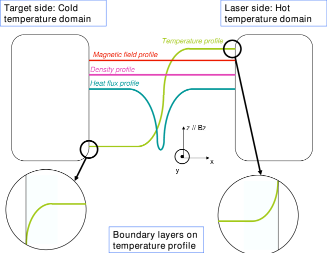
Figure 8. Initial configuration for the temperature gradient test case: a temperature profile is considered between to two domains of plasma with particles at thermodynamical equilibrium. Zero current boundary conditions enable to maintain mass conservation. A heat flux is generated wherever there is a nonzero temperature gradient, as well as boundary layers on the heat flux, temperature, and electromagnetic profiles.

Let us define the average over velocity of a function $A({\bf v})$

(55) $$<A>=\frac{1}{n_{e}}\int_{\mathbb{R}^{3}}Af{\bf dv}\quad,$$

where $n_{e}(t,{\bf x})=\displaystyle\int_{\mathbb{R}^{3}}f(t,{\bf x},{\bf v}){\bf dv}$ is the density of electrons.

Following [6, 16], we introduce the macroscopic quantities

(61) $$\left\{\begin{array}[]{l}\displaystyle{\bf j}=q_{e}n_{e}\left<{\bf v}\right>,\\ \\ \displaystyle{\bf q}=\frac{1}{2}m_{e}n_{e}\left<({\bf v\cdot v}){\bf v}\right>,\\ \\ \displaystyle{\bf R}=\int_{\mathbb{R}^{3}}m_{e}{\bf v}C_{e,i}(f_{e}){\bf dv},\end{array}\right.$$

(67) $$\left\{\begin{array}[]{l}\displaystyle p=n_{e}T_{e}=\frac{1}{3}m_{e}n_{e}\left<({\bf v-<{\bf v}>})\cdot({\bf v-<{\bf v}>})\right>,\\ \\ \displaystyle{\bf\Pi}=\frac{1}{3}m_{e}n_{e}\left<({\bf v-<{\bf v}>})\otimes({\bf v-<{\bf v}>})\right>-p{\bf I},\\ \\ \displaystyle{\bf q_{loc}}=\frac{1}{2}m_{e}n_{e}\left<\left[({\bf v-<{\bf v}>})\cdot({\bf v-<{\bf v}>})\right]({\bf v-<v>})\right>.\end{array}\right.$$

There, ${\bf j}$ is the electric current, ${\bf q}$ the total heat flow, ${\bf R}$ the friction force accounting for the transfer of momentum from ions to electrons in collisions, $T_{e}$ is the temperature, $p$ is the scalar intrinsic pressure, ${\bf\Pi}$ is the stress tensor, ${\bf q_{loc}}$ is the intrinsic heat flow and ${\bf I}$ the unit diagonal tensor.
Quantities $p$, ${\bf\Pi}$ and ${\bf q_{loc}}$ are defined in the local reference frame of the electrons, whereas ${\bf j}$, ${\bf q}$ and ${\bf R}$ are defined relative to the ion center of mass frame. Ions are supposed to be at rest. We have the relation

(68) $${\bf q_{loc}}={\bf q}+{\bf j}\cdot(\frac{5}{2}p{\bf I}+{\bf\Pi})/(n_{e}e)+{\bf j}(\frac{1}{2}m_{e}n_{e}<{\bf v}>^{2})/(n_{e}e).$$

The validation of our Fokker-Planck solver in the domain close to the hydrodynamical regime (local regime) requires knowledge of transport coefficients. Following the formalism of Braginskii [6] for the transport relations, the transport coefficients in the hydrodynamical regime have been calculated by Epperlein in [16]. These coefficients ${\bf\alpha_{ep}}$, ${\bf\beta_{ep}}$, ${\bf\kappa_{ep}}$, are the electrical resistivity, thermoelectric and thermal conductivity tensors, respectively. From these quantities, we are able to compare the heat flux and electric field issued from the Fokker-Planck solver to those calculated analytically in [16], in the local regime.
The classical derivation procedure to obtain the transport coefficients involves the linearization of the Fokker-Planck-Landau equation, assuming the plasma to be close to the thermal equilibrium. The distribution function is approximated using a truncated Cartesian tensor expansion $\displaystyle f(t,{\bf x},{\bf v})=f^{(0)}(\|{\bf v}\|^{2})+\frac{\bf v}{\|{\bf v}\|^{2}}\cdot{\bf f^{(1)}}(t,{\bf x},{\bf v})$. Following [16], ${\bf\Pi}$ and $m_{e}n_{e}<{\bf v}>^{2}$ are neglected. Then considering appropriate velocity moments of ${\bf f^{(1)}}$, electric fields and heat fluxes are expressed as a function of thermodynamical variables. The coefficients of proportionality, in the obtained relations, are defined as the transport coefficients.
Several notations can be used, depending on the chosen thermodynamical variables. Adopting the Braginskii notations, we obtain

(72) $$\left\{\begin{array}[]{l}\displaystyle{\bf R}={\bf\nabla}p+en_{e}{\bf E}-{\bf j}\times{\bf B}=\frac{{\bf\alpha_{ep}}\cdot{\bf j}}{n_{e}e}-{\bf\beta_{ep}\cdot\nabla}T_{e},\\ \\ \displaystyle{\bf q}=-\frac{5}{2}\frac{\bf j}{e}T_{e}-{\bf\kappa_{ep}}\cdot{\bf\nabla}T_{e}-{\bf\beta_{ep}}\cdot{\bf j}\frac{\bf T_{e}}{e}.\end{array}\right.$$

We want to compare of the results of the solver with the analytical electric fields and heat fluxes in the local regime. For that purpose, we use the values of coefficients, for $Z=1$, that are tabulated in [16]. As for the components of these tensors, we make use of the standard notations $||$, $\perp$, and $\wedge$. Directions denoted with $||$ and $\perp$ are respectively parallel and perpendicular to the magnetic field. Consequently, the parallel and perpendicular components of a vector ${\bf u}$ are respectively $u_{||}={\bf b}({\bf u}\cdot{\bf b})$ and $u_{\perp}={\bf b}\times({\bf b}\times{\bf u})$, where ${\bf b}$ is the unit vector in the direction of the magnetic field. The direction defined by the third direction in a direct orthogonal frame is denoted by $\wedge$. In the system (72), the relation between any transport coefficient tensor ${\bf\varphi}$ and vector ${\bf u}$ is defined by

(73) $${\bf\varphi}\cdot{\bf u}=\varphi_{||}{\bf b}({\bf b\cdot u})+\varphi_{\perp}{\bf b}\times({\bf u}\times{\bf b})\pm\varphi_{\wedge}{\bf b}\times{\bf u}\ ,$$

where the negative sign applies only in the case ${\bf\varphi}={\bf\alpha_{ep}}$. These coefficients can be expressed in dimensionless form

(79) $$\left\{\begin{array}[]{l}\displaystyle{\bf\alpha^{c}_{ep}}={\bf\alpha_{ep}}\frac{\tau}{m_{e}n_{e}},\\ \\ \displaystyle{\bf\beta^{c}_{ep}}={\bf\beta_{ep}},\\ \\ \displaystyle{\bf\kappa^{c}_{ep}}={\bf\kappa_{ep}}\frac{m_{e}}{n_{e}\tau T_{e}}.\end{array}\right.$$

The dimensionless transport coefficients ${\bf\alpha_{ep}^{c}}$, ${\bf\beta_{ep}^{c}}$, ${\bf\kappa_{ep}^{c}}$ are functions of $Z$ and the Hall parameter $\chi=\omega_{c}\tau$ only.
The heat flux and the electric field in (72) can then be rewritten in terms of dimensionless quantities, for the particular 1D geometry of our temperature gradient configuration. In that case, the normalizations using a collision frequency (49)-(51) are used.

(87) $$\left\{\begin{array}[]{l}\displaystyle q_{1}=-\frac{5}{2}T_{e}n_{e}^{-1}j_{1}-\chi T_{e}B_{3}^{-1}\nabla_{x_{1}}T_{e}{\bf\kappa_{ep,\perp}^{c}}-T_{e}\left({\bf\beta_{ep,\perp}^{c}}j_{1}-{\bf\beta_{ep,\wedge}^{c}}j_{2}\right),\\ \\ \displaystyle q_{2}=-\frac{5}{2}T_{e}n_{e}^{-1}j_{2}-\chi T_{e}B_{3}^{-1}\nabla_{x_{1}}T_{e}{\bf\kappa_{ep,\wedge}^{c}}-T_{e}\left({\bf\beta_{ep,\perp}^{c}}j_{2}+{\bf\beta_{ep,\wedge}^{c}}j_{1}\right),\\ \\ \displaystyle E_{1}={n_{e}}^{-1}j_{2}B_{3}-n_{e}^{-1}\nabla_{x_{1}}p-\nabla_{x_{1}}T_{e}{\bf\beta_{ep,\perp}^{c}}+{n_{e}}^{-1}B_{3}{\chi}^{-1}({\bf\alpha_{ep,\perp}^{c}}j_{1}+{\bf\alpha_{ep,\wedge}^{c}}j_{2}),\\ \\ \displaystyle E_{2}=-{n_{e}}^{-1}j_{1}B_{3}-\nabla_{x_{1}}T_{e}{\bf\beta_{ep,\wedge}^{c}}+{n_{e}}^{-1}B_{3}{\chi}^{-1}({\bf\alpha_{ep,\perp}^{c}}j_{2}-{\bf\alpha_{ep,\wedge}^{c}}j_{1}).\end{array}\right.$$

The Hall parameter $\chi$ is expressed in terms of the dimensionless quantities $B_{3}$ and $T_{e}$:

(88) $$\chi=\frac{3\sqrt{\pi}}{2\sqrt{2}}\frac{B_{3}T_{e}^{3/2}}{Z}.$$

6.2.1. Electron transport in the local regime

In order to validate the numerical scheme in the local regime, we compare the heat flux ${\bf Q_{FP}}$ and electric field ${\bf E_{FP}}$ computed from the numerical solution, with those analytically (denoted by ${\bf Q_{BR}}$ and ${\bf E_{BR}}$) computed from the system (87). The transport coefficients ${\bf\alpha_{ep}}$, ${\bf\beta_{ep}}$, ${\bf\kappa_{ep}}$ have been tabulated in [16].

In this test case the source term can be considered stiff; the discretization of the collision operator is then of crucial importance and its accuracy can be tested. Moreover we provide, in this local regime, with validation results for a wide range of Hall parameters corresponding to ICF applications.
The initial temperature gradient $T_{e}(x_{1})$ has the form of a step

(92) $$T_{e}(x_{1})=\left\{\begin{array}[]{l}\displaystyle T_{e}^{R}(x_{1})\qquad\mbox{if}\quad x_{1}>x_{1}^{m}\ ,\\ \\ \displaystyle T_{e}^{L}(x_{1})\qquad\mbox{else}\ ,\end{array}\right.$$

where $T_{e}^{R}$ and $T_{e}^{L}$ are third order polynomials in $x_{1}-x_{1}^{m}$, $x_{1}$ standing for the space coordinate and $x_{1}^{m}$ for the mid-point of the 1D domain. The coefficients of these polynomials are chosen such as they verify the following conditions at $x_{1}^{m}$

(96) $$\left\{\begin{array}[]{l}\displaystyle\frac{\partial T_{e}^{L}}{\partial x_{1}}(x_{1}^{m})=\frac{\partial T_{e}^{R}}{\partial x_{1}}(x_{1}^{m})=\frac{T_{R}-T_{L}}{(x_{1}^{R}-x_{1}^{L})/\lambda},\\ \\ \displaystyle T_{e}^{L}(x_{1}^{m})=T_{e}^{R}(x_{1}^{m})=\frac{T_{R}+T_{L}}{2},\end{array}\right.$$

and at the boundaries

(102) $$\left\{\begin{array}[]{l}\displaystyle T_{e}^{L}(x_{1}^{L})=T_{L},\\ \\ \displaystyle T_{e}^{R}(x_{1}^{R})=T_{R},\\ \\ \displaystyle\frac{\partial T_{e}^{L}}{\partial x_{1}}(x_{1}^{L})=\frac{\partial T_{e}^{R}}{\partial x_{1}}(x_{1}^{R})=0,\end{array}\right.$$

where $T_{L}$ (resp. $T_{R}$) is the initial temperature of the leftmost (resp. rightmost) point $x_{1}^{L}$ (resp. $x_{1}^{R}$) of the domain. $\lambda$ is a parameter that determines the initial stiffness of the temperature gradient.

The simulations were performed with the following parameters: the uniform magnetic field $B_{3}(t=0,x_{1})=0.001,0.01,0.1,1$, the size of the dimensionless domain $L=x_{1}^{R}-x_{1}^{L}=5400$, $2\times v_{max}=12$, the ion charge $Z=1$, the frequency ratio $\nu_{e,i}/\omega_{pe}=0.01$, the electron thermal velocity such as $v_{th}/c=0.05$. The initial electric field is zero over the domain: $E_{1}(t=0,x_{1})=E_{2}(t=0,x_{1})=0$. The initial distribution function is a Maxwellian depending on the local temperature, the density being constant over the domain. The initial temperature profile is chosen such as $T_{L}=0.8$, $T_{R}=1.2$ and $\lambda=10$. This set of parameters enable us to consider the local regime, close to the hydrodynamics (the Knudsen number is about $1/500$). The dimensionless time step and meshes size are $\Delta t=1/500$, $\Delta x_{1}=L/126$, $\Delta v=2v_{max}/32$ respectively. The grid has $126$ points in space and $32^{3}$ points in velocity; $42$ processors were used for each simulation (CEA-CCRT-platine facility). Domain decomposition on the space domain allows each processor to deal only with $3$ points in space. The fourth order scheme on the transport part has been used.

Results are presented in Figures 9-11. The typical run time is 24 hours for 40 collision times, with that set of parameters. The maximum difference between the numerical and the analytical solution are less than $10\%$ for longitudinal macroscopic quantities (heat flux and electric field); $20\%$ for transverse ones. Transverse quantities have only been considered for simulations presented in Figures 10 and 11 where the magnetic field was strong enough so that

• The establishment of transverse heat flux can be acheived during the simulation time.

• Transverse quantities cannot be considered negligible compared to longitudinal ones.

These conditions where fulfilled for $B_{3}=0.1,1$.
In Figures 9-11, only results for simulations with $B_{3}=0.001$, $B_{3}=0.1$, $B_{3}=1$ are shown, respectively. The simulation with $B_{3}=0.01$ proved to show no significance differences with those with $B_{3}=0.001$.

Figure 9. Longitudinal (along the temperature gradient) ratios $\frac{\max_{x_{1}}(Q_{FP})}{\max_{x_{1}}(Q_{BR})}$ (dashed curve) and $\frac{\max_{x_{1}}(E_{FP})}{\max_{x_{1}}(E_{BR})}$ (oscillating curve) are shown against the dimensionless time. The dimensionless magnetic field is $B_{3}=0.001$. Asymptotic behaviour, where the flux is well established, shows good agreement (less than $5\%$ error) with analytical solution (Braginskii formalism), denoted by subscript $\small{BR}$.

(a) Longitudinal	(b) Transverse

Figure 10. Ratios $\frac{\max_{x_{1}}(Q_{FP})}{\max_{x_{1}}(Q_{BR})}$ (curve in bold) and $\frac{\max_{x_{1}}(E_{FP})}{\max_{x_{1}}(E_{BR})}$ (dashed curve) are shown against the dimensionless time. Longitudinal quantities (along the temperature gradient) are shown in (a), with about $10\%$ accuracy in the asymptotics. Transverse quantities are shown in (b), with about $20\%$ accuracy in the asymptotics. The dimensionless magnetic field is $B_{3}=0.1$.

(a) Longitudinal	(b) Transverse

Figure 11. Ratios $\frac{\max_{x_{1}}(Q_{FP})}{\max_{x_{1}}(Q_{BR})}$ (curve in bold) and $\frac{\max_{x_{1}}(E_{FP})}{\max_{x_{1}}(E_{BR})}$ (dashed curve) are shown against the dimensionless time. Longitudinal quantities (along the temperature gradient) are shown in (a), with about $5\%$ accuracy in the asymptotics. Transverse quantities are shown in (b), with about $20\%$ accuracy in the asymptotics. The dimensionless magnetic field is $B_{3}=1$.

Results shown Figures 9-11 are revealing an important transient phase before the establishment of a stationary regime. The oscillations are enforced by the magnetic field, Figure 11. The oscillating electric fields are the consequence of the plasma waves excited by our initial conditions; they are damped in a few electron-ion collision times. These plasma oscillations are smoothed out by the large time steps we used in simulations, allowed by the implicit treatment of the Maxwell equations. However this has a little importance on the asymptotic values and a little importance for accuracy. With a larger magnetic field Figure 11, we observe frequency modulations at $\omega_{c}=\nu_{e,i}$ (corresponding to $B_{3}=1$), both on electric fields and heat fluxes.

In order to investigate Larmor radius effects for simulations presented in Figures 10 and 11, we refined the space grid below the dimensionless Larmor radius $r_{L}=B_{3}^{-1}$. Therefore, simulation presented in Figure 10 has been done again with the same parameters on the same time period: we have refined the grid to $1260$ points in space (420 processors). In the same manner, the simulation presented in Figure 11 has been done again with $6300$ grid points in space (2100 processors) and $\Delta t=1/1000$ (C.F.L. condition), during the same time period. The results prove to be similar to those with coarse space grids, both for macroscopic quantities and distribution functions. We thus show no dependence on the Larmor radius. Here we remark that the cyclotron frequency is always resolved. The time steps are constrained, for most of the cases we treat, by the C.F.L. on collision operators.

6.2.2. Electron transport in the nonlocal regime

The departure of transport coefficients from their local values is of interest here. We restrict ourselves to cases where the magnetic field is zero. Then it is possible to obtain directly the ratio of effective thermal conductivity to the Spitzer-Härm conductivity $\kappa/\kappa_{SH}$ by the relation:

(103) $$\frac{\kappa}{\kappa_{SH}}=\frac{q_{1}}{q_{SH}}.$$

The Spitzer-Härm regime refers to a local regime with no magnetic field. In (103), $q_{1}$ is calculated from the numerical solution and $q_{SH}$ from (87) in the Spitzer-Härm limit.
Transport coefficients are extracted from the domain where the flux and temperature gradient are maximum.
The wavelength of the temperature perturbation $k\lambda_{e,i}$ in the Fourier space is computed from the gradient temperature profile. This enables to obtain a range (due to an uncertainty) for $k\lambda_{e,i}$ corresponding to this temperature gradient.
The results will be compared with the analytical formula from [17]

(104) $$\frac{\kappa}{\kappa_{SH}}=\frac{1}{1+(30k\lambda_{e,i}\beta)^{4/3}},$$

(105) $$\beta=\left(\frac{3\pi}{128}\frac{3.2(0.24+Z)}{(1+0.24Z)}\right)^{1/2}\frac{Z^{1/2}}{2}.$$

The comparison between the numerical results and the analytical solution are in good agreement. The three runs have been performed with the same precision for the temperature gradient.

Parameters	RUN1	RUN2	RUN3
Size of the domain	5400	540	540
Stiffness parameter $\lambda$	10	10	100
Number of points along the Gradient	126	126	1260
Number of processors	42	42	420
Results	RUN1	RUN2	RUN3
$k\lambda_{e,i}$	$10^{-3}$	$0.05\pm 0.03$	$0.2\pm 0.1$
Analytical $\kappa/\kappa_{SH}$	$0.998$	$[0.93-0.67]$	$[0.60-0.26]$
Numerical $\kappa/\kappa_{SH}$	1.03	0.675	0.395

6.3. 2D nonlocal magnetic field generation

We present here results on the nonlocal magnetic field generation during the relaxation of cylindrical laser hot spots, having a periodic repartition, and for a region of constant density. This stands as a first step to prove the $2D$ capabilities of the solver. The 2D extension of the presented numerical schemes is straightforward on a grid.

We consider a planar geometry with periodic boundary conditions. For this application, the normalizations using collision frequency (49)-(51) are used.
The initial dimensionless temperature profile is $T_{e}({\bf x},t=0)=1+0.12\exp\left(-\frac{{\bf x}^{2}}{R^{2}}\right)$ , with $R=5.6$. We used the following parameters for the simulation: the frequency ratio is ${\nu_{e,i}}/{\omega_{pe}}=0.003$, the ion charge $Z$ is assumed to be high, so that we do not consider the electron-electron collision operator; here the relaxation only acts with electron-ion collisions on the anisotropic part of the electronic distribution function. The electron thermal velocity is such as $v_{th}/c=0.05$. These parameters are close to those used in [31]. The size of the simulation domain is $L=70$ for one space direction, $2\times v_{max}=12$ for one velocity direction. Initial electric and magnetic fields are zero over the domain. The initial distribution function is a Maxwellian depending on the local temperature, the density being constant over the domain. The dimensionless time step and meshes size are $\Delta t=1/500$, $\Delta x=\Delta y=L/100$, $\Delta v=2v_{max}/32$, respectively. The grid has $100^{2}$ points in space and $32^{3}$ points in velocity. $625$ processors are used for this simulation.

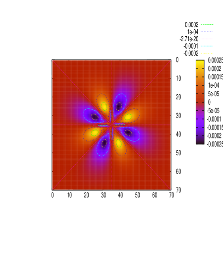
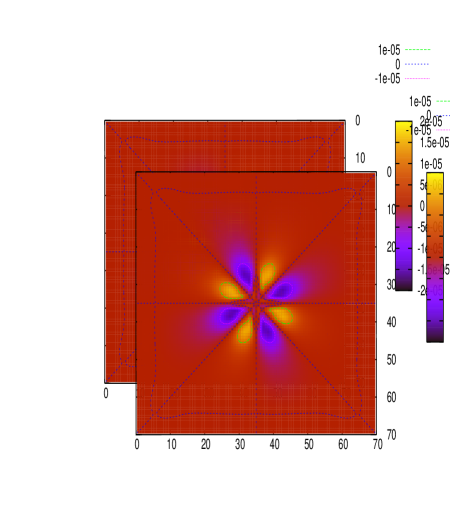
(a) Magnetic field	(b) Cross gradients of high order moments

Figure 12. Dimensionless magnetic field and cross gradients of high order moments (third and fifth) at $t\nu_{e,i}=8$.

The mecanism under consideration here (the magnetic field generation Figure 12), is expained in [23], as the results of non parallel gradients of the third and fifth moments of the electronic distribution function. We show the magnetic field in Figure 12,(a) and the cross gradients $\displaystyle\nabla_{\bf x}\left(\int_{\mathbb{R}^{3}}f_{e}\|{\bf v}\|^{3}d{\bf v}\right)\times\nabla_{\bf x}\left(\int_{\mathbb{R}^{3}}f_{e}\|{\bf v}\|^{5}d{\bf v}\right)$ in Figure 12,(b).
This mecanism is not due to the magnetic field generation from a $\nabla n_{e}\times\nabla T_{e}$ structure, since the density $n_{e}$ remains constant over the domain.
This structure with eight lobes is the result of the collision operators (of diffusion type) that make a particular speckle interact, after a rapid transient phase, with the other surrounding (similar) speckles. We note that an important parameter to anayse further such interactions should be the size of the speckle over the distance between speckles.

7. Conclusions

In the present paper, we have developed high order numerical methods dedicated to plasma simulation at a microscopic level.

A fourth order scheme issued from VFRoe schemes has been introduced in our kinetic context. It brings accuracy improvement on the velocity transport term. The second order scheme remains interesting for the linear spatial transport term (which is faced to less robustness and accuracy constraints) in a 2D, distributed memory context without overlapping between processors (each processor communicating with its neighbours only). It involves indeed a reduced stencil allowing for a lower minimum number of spatial grid points per processor.
The Maxwell equations have been discretized with a second order, implicit scheme allowing large time steps. We did not find any dependance on the Larmor radius and show that resolving the cyclotron frequency is sufficient. The couplings between the equations of the system have introduced a number of constraints (robustness, accuracy, symmetry) both on the transport scheme and the collision operators. Some numerical and physical test cases have validated our approach in different regimes of interest for ICF applications, and showed that it is computationally affordable. We also proposed a validation strategy in the linear regime based on [30], using Green kernels.
Various fundamental studies can be planned on the basis of the actual version of the solver. Collisional Weibel instability [28], forward and backward collisional Stimulated Brillouin Scattering, studies on the nonlocal interaction beween speckles for plasma-induced smoothing of laser beams issues [18], for instance. Also several axis of development are under consideration to bring more physics to the model: the ion motion, the extension to regimes relevant to higher laser intensities (relativistic regime and large angle collision terms of Boltzmann type).

Acknowledgments:

The authors are thankful to the Commissariat à l’Energie Atomique for the access to the CEA-CCRT-platine computing facillities. One of the author, Francis Filbet, would like to express his gratitude to the ANR JCJC-0136 MNEC (Méthode Numérique pour les Equations Cinétiques) funding.

Appendix A Electrostatic case in the linear regime

The relativistic $1D_{x}\times 3D_{\bf v}$Vlasov-Poisson system extracted from the equations (1)-(3) reads

(106) $$\frac{\partial f}{\partial t}+v_{1}\frac{\partial f}{\partial x_{1}}+\frac{q_{e}}{m_{e}}{E_{1}}\frac{\partial f}{\partial v_{1}}=0\ ,$$

(107) $$\frac{\partial E_{1}}{\partial x_{1}}=-\frac{q_{e}}{\epsilon_{0}}\left(n_{0}-\int_{\mathbb{R}^{3}}f(t,x_{1},{\bf v}){\bf dv}\right)\ .$$

The distribution function $f$ is assumed to be a perturbation around an equilibrium state $f^{(0)}(\|{\bf v}\|)$, $E^{(0)}_{1}=0$, $n_{0}=\displaystyle\int_{\mathbb{R}^{3}}f^{(0)}(\|{\bf v}\|){\bf d{v}}$. The system (106),(107) is linearized around this equilibrium state

(108) $$f(t,x_{1},{\bf v})=f^{(0)}(\|{\bf v}\|)+f^{(1)}(t,x_{1},{\bf v})\ ,$$

(109) $$E^{(1)}_{1}(t,x_{1})=E^{(0)}_{1}+E^{(1)}_{1}(t,x_{1})\ ,$$

under the hypothesis:

(110) $$\|f^{(1)}\|\ll\|f^{(0)}\|\ ,$$

(111) $$\|E^{(1)}_{1}\|\ll 1\ .$$

The Vlasov-Poisson can then be set under the following form (transport equation along the space directions supplemented by a source term along the $v_{1}$ direction), after linearization

(115) $$\left\{\begin{array}[]{ll}\displaystyle\frac{\partial f^{(1)}}{\partial t}+v_{1}\frac{\partial f^{(1)}}{\partial x_{1}}=-\frac{q_{e}}{m_{e}}E^{(1)}_{1}\frac{\partial f^{(0)}}{\partial v_{1}}\ ,\\ \\ \displaystyle\frac{\partial E^{(1)}_{1}}{\partial x_{1}}=\frac{q_{e}}{\epsilon_{0}}\int_{\mathbb{R}^{3}}f^{(1)}(t,x_{1},{\bf v}){\bf dv}\ .\end{array}\right.$$

If $f^{(1)}$ and $E^{(1)}_{1}$ are periodic and integrable, then their respective normalized Fourier coefficient are well-defined. A Fourier series expansion gives $\forall t>0$

(119) $$\left\{\begin{array}[]{ll}\displaystyle f^{(1)}(t,x_{1},{\bf v})=\hat{f}^{(1)}(t,k_{1},{\bf v})cos(k_{1}x_{1})\ ,\\ \\ \displaystyle\hat{f}^{(1)}(t,k_{1},{\bf v})=\frac{1}{L}\int_{0}^{L}f^{(1)}(t,x_{1},{\bf v})e^{-ik_{1}x_{1}}dx_{1}\ ,\end{array}\right.$$

Where $L$ is the size of the domain. The same reconstruction using Fourier series is used for $E^{(1)}_{1}$.
These coefficients verify the following equations,obtained by Fourier transformation performed on the equations of the system (115), for all real $k_{1}$

(120) $$\frac{\partial\hat{f}^{(1)}}{\partial t}+ik_{1}v_{1}\hat{f}^{(1)}=-\frac{q_{e}}{m_{e}}\hat{E}^{(1)}_{1}\frac{\partial f^{(0)}}{\partial v_{1}}\ ,$$

(121) $$ik_{1}\hat{E}_{1}=\frac{q_{e}}{\epsilon_{0}}\hat{n}_{1}\ .$$

Then introducing the notation $\hat{f}^{(1)}(t=0,k_{1},{\bf v})=\hat{f}^{(10)}(k_{1},{\bf v})$, the equation (120) can be written in the integral form

(122) $$\hat{f}^{(1)}(t,k_{1},{\bf v})=\hat{f}^{(10)}(k_{1},{\bf v})e^{-ik_{1}v_{1}t}-\frac{q_{e}}{m_{e}}\int_{0}^{t}\hat{E}^{(1)}_{1}(t^{\prime},k_{1})\frac{\partial f^{(0)}}{\partial v_{1}}e^{-ik_{1}v_{1}(t-t^{\prime})}dt^{\prime}\ .$$

Integrating the equation (122) over ${\bf v}$ and injecting in it the relation (121), one obtains the following integral equation for the density

(123) $$\hat{n}^{(1)}(t,k_{1})=M(t,k_{1})+\int^{t}_{0}K(t-t^{\prime},k_{1})\hat{n}^{(1)}(t^{\prime},k_{1})dt^{\prime}\ ,$$

where

(124) $$K(t,k_{1})=\frac{iq_{e}^{2}}{k_{1}m_{e}\epsilon_{0}}\int_{\mathbb{R}^{3}}\frac{\partial f^{(0)}}{\partial v_{1}}e^{-ik_{1}v_{1}t}{\bf d{v}}\ ,$$

(125) $$M(t,k_{1})=\int_{\mathbb{R}^{3}}\hat{f}^{(10)}(k_{1},{\bf v})e^{-ik_{1}v_{1}t}{\bf d{v}}\ .$$

These kernels can be computed with the desired accuracy, following [30]. The numerical resolution of (123) finally reduces to the inversion of a triangular linear system.
Macroscopic quantities such as the density or the heat flux can then be reconstructed using these latter equations.

Appendix B Initialisation for the generation of a single X-mode plasma wave

This test case stands as a validation for the couplings of Vlasov and Maxwell equations. We determine initial conditions that trigger a plasma wave at a given wavelength. To do so, Vlasov-Maxwell equations are linearized, setting $f=f^{(0)}+\tilde{f}$, $E=\tilde{E}$, $B=B^{(0)}+\tilde{B}$ around the equilibrium state $f=f^{(0)}$, $E=0$, $B=B^{(0)}$. In this appendix, we use the normalization (32)-(34). We assume periodic boundary conditions. The fluctuations of the total pressure tensor are neglected with respect to those of the magnetic field.
Using the conservation law $\displaystyle\frac{\partial n}{\partial t}+\frac{\partial j_{1}}{\partial{x_{1}}}=0$, the former hypothesis lead us to solve the system of six equations with six unknown $\tilde{j}_{1}$, $\tilde{j}_{2}$, $\tilde{E}_{1}$, $\tilde{E}_{2}$, $\tilde{B}_{3}$ and $\tilde{n}$

(126) $$\left\{\begin{array}[]{ll}\displaystyle\frac{\partial\tilde{j}_{1}}{\partial t}+\tilde{E}_{1}+B^{(0)}\tilde{j}_{2}=0\ ,\\ \displaystyle\frac{\partial\tilde{j}_{2}}{\partial t}+\tilde{E}_{2}-B^{(0)}\tilde{j}_{1}=0\ ,\\ \displaystyle\frac{\partial\tilde{n}}{\partial t}+\partial_{x_{1}}\tilde{j}_{1}=0\ ,\\ \displaystyle\frac{\partial\tilde{E}_{1}}{\partial x_{1}}=-\tilde{n}\ ,\\ \displaystyle\frac{\partial\tilde{E}_{2}}{\partial t}=-\frac{1}{\beta^{2}}\frac{\partial\tilde{B}_{3}}{\partial x_{1}}+\tilde{j}_{2}\ ,\\ \displaystyle\frac{\partial\tilde{B}_{3}}{\partial t}=-\frac{\partial\tilde{E}_{2}}{\partial x_{1}}\ .\end{array}\right.$$

Applying time and space Fourier tranform to this system, and identifying Fourier composants ($\tilde{n}=\hat{n}\exp(-i\omega t+ik_{1}x_{1})$), the following system is obtain

$$\left\{\begin{array}[]{ll}\displaystyle-i\omega\hat{j}_{1}+{\hat{E}}_{1}+B^{(0)}\hat{j}_{2}=0\ ,\\ \displaystyle-i\omega\hat{j}_{2}+\hat{E}_{2}-B^{(0)}\hat{j}_{1}=0\ ,\\ \displaystyle-i\omega\hat{n}+ik_{1}\hat{j}_{1}=0\ ,\\ \displaystyle ik_{1}\hat{E}_{1}=-{\hat{n}}\ ,\\ \displaystyle-i\omega\hat{E}_{2}=-\frac{1}{\beta^{2}}ik_{1}\hat{B}_{3}+\hat{j}_{2}\ ,\\ \displaystyle-i\omega\hat{B}_{3}=-ik_{1}\hat{E}_{2}\ .\end{array}\right.$$

The dispersion equation of this system reads

(127) $$N^{2}=\frac{k_{1}^{2}}{\beta^{2}\omega^{2}}=1-\frac{\omega^{2}-1}{\omega^{2}(\omega^{2}-1-\|B^{(0)}\|^{2})}\ .$$

In this equation, the plasma frequency is $\omega_{pe}=1$ and the cyclotron frequency is $\omega_{c}=q_{e}\|B^{(0)}\|/m$, that is $\|B^{0}\|$ in this dimensionless case. The perturbative term of the distribution function at initial time can be determined for a particular solution $\omega$ of this relation dispersion.
The Fourier transform is applied on the linearized Vlasov equation

(128) $$(-i\omega+ik_{1}v_{1})\hat{f}-\hat{E}_{1}\frac{\partial f^{(0)}}{\partial{v_{1}}}-\hat{E}_{2}\frac{\partial f^{(0)}}{\partial{v_{2}}}-B^{(0)}v_{2}\frac{\partial\hat{f}}{\partial{v_{1}}}+B^{(0)}v_{1}\frac{\partial\hat{f}}{\partial{v_{2}}}\,=\,0\ .$$

This equation is expressed in cylindrical coordinates

$$\left\{\begin{array}[]{ll}\displaystyle v_{1}=v_{\perp}\cos(\psi)\ ,\\ \displaystyle v_{2}=v_{\perp}\sin(\psi)\ ,\\ \displaystyle v_{3}=v_{\parallel}\end{array}\right.$$

where

$$\left\{\begin{array}[]{ll}\displaystyle v_{\perp}=(\|v_{1}\|^{2}+\|v_{2}\|^{2})^{1/2}\ ,\\ \displaystyle\tan(\psi)=\frac{v_{2}}{v_{1}}\ .\end{array}\right.$$

Recalling that:

$$\nabla_{\bf v}f=\frac{\partial f}{\partial v_{\perp}}\nabla_{\bf v}v_{\perp}+\frac{\partial f}{\partial\psi}\nabla_{\bf v}\psi+\frac{\partial f}{\partial v_{\parallel}}\nabla_{\bf v}v_{\parallel}\ ,$$

$$\left\{\begin{array}[]{ll}\displaystyle\frac{\partial v_{\perp}}{\partial v_{1}}=\cos(\psi)\ ,\\ \displaystyle\frac{\partial v_{\perp}}{\partial v_{2}}=\sin(\psi)\ ,\\ \displaystyle\frac{\partial\psi}{\partial v_{1}}=-\frac{1}{v_{\perp}}\sin(\psi)\\ \displaystyle\frac{\partial\psi}{\partial v_{2}}=\frac{1}{v_{\perp}}\cos(\psi)\ ,\end{array}\right.$$

with $\nabla_{\bf v}v_{\perp}=\vec{e}_{\perp}$, $\nabla_{\bf v}v_{\psi}=\vec{e}_{\psi}$ and $\nabla_{\bf v}v_{\parallel}=\vec{e}_{\parallel}$, where $\vec{e}$ are vectors in the local basis. Setting $f^{(0)}(\|{\bf v}\|^{2})=(2\pi)^{\frac{3}{2}}\exp(-\frac{\|{\bf v}\|^{2}}{2})$, and writing

$$({\bf v}\wedge{\bf B}).\nabla_{\bf v}\hat{f}=(\nabla_{\bf v}\hat{f}\wedge{\bf v}).{\bf B}=-B^{(0)}\frac{\partial f}{\partial\psi},\,\,\text{with}\,\,{\bf B}=(0,0,B^{(0)})\ ,$$

the kinetic equation (128) becomes

(129) $$(-i\omega+ik_{1}v_{\perp}\cos(\psi))\hat{f}+B^{(0)}\frac{\partial\hat{f}}{\partial\psi}+f^{(0)}(\|{\bf v}\|^{2})v_{\perp}(\hat{E}_{1}\cos(\psi)+\hat{E}_{2}\sin(\psi))=0.$$

In order to solve this equation, we decompose the distribution function as a Fourier serie

$$\hat{f}=\sum_{n=-\infty}^{+\infty}\hat{f}_{n}(v_{\perp})e^{in\psi}.$$

Then from (129),

$$\sum_{n=-\infty}^{+\infty}(-i\omega+ik_{1}v_{\perp}\cos(\psi)+inB^{(0)})\hat{f}_{n}e^{in\psi}=-f^{(0)}(\|{\bf v}\|^{2})v_{\perp}(\hat{E}_{1}\cos(\psi)+\hat{E}_{2}\sin(\psi))\ .$$

Multiplying this equation by $e^{im\psi}$, integrating from $0$ to $2\pi$, we obtain

$$\sum_{n=-\infty}^{+\infty}\int_{0}^{2\pi}e^{im\psi}(-i\omega+ik_{1}v_{\perp}\cos(\psi)+inB^{(0)})\hat{f}_{n}e^{in\psi}d\psi$$

(130) $$=-f^{(0)}(\|{\bf v}\|^{2})v_{\perp}\int_{0}^{2\pi}e^{im\psi}(\hat{E}_{1}\cos(\psi)+\hat{E}_{2}\sin(\psi))d\psi\ .$$

For $m=0$, terms are different from zero only for $n=-1,0,1$. From (B) comes

(131) $$k_{1}v_{\perp}\hat{f}_{-1}-2\omega\hat{f}_{0}+k_{1}v_{\perp}\hat{f}_{1}=0\ .$$

For $m=-1$,

(132) $$ik_{1}v_{\perp}\hat{f}_{0}-2i(\omega-B^{(0)})\hat{f}_{1}+ik_{1}v_{\perp}\hat{f}_{2}=-f_{0}(v^{2})v_{\perp}(\hat{E}_{1}-i\hat{E}_{2})\ .$$

For $m=1$,

(133) $$ik_{1}v_{\perp}\hat{f}_{-2}-2i(\omega+B^{(0)})\hat{f}_{-1}+ik_{1}v_{\perp}\hat{f}_{0}=-f^{(0)}(\|{\bf v}\|^{2})v_{\perp}(\hat{E}_{1}+i\hat{E}_{2})\ .$$

The case $m=-2$ involves $\hat{f}_{3}$,

(134) $$ik_{1}v_{\perp}\hat{f}_{1}-2(\omega-2B^{(0)})\hat{f}_{2}+ik_{1}v_{\perp}\hat{f}_{3}=0\ .$$

In the same manner the case $m=2$ involves $\hat{f}_{-3}$,

(135) $$ik_{1}v_{\perp}\hat{f}_{-3}-2(\omega+2B^{(0)})\hat{f}_{-2}+ik_{1}v_{\perp}\hat{f}_{-1}=0\ .$$

In order to close the system, the components $f_{-3}$ and $f_{3}$ are neglected, and we deduce from (131-135),

$$\left\{\begin{array}[]{rcl}-2(\omega+2B^{(0)})\hat{f}_{-2}+ik_{1}v_{\perp}\hat{f}_{-1}&=&0\ ,\\ ikv_{\perp}\hat{f}_{-2}-2i(\omega+B^{(0)})\hat{f}_{-1}+ik_{1}v_{\perp}\hat{f}_{0}&=&-f^{(0)}(\|{\bf v}\|^{2})v_{\perp}(\hat{E}_{1}+i\hat{E}_{2})\ ,\\ kv_{\perp}\hat{f}_{-1}-2\omega\hat{f}_{0}+k_{1}v_{\perp}\hat{f}_{1}&=&0\ ,\\ ik_{1}v_{\perp}\hat{f}_{0}-2i(\omega-B^{(0)})\hat{f}_{1}+ik_{1}v_{\perp}\hat{f}_{2}&=&-f^{(0)}(\|{\bf v}\|^{2})v_{\perp}(\hat{E}_{1}-i\hat{E}_{2})\ ,\\ ik_{1}v_{\perp}\hat{f}_{1}-2(\omega-2B^{(0)})\hat{f}_{2}&=&0\ .\end{array}\right.$$

The solution of linearized Vlasov equation can be calculted

$$\left\{\begin{array}[]{rcl}\displaystyle f(t,x,v)&=&f^{(0)}(\|{\bf v}\|^{2})+\sum_{n=-\infty}^{+\infty}\hat{f}_{n}(v_{\perp})e^{-i\omega t+ik_{1}x_{1}+in\psi}\ ,\\ \displaystyle E_{1}(t,x)&=&\hat{E}_{1}e^{-i\omega t+ik_{1}x_{1}}\ ,\\ \displaystyle E_{2}(t,x)&=&\hat{E}_{2}e^{-i\omega t+ik_{1}x_{1}}\ ,\\ \displaystyle B(t,x)&=&B^{(0)}+\hat{B}_{3}e^{-i\omega t+ik_{1}x_{1}}\ .\end{array}\right.$$

The dispersion relation (127) provides with a particular $\omega$. Then we obtain the following results for the construction of the initial solution,

$$f(0,x,v)=f^{(0)}(\|{\bf v}\|^{2})+\sum_{n=-2}^{2}\hat{f}_{n}(v_{\perp})e^{ik_{1}x+in\psi}$$

With the expressions

$$\begin{array}[]{rcl}\displaystyle\frac{\hat{f}_{-2}}{f^{(0)}(\|{\bf v}\|^{2})\hat{D}}&=&i(-4\,{\omega}^{3}{\hat{E}_{1}}-4\,i{\omega}^{3}{\hat{E}_{2}}+12\,i{\omega}^{2}{B^{(0)}}\,{\hat{E}_{2}}+12\,{\omega}^{2}{B^{(0)}}\,{\hat{E}_{1}}-8\,{{\|B^{(0)}\|}}^{2}\omega\,{\hat{E}_{1}}\\ \displaystyle\hfil&+&{k_{1}}^{2}{{v_{\perp}}}^{2}\omega\,{\hat{E}_{1}}+3\,i{k_{1}}^{2}{{v_{\perp}}}^{2}\omega\,{\hat{E}_{2}}-8\,i{{\|B^{(0)}\|}}^{2}\omega\,{\hat{E}_{2}}-4\,i{k_{1}}^{2}{{v_{\perp}}}^{2}{B^{(0)}}\,{\hat{E}_{2}}){{v_{\perp}}}^{2}k_{1},\\ \displaystyle\frac{\hat{f}_{-1}}{f^{(0)}(\|{\bf v}\|^{2})\hat{D}}&=&2\,i{v_{\perp}}\,({\hat{E}_{1}}\,{k_{1}}^{2}{{v_{\perp}}}^{2}{\omega}^{2}+4\,i{B^{(0)}}\,{\omega}^{3}{\hat{E}_{2}}-16\,{{\|B^{(0)}\|}}^{3}\omega\,{\hat{E}_{1}}-16\,i{{\|B^{(0)}\|}}^{3}\omega\,{\hat{E}_{2}}\\ \displaystyle\hfil&+&3\,i{\hat{E}_{2}}\,{k_{1}}^{2}{{v_{\perp}}}^{2}{\omega}^{2}-4\,{\hat{E}_{1}}\,{\omega}^{4}-8\,i{\hat{E}_{2}}\,{k_{1}}^{2}{{v_{\perp}}}^{2}{{\|B^{(0)}\|}}^{2}+2\,{k_{1}}^{2}{{v_{\perp}}}^{2}{B^{(0)}}\,\omega\,{\hat{E}_{1}}\\ \displaystyle\hfil&+&2\,i{k_{1}}^{2}{{v_{\perp}}}^{2}{B^{(0)}}\,\omega\,{\hat{E}_{2}}+16\,{\hat{E}_{1}}\,{{\|B^{(0)}\|}}^{2}{\omega}^{2}+16\,i{\hat{E}_{2}}\,{{\|B^{(0)}\|}}^{2}{\omega}^{2}+4\,{B^{(0)}}\,{\omega}^{3}{\hat{E}_{1}}\\ \displaystyle\hfil&-&4\,i{\hat{E}_{2}}\,{\omega}^{4}),\\ \displaystyle\frac{\hat{f}_{0}}{f^{(0)}(\|{\bf v}\|^{2})\hat{D}}&=&2\,i{{v_{\perp}}}^{2}k_{1}(16\,{{\|B^{(0)}\|}}^{2}\omega\,{\hat{E}_{1}}+{k_{1}}^{2}{{v_{\perp}}}^{2}\omega\,{\hat{E}_{1}}-4\,{\omega}^{3}{\hat{E}_{1}}+4\,i{\omega}^{2}{B^{(0)}}\,{\hat{E}_{2}}\\ \displaystyle\hfil&-&16\,i{{\|B^{(0)}\|}}^{3}{\hat{E}_{2}}+2\,i{k_{1}}^{2}{{v_{\perp}}}^{2}{B^{(0)}}\,{\hat{E}_{2}}),\\ \displaystyle\frac{\hat{f}_{1}}{f^{(0)}(\|{\bf v}\|^{2})\hat{D}}&=&2\,i(-2\,{B^{(0)}}+\omega){v_{\perp}}\,(-4\,i{k_{1}}^{2}{{v_{\perp}}}^{2}{B^{(0)}}\,{\hat{E}_{2}}+{k_{1}}^{2}{{v_{\perp}}}^{2}\omega\,{\hat{E}_{1}}-3\,i{k_{1}}^{2}{{v_{\perp}}}^{2}\omega\,{\hat{E}_{2}}\\ \displaystyle\hfil&-&12\,{\omega}^{2}{B^{(0)}}\,{\hat{E}_{1}}+12\,i{\omega}^{2}{B^{(0)}}\,{\hat{E}_{2}}-4\,{\omega}^{3}{\hat{E}_{1}}+4\,i{\omega}^{3}{\hat{E}_{2}}-8\,{{\|B^{(0)}\|}}^{2}\omega\,{\hat{E}_{1}}\\ \displaystyle\hfil&+&8\,i{{\|B^{(0)}\|}}^{2}\omega\,{\hat{E}_{2}}),\\ \displaystyle\frac{\hat{f}_{2}}{f^{(0)}(\|{\bf v}\|^{2})\hat{D}}&=&ik_{1}{{v_{\perp}}}^{2}(-4\,i{k_{1}}^{2}{{v_{\perp}}}^{2}{B^{(0)}}\,{\hat{E}_{2}}+{k_{1}}^{2}{{v_{\perp}}}^{2}\omega\,{\hat{E}_{1}}-3\,i{k_{1}}^{2}{{v_{\perp}}}^{2}\omega\,{\hat{E}_{2}}-12\,{\omega}^{2}{B^{(0)}}\,{\hat{E}_{1}}\\ \displaystyle\hfil&+&12\,i{\omega}^{2}{B^{(0)}}\,{\hat{E}_{2}}-4\,{\omega}^{3}{\hat{E}_{1}}+4\,i{\omega}^{3}{\hat{E}_{2}}-8\,{{\|B^{(0)}\|}}^{2}\omega\,{\hat{E}_{1}}+8\,i{{\|B^{(0)}\|}}^{2}\omega\,{\hat{E}_{2}}),\end{array}$$

where

$$\hat{D}=\omega\,(64\,{{\|B^{(0)}\|}}^{4}-16\,{k_{1}}^{2}{{v_{\perp}}}^{2}{\omega}^{2}+16\,{\omega}^{4}+16\,{k_{1}}^{2}{{v_{\perp}}}^{2}{{\|B^{(0)}\|}}^{2}+3\,{k_{1}}^{4}{{v_{\perp}}}^{4}-80\,{{\|B^{(0)}\|}}^{2}{\omega}^{2}).$$

$k_{1}v_{\perp}$ being small with respect to $B^{(0)}$ and $\omega$, powers of $k_{1}v_{\perp}$ can be neglected compared to these terms. The solution can be written

$$\begin{array}[]{rcl}\displaystyle\frac{\hat{f}_{-2}}{f^{(0)}(\|{\bf v}\|^{2})\hat{D}}&=&i{{v_{\perp}}}^{2}k_{1}(-4\,{\omega}^{3}{\hat{E}_{1}}-4\,i{\omega}^{3}{\hat{E}_{2}}+12\,i{\omega}^{2}{B^{(0)}}\,{\hat{E}_{2}}\\ \displaystyle\hfil&+&12\,{\omega}^{2}{B^{(0)}}\,{\hat{E}_{1}}-8\,{{\|B^{(0)}\|}}^{2}\omega\,{\hat{E}_{1}}-8\,i{{\|B^{(0)}\|}}^{2}\omega\,{\hat{E}_{2}}),\\ \displaystyle\frac{\hat{f}_{-1}}{f^{(0)}(\|{\bf v}\|^{2})\hat{D}}&=&2\,i{v_{\perp}}\,(4\,i{B^{(0)}}\,{\omega}^{3}{\hat{E}_{2}}-16\,{{\|B^{(0)}\|}}^{3}\omega\,{\hat{E}_{1}}-16\,i{{\|B^{(0)}\|}}^{3}\omega\,{\hat{E}_{2}}-4\,{\hat{E}_{1}}\,{\omega}^{4}\\ \displaystyle\hfil&+&16\,{\hat{E}_{1}}\,{{\|B^{(0)}\|}}^{2}{\omega}^{2}+16\,i{\hat{E}_{2}}\,{{\|B^{(0)}\|}}^{2}{\omega}^{2}+4\,{B^{(0)}}\,{\omega}^{3}{\hat{E}_{1}}-4\,i{\hat{E}_{2}}\,{\omega}^{4}),\\ \displaystyle\frac{\hat{f}_{0}}{f^{(0)}(\|{\bf v}\|^{2})\hat{D}}&=&2\,i{{v_{\perp}}}^{2}k_{1}(16\,{{\|B^{(0)}\|}}^{2}\omega\,{\hat{E}_{1}}+{k_{1}}^{2}{{v_{\perp}}}^{2}\omega\,{\hat{E}_{1}}-4\,{\omega}^{3}{\hat{E}_{1}}+4\,i{\omega}^{2}{B^{(0)}}\,{\hat{E}_{2}}\\ \displaystyle\hfil&-&16\,i{{\|B^{(0)}\|}}^{3}{\hat{E}_{2}}),\\ \displaystyle\frac{\hat{f}_{1}}{f^{(0)}(\|{\bf v}\|^{2})\hat{D}}&=&2\,i{v_{\perp}}\,(\omega-2\,{B^{(0)}})(-12\,{\omega}^{2}{B^{(0)}}\,{\hat{E}_{1}}+12\,i{\omega}^{2}{B^{(0)}}\,{\hat{E}_{2}}-4\,{\omega}^{3}{\hat{E}_{1}}+4\,i{\omega}^{3}{\hat{E}_{2}}\\ \displaystyle\hfil&-&8\,{{\|B^{(0)}\|}}^{2}\omega\,{\hat{E}_{1}}+8\,i{{\|B^{(0)}\|}}^{2}\omega\,{\hat{E}_{2}}),\\ \displaystyle\frac{\hat{f}_{2}}{f^{(0)}(\|{\bf v}\|^{2})\hat{D}}&=&ik_{1}{{v_{\perp}}}^{2}(-12\,{\omega}^{2}{B^{(0))}}\,{\hat{E}_{1}}+12\,i{\omega}^{2}{B^{(0)}}\,{\hat{E}_{2}}-4\,{\omega}^{3}{\hat{E}_{1}}+4\,i{\omega}^{3}{\hat{E}_{2}}\\ \displaystyle\hfil&-&8\,{{\|B^{(0)}\|}}^{2}\omega\,{\hat{E}_{1}}+8\,i{{\|B^{(0)}\|}}^{2}\omega\,{\hat{E}_{2}}),\end{array}$$

where

$$\hat{D}=\omega\,(64\,{{\|B^{(0)}\|}}^{4}+16\,{\omega}^{4}-80\,{{\|B^{(0)}\|}}^{2}{\omega}^{2}).$$

We choose to initialise the perturbation from the amplitude of the magnetic field:

$$\hat{B}_{3}=A\text{ where }A\in[0,1].$$

Then from the system (126) and the dispersion relation (127), we deduce the values of $\hat{E}_{1}$, $\hat{E}_{2}$ and thus reconstruct the $\hat{f}_{i}$,

$$\hat{E}_{1}={\frac{-i{\hat{B}_{3}}\,\left({\omega}^{4}{\beta}^{2}-{\omega}^{2}{k_{1}}^{2}-{\omega}^{2}{\beta}^{2}-{{\|B^{(0)}\|}}^{2}{\omega}^{2}{\beta}^{2}+{{\|B^{(0)}\|}}^{2}{k_{1}}^{2}\right)}{k_{1}{\beta}^{2}{B^{(0)}}}},\,\,\,\hat{E}_{2}=\frac{\omega\hat{B}_{3}}{k_{1}}.$$

References

• [1] F. Alouani-Bibi, M.M. Shoucri, J.-P. Matte Different Fokker-Planck approaches to simulate electron transport in plasmas Computer Physics Communication, 164, 60-66, 2004.
• [2] R. Balescu, Transport processes in plasmas vol.1 classical transport theory, 1988
• [3] A.R. Bell, A.P.L. Robinson, M. Sherlock, R.J. Kingham and W. Rozmus Fast electron transport in laser-produced plasmas and the KALOS code for solution of the Vlasov-Fokker-Planck equation, Plasma Physics and controlled fusion, 48, R37-R57, 2006.
• [4] D. Bennaceur-Doumaz, A. Bendib, Nonlocal electron transport in magnetized plasmas with arbitrary atomic number, Physics of Plasmas, 13, 092308, 2006
• [5] C. Berthon and F. Marche Accepted in SIAM J. SCI. COMP.
• [6] S. I. Braginskii, Rewiews of plasma physics, Consultants Bureau, New York, 1965, Vol.1, p.205
• [7] A. Bret, M.-C. Firpo, C. Deutsch Characterization of the Initial Filamentation of a Relativistic Electron Beam Passing through a Plasma, Physical Review Letters, 94, 115002, 2005.
• [8] A. Bret, L. Gremillet, D. Bénisti, E. Lefebvre Exact Relativistic Kinetic Theory of an Electron-beam-Plasma System: Hierarchy of the Competing Modes in the system-Parameter Space, Physical Review Letters, 100, 205008, 2008.
• [9] C. Buet, S. Cordier, Numerical analysis of conservative and entropy schemes for the Fokker-Planck-Landau equation , Numer. Anal. 36 (1999) 953-973.
• [10] C. Buet, S. Cordier, P. Degong, M. Lemou, Fast algorithm for numerical, conservative and entropy approximation of the Fokker-Planck-Landau equation , J. Comput. Physics 133 (1997) 310-322.
• [11] C. Buet, S. Cordier, F. Filbet, Comparison of numerical scheme for Fokker-Planck-Landau equation , ESAIM Proc. 10 (1999) 161-181.
• [12] N. Crouseilles, F. Filbet, Numerical approximation of collisional plasmas by high order methods, Journal of Computational Physics, 201, 546-572, 2004.
• [13] A. Decoster, P.A. Markowich, B. Perthame, Modeling of collisions, Research in applied mathematics, Masson, Paris, 1997.
• [14] P. Degond, B. Lucquin-Desreux, An entropy scheme for the Fokker-Planck collision operator of plasma kinetic theory, Numer. Math. 68 (1994) 239-262
• [15] B. Dubroca, M. Tchong, P. Charrier, V.T. Tikhonchuk, J.P. Morreeuw Magnetic field generation in plasmas due to anisotropic laser heating, Phys. Plasma, 11, 3830, 2004.
• [16] E. M. Epperlein, M. G. Haines, Plasma transport coefficients in a magnetic field by direct numerical solution of the Fokker-Planck equation, Phys. Fluids 29 (4), April 1986
• [17] E. M. Epperlein, Kinetic theory of laser filamentation in plasmas, Phys. Rew. Letter 65, 2145, 1990.
• [18] J.-L. Feugeas, Ph Nicolai, X. Ribeire, G. Schurtz, V. Tikhonchuk and M. Grech, Modelling of two dimensional effects in hot spot relaxation in laser-produced plasmas, Physics of Plasmas, 15, 062701, 2008.
• [19] F. Filbet, L. Pareshi Numerical method for the accurate solution of the Fokker-Planck-Landau equation in the non-homogeneous case, Journal of Computational Physics, 179, 1-26, 2002.
• [20] F. Filbet, E. Sonnendrücker, Comparison of Eulerian Vlasov solvers, Computer Physics Communications, 150, 3, pp. 247-266(20), 2003.
• [21] M.G. Haines Magnetic-field generation in laser fusion and hot-electron transport, Can. J. Phys., 64, 912, 1986.
• [22] R.J. Kingham, A.R. Bell An implicit Vlasov-Fokker-Planck code to model non-local electron transport in 2-D with magnetic fields Journal of Computational Physics, 194, 1-34, 2004.
• [23] R.J. Kingham, A.R. Bell, Nonlocal Magnetic-Field Generation in Plasmas without Density Gradients, Phys. Rew. Letter, 88, 045004, 2002.
• [24] A. Kurganov, E. Tadmor, Solution of Two-Dimensional Riemann Problems for Gas Dynamics without Riemann Problem Solvers, Numerical methods Partial Differential, 218, 584-608, 2002.
• [25] S. Le Bourdiec, F. de Vuyst, L. Jacquet, Numerical solution of the Vlasov-Poisson system using generalized Hermite functions, Computer Physics Communications 175 (2006) 528-544
• [26] M. Lemou Multipole expansions for the Fokker-Planck-Landau operator, Numer. Math., 78, 597-618, 1998
• [27] L. Pareshi, G. Russo, G. Toscani, Fast spectral method for Fokker-Planck-Landau collision operator , J. Comput. Physics 165 (2000) 216-236.
• [28] A. Sangam, J.-P. Morreeuw, V.T. Tikhonchuk Anisotropic instability in a laser heated plasma, Phys. Plasmas 14, 053111 (2007)
• [29] J.J. Santos et al. Fast-electron transport and induced heating in aluminium foils, Physics of Plasmas, 14, 103107, 2007.
• [30] C. Sartori et G.G M. Coppa, Analysis of transient and asymptotic behavior in relativistic Landau damping, Phys. Plasmas 2 (11), 1995.
• [31] V.K. Senecha, A.V. Brantov, V. Yu Bychenkov, V.T. Tikhonchuk Temperature relaxation in hot spots in a laser-produced plasma, Phys. Review E, 47, 1, 1998.
• [32] Y. Sentoku, A.J. Kemp Numerical method for particle simulations at extreme densities and temperatures: Weighted particles, relativistic collisions and reduced currents, Article in Press, Journal of Computational Physics, April (2008).
• [33] M. Tabak et al. Ignition and high gain with ultrapowerful lasers, Physics of Plasmas 1, 1626, 1994.
• [34] B. Van Leer Towards the ultimate conservative difference scheme. V. A second-order sequel to Godunov’s method, J. Comput. Phys., 32, 101-136 (1979)
• [35] S. Yamamoto, H. Daiguji High order accurate upwind schemes for solving the compressible Euler and Navier-Stokes equations, Computers Fluids, 22, 259-270 (1993)
• [36] T. Yokota, Y. Nakao, T. Johzaki, K. Mima Two-dimensional relativistic Fokker-Planck model for core plasma heating in fast ignition targets, Physics of Plasmas, 13, 022702, 2006.