Next-to-leading order static gluon self-energy for anisotropic plasmas
M.E. Carrington
Brandon University,
Brandon, Manitoba, R7A 6A9 Canada
and Winnipeg Institute for Theoretical Physics,
Winnipeg, Manitoba, Canada
A. Rebhan
Institut für Theoretische Physik, Technische Universität Wien, Wiedner Hauptstraße 8-10, A-1040 Vienna, Austria
Abstract
In this paper the structure of the next-to-leading (NLO) static gluon self energy for an anisotropic plasma is investigated in the limit of a small momentum space anisotropy. Using the Ward identities for the static hard-loop (HL) gluon polarization tensor and the (nontrivial) static HL vertices, we derive a comparatively compact form for the complete NLO correction to the structure function containing the space-like pole associated with magnetic instabilities. On the basis of a calculation without HL vertices, it has been conjectured that the imaginary part of this structure function is nonzero, rendering the space-like poles integrable. We show that there are both positive and negative contributions when HL vertices are included, highlighting the necessity of a complete numerical evaluation, for which the present work provides the basis.
pacs:
11.10Wx, 11.15Bt, 12.38Mh
††preprint: TUW-08-18
I Introduction
The difficulties in explaining the strong collective phenomena observed at the Relativistic Heavy Ion collider (RHIC) Tannenbaum:2006ch by perturbative QCD at finite temperature have led to extensive studies of the consequences of the inevitable presence of non-Abelian plasma instabilities Mrowczynski:1988dz ; Pokrovsky:1988bm ; Mrowczynski:1993qm in a plasma with momentum-space anisotropy. To leading order in the coupling and for small gauge field amplitudes, the dynamics of plasma instabilities are determined by the generalization of the hard-thermal-loop (HTL) Weldon:1982aq ; Frenkel:1990br ; Braaten:1990mz gauge boson self-energy to anisotropic situations Mrowczynski:2000ed ; Romatschke:2003ms ; Romatschke:2004jh ; Arnold:2003rq .
In equilibrium, it is well known that non-bilinear terms in the HTL effective action Taylor:1990ia ; Braaten:1992gm are important at next-to-leading order (NLO). In order to obtain complete NLO corrections to HTL dispersion laws such as plasmon damping constants, one must resum both propagators and vertices Braaten:1990it ; Braaten:1992gd ; Kobes:1992ys ; Schulz:1994gf ; Carrington:2006gb ; Carrington:2008dw . In anisotropic systems, the non-bilinear terms in the corresponding hard-loop (HL) effective action Mrowczynski:2004kv are important for the dynamics of non-Abelian plasma instabilities at large gauge field amplitudes, which has been studied using real-time lattice simulations Rebhan:2004ur ; Arnold:2005vb ; Rebhan:2005re ; Bodeker:2007fw ; Arnold:2007cg ; Rebhan:2008uj . Up to now, analytic calculations at NLO in anisotropic systems have been considered prohibitively difficult. In addition to the obvious technical difficulties associated in dealing with expressions that contain huge numbers of terms, these calculations contain new conceptual problems arising from the fact that the anisotropic gluon propagator contains non-integrable space-like poles.
In perturbative estimates of jet quenching and momentum broadening in the anisotropic quark-gluon plasma, such non-integrable singularities also appear Romatschke:2006bb ; Baier:2008js . It has been suggested in Romatschke:2006bb that the static gluon self energy might develop a non-zero imaginary part at NLO that regulates these singularities. In thermal equilibrium, the imaginary part of the static gluon self energy, which is an odd function of the frequency, vanishes due to the KMS condition LeB:TFT . In the anisotropic case, it seems possible that there is a finite, discontinuous contribution.
Ref. Romatschke:2006bb provided support for this conjecture in the form of a partial calculation of the anisotropic NLO static gluon self-energy. This calculation included however only a tadpole diagram with a bare four-vertex.
In this paper, we provide the basis for a complete analytic calculation of the anisotropic NLO static gluon self-energy. In the HTL case, only static loop momenta have to be considered, no fermion loops contribute, and all HTL vertex corrections vanish Rebhan:1993az . However, the anisotropic HL vertex corrections do not vanish in the static limit Mrowczynski:2004kv .
The relevant diagrams are shown in Fig. 1 (since the ghost self energy vanishes at leading order, the ghosts do not need to be resummed). The solid dots indicate leading order propagators and vertices which are obtained from the hard loop (HL) effective action Mrowczynski:2004kv . The third diagram is the HL counterterm which must be subtracted to avoid double counting.
In this paper, we give an analytic result for the integrand corresponding to the diagrams in Fig. 1. After extensive algebraic manipulations, the final expression has a relatively simple form, because of cancellations that occur between different contributions from the tadpole and bubble contributions. We divide the result into ‘tadpole-like’ contributions (which contain only one HL propagator) and ‘bubble-like’ contributions (which contain two HL propagators).
We calculate the contribution from ‘tadpole-like’ contributions with a bare vertex. We compare our result with the (corrected) result of Romatschke:2006bb for the tadpole diagram (without taking into account cancellations with the bubble diagram) with a bare vertex.
Figure 1: The diagrams that contribute to static gluon self energy. All lines correspond to gluon propagators. The dots indicate hard loop propagators and vertices. The cross denotes the HL counterterm.
II Notation and hard anisotropic loops
In this section we define our notation for the anisotropic HL quantities
and give the explicit form of the static HL propagator in Feynman gauge.
At zero temperature, field theory can be formulated covariantly. At finite temperature, covariance is broken by the vector which specifies the rest frame of the thermal system. For anisotropic systems we need (in the simplest case) one additional vector to specify the direction of the anisotropy. We consider the case in which there is one preferred spatial direction along which the system is anisotropic (in planes transverse to this vector the system is isotropic). In the context of heavy ion collisions, we can take this direction to be the beam axis () along which the initial expansion occurs.
II.1 Distribution Functions
We define the isotropic particle distribution:
(1)
In equilibrium, we have
(2)
We define the Debye mass from the equilibrium distribution111footnotetext: In Ref. Romatschke:2003ms ; Romatschke:2004jh Eq. (3) differs by a factor of 2 and Eq. (1) differs by a factor 1/2. The definition of the Debye mass is the same.
(3)
Following Romatschke:2003ms ; Romatschke:2004jh , we can construct an anisotropic distribution from any isotropic distribution of the form by writing
(4)
where is the anisotropy parameter. A value corresponds to a contraction of the distribution and corresponds to a stretching of the distribution. In this paper we restrict ourselves to weakly anisotropic systems for which .
which satisfies .
Throughout this paper we will frequently use the indices to denote momentum arguments. For example: we will write . We also use Latin letters to denote spatial indices, with the exception that the indices , , are reserved and used exclusively to denote momenta. Using the vector in (5), we construct the projection operators:
(6)
which satisfy:
(7)
II.3 Lowest Order Self Energy
We define the polarization tensor using the relation:
(8)
The HL gluon self energy is gauge invariant and satisfies the usual Ward identity: . Consequently, we only need to calculate the spatial components. At finite temperature, there are two independent components which are called the transverse and longitudinal parts. For anisotropic systems the self energy can be decomposed into four independent structure functions:
We calculate the static propagator in the covariant gauge (with Feynman gauge parameter) by inverting (8).
This inversion is complicated by the fact that the anisotropic propagator depends on the two fixed vectors (1,0,0,0) and (0,0,0,1), as well as the 4-momentum . The method is described in Kobes:1991dc . The result is:
(13)
In the small- limit, the result (11) implies that has a pole at negative which corresponds to the usual electric (Debye) screening. For non-vanishing space-like poles also appear. Writing , and we find that these space-like poles appear at:
(14)
When is positive, corresponding to an oblate particle distribution, has a space-like pole for and . For negative, the space-like pole occurs for . has a space-like pole for any positive value of unless . These poles of correspond to the magnetic Weibel instability Weibel:1959 .
II.5 Vertices
In this section we give our notation for the HL vertices Mrowczynski:2004kv . We define:
(15)
The 2-point function is:
(16)
The 3-point function is222footnotetext: In Ref. Mrowczynski:2004kv there is a missing factor (-1) in Eq. (35)
(17)
The 4-point function is333footnotetext: In Ref. Mrowczynski:2004kv there is a missing factor (-1/2) in Eq. (39) and a missing in Eq. (38)
(18)
Momenta are taken to be incoming. When the momentum arguments are not written explicitly, they are taken to be in the order for the 3-point function and for the 4-point function.
The HL vertices satisfy the Ward identities:
(19)
The tadpole form of the 4-point vertex has a simpler form:
(20)
This vertex satisfies the Ward identities:
(21)
We also define the bare vertices:
(22)
Using these definitions we write the integrand corresponding to the first two diagrams in Fig. 1 as:
(23)
The order of the momentum variables is for the 3-point functions and for the 4-point functions.
Eq. (23) is to be understood as restricted to the static case
and small momentum anisotropy such that the prefactor of the integral is simply the
temperature of the isotropic distribution function (2).
III Integrand for
We calculate the NLO contribution to which is obtained from (10) as:
(24)
with as given in (23).
The resulting integrand can be rewritten in a comparatively compact form. The method is similar to the calculations of the integrands that give the NLO equilibrium gauge boson polarization Braaten:1990it , and the NLO equilibrium fermion self energy Braaten:1992gd ; Kobes:1992ys ; Carrington:2006gb . The basic procedure is as follows. We substitute the static propagator as given in Eq. (13). Then we use the Ward identities in Eqs. (19) and (21). This produces factors proportional to components of the HL polarization tensor in the numerator. These factors can be expressed as pieces of inverse propagators, which cancel with the corresponding components of the original propagators. This procedure allows us to identify cancellations between various pieces of the first two diagrams shown in Fig. 1. We divide the result into several types of contributions: (i) terms in which all factors of the HL propagator have cancelled; (ii) tadpole-like terms which contain only one propagator; (iii) bubble-like terms that contain two propagators and no HL vertices; (iv) bubble-like terms that contain two propagators and one HL vertex; and (v) bubble-like terms that contain two propagators and two HL vertices. We thus write
(25)
where the result for the various contributions to the integrand are given below.
To compactify the expression we use the notation:
(26)
The separate integrands then read:
(i) terms in which all factors of the HL propagator have cancelled:
(27)
(ii) tadpole-like terms:
(iii) bubble-like terms with no HL vertices:
(iv) bubble-like terms with one HL vertex:
(v) bubble-like terms with two HL vertices:
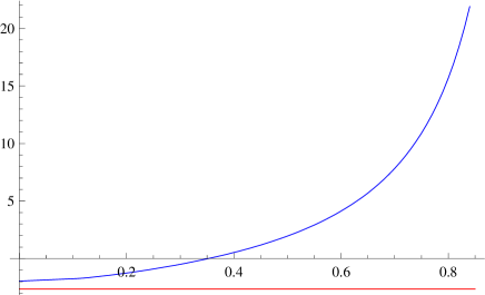
IV Imaginary part of tadpole-like terms
We have evaluated numerically the imaginary part of the tadpole-like terms given in (III) with the HL vertices set to zero. The result is
given in Fig. 2.
We compare with the result of Romatschke:2006bb for the tadpole diagram with a HL propagator and a bare vertex (see Appendix A):
(32)
Figure 2: (Color online) The result for as a function of for the simple tadpole (the (red) straight line) as given in Eq. (32), and for the ‘full’-tadpole (the (blue) curve) as given in Eq. (III). The factor has been extracted.
By considering only the tadpole diagram with a HL propagator but a bare vertex,
Ref. Romatschke:2006bb has obtained an imaginary part Im
which is of the order and strictly negative.
Our result, which includes also contributions from the bubble diagram
with HL vertices where the latter have cancelled one of the two HL propagators,
shows that this finding is not generic as far as the sign of the result is
concerned. Evidently, the complete static NLO gauge boson self energy contains
positive as well as negative contributions to the imaginary part, and
it remains to be seen whether a complete numerical evaluation of the
expressions that we have presented here will lead to a nonzero result.
V Conclusions
The main result of this paper is a relatively simple result for the integrand that gives the complete NLO contribution to the component of the gluon self energy, in the static limit. We have calculated analytically the contribution to the imaginary part from ‘tadpole-like’ terms, by which we mean contributions which involve only a single HL propagator after Ward identities have been used to reduce the diagram involving two HL propagators and two HL 3-vertices. The result is of the order predicted in Romatschke:2006bb , but the tadpole-like contribution is not strictly negative.
Indeed, from previous experience with equilibrium hard thermal loop calculations, one would expect cancellations between the various contributions to the full integral. For the equilibrium case, the KMS conditions actually guarantee that the imaginary part of the self energy is zero in the static limit, at all orders. Out of equilibrium, the result must be odd in the frequency, which means that any nonzero result must contain a discontinuity at vanishing frequency. The existence of this discontinuity at
the order has been conjectured in Romatschke:2006bb and
used for a perturbative estimate of the order of magnitude of
jet quenching and momentum broadening parameters
Romatschke:2006bb ; Baier:2008js .
In order to determine whether there is in fact a non-zero contribution to the imaginary part of the complete static gluon self-energy at next-to-leading, the full integral, as given in Eqs. (III)–(III), must be evaluated numerically. This calculation, which involves some nested integrations with highly nontrivial
integrands, is in progress.
In this Appendix we point out a few errors that occurred in
the calculation of the tadpole diagram with bare vertex which was
presented in the Appendix of Ref. Romatschke:2006bb . The main mistake is the incorrect
assumption 111We thank Paul Romatschke for discussions of this point. of a relation of the form
which leads to the incorrect simplification:
(33)
(34)
However, the results given in Ref. Romatschke:2006bb do not satisfy (34) because of typographical errors.
We write below the results from Romatschke:2006bb for and from Eq. (A3) of that paper, with an extra factor in front of the logs, and an extra factor (-1) in front of the result for . These extra factors are written in square brackets.
(35)
These ‘adjusted’ expressions satisfy Eq. (34). However Eq. (33) is not valid (not even at leading order).
References
(1)
M. J. Tannenbaum, Rept. Prog. Phys. 69, 2005 (2006).
(2)
S. Mrówczyński, Phys. Lett. B214, 587 (1988).
(3)
Y. E. Pokrovsky and A. V. Selikhov, JETP Lett. 47, 12 (1988).
(4)
S. Mrówczyński, Phys. Lett. B314, 118 (1993).
(5)
H. A. Weldon, Phys. Rev. D26, 1394 (1982).
(6)
J. Frenkel and J. C. Taylor, Nucl. Phys. B334, 199 (1990).
(7)
E. Braaten and R. D. Pisarski, Nucl. Phys. B337, 569 (1990).
(8)
S. Mrówczyński and M. H. Thoma, Phys. Rev. D62, 036011 (2000).
(9)
P. Romatschke and M. Strickland, Phys. Rev. D68, 036004 (2003).
(10)
P. Romatschke and M. Strickland, Phys. Rev. D70, 116006 (2004).
(11)
P. Arnold, J. Lenaghan, and G. D. Moore, JHEP 08, 002 (2003).
(12)
J. C. Taylor and S. M. H. Wong, Nucl. Phys. B346, 115 (1990).
(13)
E. Braaten and R. D. Pisarski, Phys. Rev. D45, 1827 (1992).
(14)
E. Braaten and R. D. Pisarski, Phys. Rev. D42, 2156 (1990).
(15)
E. Braaten and R. D. Pisarski, Phys. Rev. D46, 1829 (1992).
(16)
R. Kobes, G. Kunstatter, and K. Mak, Phys. Rev. D45, 4632 (1992).
(17)
H. Schulz, Nucl. Phys. B413, 353 (1994).
(18)
M. E. Carrington, Phys. Rev. D75, 045019 (2007).
(19)
M. E. Carrington, A. Gynther, and D. Pickering, Phys. Rev. D78, 045018
(2008).
(20)
S. Mrówczyński, A. Rebhan, and M. Strickland, Phys. Rev. D70,
025004 (2004).
(21)
A. Rebhan, P. Romatschke, and M. Strickland, Phys. Rev. Lett. 94, 102303
(2005).
(22)
P. Arnold, G. D. Moore, and L. G. Yaffe, Phys. Rev. D72, 054003 (2005).
(23)
A. Rebhan, P. Romatschke, and M. Strickland, JHEP 0509, 041 (2005).
(24)
D. Bödeker and K. Rummukainen, JHEP 07, 022 (2007).
(25)
P. Arnold and G. D. Moore, Phys. Rev. D76, 045009 (2007).
(26)
A. Rebhan, M. Strickland, and M. Attems, Phys. Rev. D78, 045023 (2008).
(27)
P. Romatschke, Phys. Rev. C75, 014901 (2007).
(28)
R. Baier and Y. Mehtar-Tani, Jet quenching and broadening: the transport
coefficient in an anisotropic plasma, arXiv:0806.0954, 2008.
(29)
M. Le Bellac, Thermal Field Theory (Cambridge University Press,
Cambridge, UK, 1996).
(30)
A. K. Rebhan, Phys. Rev. D48, 3967 (1993).
(31)
R. Kobes, G. Kunstatter, and A. Rebhan, Nucl. Phys. B355, 1 (1991).