Analysis of Firing Behaviors in Networks of Pulse-Coupled Oscillators
with Delayed Excitatory Coupling

Abstract

For networks of pulse-coupled oscillators with delayed excitatory coupling, we analyze the firing behaviors depending on coupling strength and transmission delay. The parameter space consisting of strength and delay is partitioned into two regions. For one region, we derive a low bound of interspike intervals, from which three firing properties are obtained. However, this bound and these properties would no longer hold for another region. Finally, we show the different synchronization behaviors for networks with parameters in the two regions.

For decades, complex networks have been focused on by scientists from various fields, for instance, sociology, biology, chemistry and physics, etc. In particular, networks of pulse-coupled oscillators, as an important class of interconnected dynamical systems, have gained increasing attentions because of their intimate relationship to natural systems as diverse as cardiac pacemaker cells, flashing fireflies, chirping crickets, biological neural networks, and earthquakes (cf. relationship-to-natual-systems ; Buck1988 ; Mirollo1990 ). A pioneering work on modeling and analyzing pulse-coupled units was done by Mirollo and Strogatz Mirollo1990 . Inspired by Peskin’s model for self-synchronization of the cardiac pacemaker, they proposed a pulse-coupled oscillator model with undelayed excitatory coupling to explain the synchronization of huge congregations of South East Asian fireflies. With the framework of the Mirollo-Strogatz model, many theoretical and numerical results on pulse-coupled networks have been obtained Vreeswijk1993-Chen1994-Corral1995 ; Mathar1996-Goel2002 ; Ernst1995 ; Ernst1998 ; Timme2002-1 ; Timme2002-2 ; Kim2004 ; Wu2007 .

Pulse-coupling is difficult to handle mathematically because it introduces discontinuous behavior into the otherwise continuous model and so stymies most of the standard mathematical techniques Strogatz1983 . Particularly for delayed pulse-coupling, the mathematical analysis of collective dynamics of networks becomes a challenging problem. Past research experience indicates that some underlying facts and assumptions about firing behaviors play a crucial role in mathematical analysis Mirollo1990 ; Mathar1996-Goel2002 ; Ernst1995 ; Ernst1998 ; Timme2002-1 ; Timme2002-2 ; Wu2007 . For example, in Mirollo1990 ; Mathar1996-Goel2002 , synchronization was proved by making use of the fact that the firing order of oscillators is always preserved for complete and undelayed pulse-coupling; in Ernst1998 , an assumption about firing times made the analysis easier by reducing the number of case distinctions; in Wu2007 , the proof of desynchronization was essentially due to a low bound of interspike intervals.

In this Letter, networks of pulse-coupled oscillators with delayed excitatory coupling are studied. We analyze the firing behaviors depending on coupling strength and transmission delay. The parameter space consisting of strength and delay is partitioned into two regions. For one region, we give a low bound of interspike intervals. By using the bound, three firing properties are derived, which would be very helpful for discussing synchronization of networks and stability of periodic solutions. Unfortunately, these properties no longer hold for another region. Furthermore, the different synchronization behaviors for networks with parameters in the two regions are presented.

We consider a system of $N$ identical oscillators which are pulse-coupled in a delayed excitatory manner. As in Timme2002-1 , the coupling structure is specified by the sets $\mathrm{Pre}(i)$ of presynaptic oscillators that send pulses to oscillator $i$, or the sets $\mathrm{Post}(i)$ of postsynaptic oscillators that receive pulses from oscillator $i$. A phase variable $\phi_{i}(t)\in[0,1]$ is used to characterize the state of the oscillator $i$ at time $t$. In the case of no interaction, the dynamics of $\phi_{i}$ is given by

$$\mathrm{d}\phi_{i}(t)/\mathrm{d}t=1,$$ (1)

namely, the cycle period of the free oscillator is 1. When $\phi_{i}$ reaches the threshold $\phi_{i}=1$, the oscillator $i$ fires and $\phi_{i}$ jumps back instantly to zero, after which the cycle repeats. That is,

$$\phi_{i}(t)=1\Rightarrow\phi_{i}(t^{+})=0.$$ (2)

Because of the transmission delay, the oscillators interact by the following form of pulse-coupling: if oscillator $i$ fires at time $t$, it emits a spike instantly; after a delay time $\tau$, the spike reaches all postsynaptic oscillators $j\in\mathrm{Post}(i)$ and induces a phase jump according to

$$\phi_{j}(t+\tau)=f^{-1}(\min[1,f(\phi_{j}((t+\tau)^{-}))+\varepsilon_{ij}]),$$ (3)

where $\varepsilon_{ij}>0$ is the coupling strength from oscillator $i$ to oscillator $j$; and the function $f$ is twice continuously differentiable, monotonously increasing, $f^{\prime}>0$, concave down, $f^{\prime\prime}<0$, and satisfies $f(0)=0$, $f(1)=1$. For a more detailed introduction of the model, see Mirollo1990 ; Ernst1995 ; Ernst1998 ; Timme2002-1 ; Timme2002-2 ; Wu2007 . In this Letter, we further assume the following: (i) The coupled system starts at time $t=0$ with a set of initial phases $0<\phi_{i}(0)\leq 1$; (ii) there is no self-interaction, i.e., $i\not\in\mathrm{Pre}(i)$ for any oscillator $i$; (iii) $0<\tau<1$; and (iv) the coupling strengths are normalized such that for all oscillator $i$, $\sum_{j\in\mathrm{Pre}(i)}\varepsilon_{ji}=\varepsilon$ with $0<\varepsilon<1$.

We partition the parameter space $\mathcal{A}=\{(\tau,\varepsilon)|\,0<\tau<1,0<\varepsilon<1\}$ into two regions

$$\mathcal{A}_{1}=\{(\tau,\varepsilon)\in\mathcal{A}|\,f(\tau)+\varepsilon<1\},$$

$$\mathcal{A}_{2}=\{(\tau,\varepsilon)\in\mathcal{A}|\,f(\tau)+\varepsilon\geq 1\}.$$

First of all, we use “proof by contradiction” to prove that no oscillator can fire twice in a time window of length $\tau$, if parameters $(\tau,\varepsilon)\in\mathcal{A}_{1}$. Let $t_{1}$ and $t_{2}$ with $t_{1}<t_{2}$ be two successive firing times of oscillator $i$. Suppose $t_{2}-t_{1}\leq\tau$. We claim that if $t_{2}>\tau$, there must be some oscillator $i^{\prime}\in\mathrm{Pre}(i)$ which fires more than once in the time interval $(t_{1}-\tau,t_{2}-\tau]\cap[0,\infty)$. In fact, this comes from the monotony and concavity assumption of the function $f$. Since $f^{\prime}>0$ and $f^{\prime\prime}<0$, we have that for any $0<\delta<1$, if $0\leq\theta_{1}<\theta_{2}\leq f^{-1}(1-\delta)$, then $f^{-1}(f(\theta_{1})+\delta)-\theta_{1}<f^{-1}(f(\theta_{2})+\delta)-\theta_{2}$, namely the property (A7) in Ernst1998 . It implies that in the same circle, the later the spike arrives, the larger the induced phase jump is Ernst1995 ; Ernst1998 . Therefore, if all the presynaptic oscillators $j\in\mathrm{Pre}(i)$ fire at most once in $(t_{1}-\tau,t_{2}-\tau]\cap[0,\infty)$, then in the time interval $(t_{1},t_{2}]$ the sum of the phase jumps of oscillator $i$ is not more than $f^{-1}(f(t_{2}-t_{1})+\varepsilon)-(t_{2}-t_{1})$, i.e., the sum reaches its maximum if all spikes arrive at time $t_{2}$ simultaneously. It means $\phi_{i}(t_{2})\leq f^{-1}(f(t_{2}-t_{1})+\varepsilon)\leq f^{-1}(f(\tau)+\varepsilon)<1$, which contradicts that oscillator $i$ fires at $t_{2}$. Thus, there exists some oscillator $i^{\prime}\in\mathrm{Pre}(i)$ firing more than once in $(t_{1}-\tau,t_{2}-\tau]\cap[0,\infty)$. Let $t_{3},t_{4}\in(t_{1}-\tau,t_{2}-\tau]\cap[0,\infty)$ with $t_{3}<t_{4}$ be two successive firing times of oscillator $i^{\prime}$. From $t_{2}-t_{1}\leq\tau$, it follows that $t_{4}-t_{3}\leq\tau$. Similarly as above, if $t_{4}>\tau$, then there must be some oscillator $i^{\prime\prime}\in\mathrm{Pre}(i^{\prime})$ which fires more than once in the time interval $(t_{3}-\tau,t_{4}-\tau]\cap[0,\infty)$. Repeating the derivation leads to a finite sequence of pairs of firing times:

$$\{t_{1},t_{2}\}\rightarrow\{t_{3},t_{4}\}\rightarrow\cdots\rightarrow\{t_{2n-1},t_{2n}\}$$ (4)

which satisfies $[t_{2k+1},t_{2k+2}]\subseteq(t_{2k-1}-\tau,t_{2k}-\tau]\cap[0,\infty)$ for $k=1,\ldots,n-1$; $t_{2n}\leq\tau$, $t_{2k}>\tau$ for $k=1,\ldots,n-1$; and each term of (4) is two successive firing times of some oscillator. Particularly, $t_{2n-1}$ and $t_{2n}$ are two successive firing times of some oscillator $i_{0}$. However, similarly as the argument of $\phi_{i}(t_{2})<1$, according to $t_{2n}\leq\tau$, $f(\tau)+\varepsilon<1$ and the assumption that the coupled system starts at time $t=0$, we can get $\phi_{i_{0}}(t_{2n})<1$. It contradicts that oscillator $i_{0}$ fires at $t_{2n}$. This contradiction comes from our hypothesis $t_{2}-t_{1}\leq\tau$. For a more detailed proof, see remark1 . As a consequence, we get

Theorem 1: If parameters $(\tau,\varepsilon)\in\mathcal{A}_{1}$, all interspike intervals of each oscillator in the coupled system must be longer than the delay time $\tau$.

Here and throughout, “interspike interval” is referred to as the time between two successive firing activities of an oscillator. However, as opposed to Theorem 1, at each $(\tau,\varepsilon)\in\mathcal{A}_{2}$, the coupled system has solutions in which some interspike intervals are not longer than $\tau$. The simplest example is that the oscillators with initial phases $\phi_{1}(0)=\cdots=\phi_{N}(0)$ fire synchronously with a period $t=\tau$, if $(\tau,\varepsilon)\in\mathcal{A}_{2}$. In the rest of the Letter, one will see that this can cause significantly different dynamical behaviors of the system at $(\tau,\varepsilon)\in\mathcal{A}_{1}$ and at $(\tau,\varepsilon)\in\mathcal{A}_{2}$, especially the different firing behaviors. Before discussing the difference of firing behaviors, let us give some definitions and notations. Denote $t^{i}_{m}$ the time at which oscillator $i$ fires its $m$-th time. Clearly, the firing times $t^{i}_{m}$, $i=1\ldots,N$, $m\geq 1$, are determined by initial phases. For a given set of initial phases $[\phi_{1}(0),\ldots,\phi_{N}(0)]$, the solution $[\phi_{1}(t),\ldots,\phi_{N}(t)]$ is said to be a period-$d$ solution if there exist a $\Delta t_{0}>0$, and positive integers $M$ and $d$ such that the firing times of arbitrary oscillator $i$ satisfies $t^{i}_{m+d}-t^{i}_{m}=\Delta t_{0}$ for all $m\geq M$. For a given set of initial phases $[\phi_{1}(0),\ldots,\phi_{N}(0)]$, the solution $[\phi_{1}(t),\ldots,\phi_{N}(t)]$ is said to be a completely synchronized solution if there exists a $T\geq 0$ such that the phase variables of arbitrary oscillators $i$ and $j$ satisfy $\varphi_{i}(t)=\varphi_{j}(t)$ for all $t\geq T$. For the convenience of later use, we let $\varepsilon_{ij}=0$ for $j\not\in\mathrm{Post}(i)$. Then, the phase jump (3) also holds for $j\not\in\mathrm{Post}(i)$.

By using Theorem 1, we conclude that if $(\tau,\varepsilon)\in\mathcal{A}_{1}$, any solution of the coupled system possesses the following properties:

Property 1: For oscillators $i$ and $j$ satisfying $\varepsilon_{ij}=\varepsilon_{ji}$ and $\varepsilon_{ki}=\varepsilon_{kj}$ for all $k\in K_{ij}:=\{1,2,\ldots,N\}\setminus\{i,j\}$, if $t^{i}_{m_{i}}\leq t^{j}_{m_{j}}$, then $t^{i}_{m_{i}+1}\leq t^{j}_{m_{j}+1}$, i.e., the firing order of $i$ and $j$ is always preserved.

Property 2: For oscillators $i$ and $j$ satisfying $\varepsilon_{ij}=\varepsilon_{ji}$ and $\varepsilon_{ki}=\varepsilon_{kj}$ for all $k\in K_{ij}$, if $t^{i}_{m_{i}}=t^{j}_{m_{j}}$, then $\phi_{i}(t)=\phi_{j}(t)$ for all $t\geq t^{i}_{m_{i}}$.

Property 3: If $[\phi_{1}(t),\ldots,\phi_{N}(t)]$ is a completely synchronized solution, then it is a period-one solution.

In fact, Theorem 1 implies that in the case of $(\tau,\varepsilon)\in\mathcal{A}_{1}$, a spike of oscillator $i$ must reach oscillators $j\in\mathrm{Post}(i)$ before $i$ emits the next spike. Thus, for oscillators $i$ and $j$ satisfying $\varepsilon_{ij}=\varepsilon_{ji}$ and $\varepsilon_{ki}=\varepsilon_{kj}$ for all $k\in K_{ij}$, the instantaneous synchronization $t^{i}_{m_{i}}=t^{j}_{m_{j}}$ can lead to $\phi_{i}(t)=\phi_{j}(t)$ for all $t\geq t^{i}_{m_{i}}$ (Property 2). For the same reason, if $[\phi_{1}(t),\ldots,\phi_{N}(t)]$ is a completely synchronized solution, then $t^{i}_{m+1}-t^{i}_{m}=1-[f^{-1}(f(\tau)+\varepsilon)-\tau]$ for all $i$ and $t^{i}_{m}\geq T$. That is to say, any completely synchronized solution is a period-one solution with the final interspike interval being $1-[f^{-1}(f(\tau)+\varepsilon)-\tau]$ (Property 3).

Due to space limitations, here we prove Property 1 for the case of $N=2$. By Property 2, we only need to prove that if $t^{1}_{m_{1}}<t^{2}_{m_{2}}$, then $t^{1}_{m_{1}+1}\leq t^{2}_{m_{2}+1}$. The proof is divided into four cases:

Case 1: $t^{2}_{m_{2}}\geq t^{1}_{m_{1}+1}$.

In this case, we have $t^{1}_{m_{1}+1}\leq t^{2}_{m_{2}}<t^{2}_{m_{2}+1}$.

Case 2: $t^{1}_{m_{1}}+\tau\leq t^{2}_{m_{2}}<t^{1}_{m_{1}+1}$.

In this case, since $(t^{2}_{m_{2}},t^{1}_{m_{1}+1}]\subset(t^{1}_{m_{1}}+\tau,t^{1}_{m_{1}+1}+\tau)$, oscillator $2$ cannot receive any spikes from oscillator $1$ in the time interval $(t^{2}_{m_{2}},t^{1}_{m_{1}+1}]$. This, combined with $0=\phi_{2}((t^{2}_{m_{2}})^{+})<\phi_{1}(t^{2}_{m_{2}})<1$, leads to $\phi_{2}(t)<\phi_{1}(t)$ for all $t\in(t^{2}_{m_{2}},t^{1}_{m_{1}+1}]$. It implies $t^{1}_{m_{1}+1}<t^{2}_{m_{2}+1}$.

Case 3: $t^{2}_{m_{2}}<t^{1}_{m_{1}}+\tau$ and $\phi_{1}(t^{1}_{m_{1}}+\tau)>\phi_{2}(t^{1}_{m_{1}}+\tau)$.

Since $(t^{1}_{m_{1}}+\tau,t^{1}_{m_{1}+1}]\subset(t^{1}_{m_{1}}+\tau,t^{1}_{m_{1}+1}+\tau)$ and $\phi_{2}(t^{1}_{m_{1}}+\tau)<\phi_{1}(t^{1}_{m_{1}}+\tau)$, similarly as Case 2 we can get $\phi_{2}(t)<\phi_{1}(t)$ for all $t\in(t^{1}_{m_{1}}+\tau,t^{1}_{m_{1}+1}]$. It implies $t^{1}_{m_{1}+1}<t^{2}_{m_{2}+1}$.

Case 4: $t^{2}_{m_{2}}<t^{1}_{m_{1}}+\tau$ and $\phi_{1}(t^{1}_{m_{1}}+\tau)\leq\phi_{2}(t^{1}_{m_{1}}+\tau)$.

Since $(t^{2}_{m_{2}},t^{1}_{m_{1}}+\tau)\subset(t^{1}_{m_{1}},t^{1}_{m_{1}}+\tau)$, by Theorem 1 oscillator $2$ cannot receive any spikes from oscillator $1$ in $(t^{2}_{m_{2}},t^{1}_{m_{1}}+\tau)$. This, combined with $0=\phi_{2}((t^{2}_{m_{2}})^{+})<\phi_{1}(t^{2}_{m_{2}})<1$, leads to $\phi_{2}((t^{1}_{m_{1}}+\tau)^{-})<\phi_{1}((t^{1}_{m_{1}}+\tau)^{-})$. Let $f_{0}=f(\phi_{1}((t^{1}_{m_{1}}+\tau)^{-}))-f(\phi_{2}((t^{1}_{m_{1}}+\tau)^{-}))$. Because the spike emitted by oscillator $1$ at $t^{1}_{m_{1}}$ reaches oscillator $2$ at $t^{1}_{m_{1}}+\tau$, we have $f(\phi_{2}(t^{1}_{m_{1}}+\tau))-f(\phi_{1}(t^{1}_{m_{1}}+\tau))=\varepsilon_{12}-f_{0}$. It can be claimed that $f(\phi_{2}((t^{2}_{m_{2}}+\tau)^{-}))-f(\phi_{1}((t^{2}_{m_{2}}+\tau)^{-}))<\varepsilon_{12}-f_{0}$. Indeed, this comes from the property (A5) in Ernst1998 : $f(\theta_{2})-f(\theta_{1})>f(\theta_{2}+\delta)-f(\theta_{1}+\delta)$, if $\theta_{1}<\theta_{2}$ and $0<\delta\leq 1-\theta_{2}$. Denoting $\Delta t=t^{2}_{m_{2}}-t^{1}_{m_{1}}$, from the property (A5) in Ernst1998 we get $f(\phi_{2}((t^{2}_{m_{2}}+\tau)^{-}))-f(\phi_{1}((t^{2}_{m_{2}}+\tau)^{-}))=f(\phi_{2}(t^{1}_{m_{1}}+\tau)+\Delta t)-f(\phi_{1}(t^{1}_{m_{1}}+\tau)+\Delta t)<f(\phi_{2}(t^{1}_{m_{1}}+\tau))-f(\phi_{1}(t^{1}_{m_{1}}+\tau))=\varepsilon_{12}-f_{0}$. Because the spike emitted by oscillator $2$ at $t^{2}_{m_{2}}$ reaches oscillator $1$ at $t^{2}_{m_{2}}+\tau$, we have $f(\phi_{1}(t^{2}_{m_{2}}+\tau))=\min[1,f(\phi_{1}((t^{2}_{m_{2}}+\tau)^{-}))+\varepsilon_{21}]$. So, if $f(\phi_{1}(t^{2}_{m_{2}}+\tau))=1$, then from Theorem 1 it follows that $f(\phi_{2}(t^{2}_{m_{2}}+\tau))<1=f(\phi_{1}(t^{2}_{m_{2}}+\tau))$; if $f(\phi_{1}(t^{2}_{m_{2}}+\tau))<1$, then from the above claim it follows that $f(\phi_{2}(t^{2}_{m_{2}}+\tau))-f(\phi_{1}(t^{2}_{m_{2}}+\tau))=f(\phi_{2}((t^{2}_{m_{2}}+\tau)^{-}))-f(\phi_{1}((t^{2}_{m_{2}}+\tau)^{-}))-\varepsilon_{21}<\varepsilon_{12}-f_{0}-\varepsilon_{21}=-f_{0}<0$. It implies $t^{1}_{m_{1}+1}<t^{2}_{m_{2}+1}$.

In fact, we proved that for the case of $N=2$, if $t^{1}_{m_{1}}<t^{2}_{m_{2}}$, then $t^{1}_{m_{1}+1}<t^{2}_{m_{2}+1}$. For the case of $N>2$, the proof is similar, and also can be divided into the above four cases. The distinction is that when $N>2$, $t^{1}_{m_{1}+1}=t^{2}_{m_{2}+1}$ may happen in Cases 2-4. This derives from the fact that two oscillators are likely to desynchronize, while the other oscillators try to synchronize them Ernst1998 .

Numerical analysis shows that from any initial phases, the coupled system approaches a period solution with groups of synchronized oscillators Ernst1995 ; Ernst1998 ; Timme2002-1 ; Wu2007 ; Kim2004 . In larger networks, the oscillators can be divided into groups in a combinatorial number of ways, and exponentially many periodic solutions are present Timme2002-1 , which greatly increases the complexity of firing behaviors. Properties 1-3 indicate that the firing behaviors of the coupled system at $(\tau,\varepsilon)\in\mathcal{A}_{1}$ are relatively simple. However, when parameters $(\tau,\varepsilon)\in\mathcal{A}_{2}$, there may be some solutions, which do not possess some or all of Properties 1-3. It makes firing behaviors more complicated. Whether or not such solutions exist depends on parameters $(\tau,\varepsilon)$ and coupling strengths $\varepsilon_{ij}$. For the system with $(\tau,\varepsilon)\in\mathcal{A}^{0}_{2}:=\{(\tau,\varepsilon)\in\mathcal{A}|f(\tau)+\varepsilon>1\}$ and $\varepsilon_{ij}=\varepsilon/(N-1)$, $i\neq j$ (hereinafter referred to as all-to-all coupling), such solutions always exist. Furthermore, for any such solution, there must be some interspike intervals not exceeding the delay time $\tau$. Otherwise, by previous arguments, the solution possesses Properties 1-3. As an example, we simulate a network of $N=4$ all-to-all coupled oscillators with $\tau=0.9$, $\varepsilon=0.6$. We use for $f$ an example of the leaky integrate-and-fire model

$$\frac{\mathrm{d}f(\phi)}{\mathrm{d}\phi}=-\bigg{(}\ln\frac{I}{I-1}\bigg{)}\cdot f(\phi)+I\cdot\ln\frac{I}{I-1}$$ (5)

where $I=1.05$. In Fig. 1(a), a period-four solution is given. In this solution, the firing order of oscillators $1,2$ (or $3,4$) is not preserved, e.g., $t^{1}_{3}<t^{2}_{4}$ but $t^{1}_{5}>t^{2}_{6}$; and the instantaneous synchronization $t^{i}_{m_{i}}=t^{j}_{m_{j}}$ does not mean $\phi_{i}(t)=\phi_{j}(t)$ for all $t\geq t^{i}_{m_{i}}$, e.g., $t^{1}_{4}=t^{2}_{5}$ but $t^{1}_{5}>t^{2}_{6}$. In Fig. 1(b), a period-two completely synchronized solution is given. In addition, one can see that in Fig. 1(a) and (b), most interspike intervals of the oscillators are shorter than the delay time $\tau=0.9$.

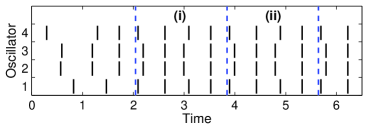
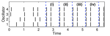
Figure 1: Firing times of four all-to-all pulse-coupled oscillators with $\tau=0.9$ and $\varepsilon=0.6$. Vertical dashed lines are used to indicate the boundaries of periods. (a) Initial phases $[\phi_{1}(0),\phi_{2}(0),\phi_{3}(0),\phi_{4}(0)]=[0.1766,0.4298,0.4079,0.7061]$. Two periods (i) and (ii) are presented. (b) Initial phases $[\phi_{1}(0),\phi_{2}(0),\phi_{3}(0),\phi_{4}(0)]=[0.4974,0.2492,0.8932,0.8501]$. Four periods (i), (ii), (iii) and (iv) are presented.

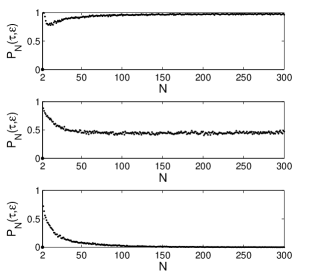
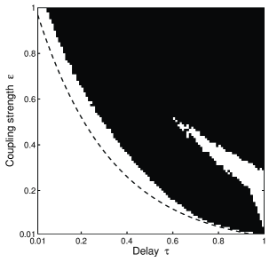
Figure 2: Dependence of $P_{N}(\tau,\varepsilon)$ on network size $N$. (a) $\tau=0.55$, $\varepsilon=0.4$. (b) $\tau=0.7$, $\varepsilon=0.35$. (c) $\tau=0.8$, $\varepsilon=0.3$.

Figure 3: Prevalence of completely synchronized solutions for $(\tau,\varepsilon)\in\mathcal{A}_{2}$. Parameters with $P_{100}(\tau,\varepsilon)>0$ are marked in black. The dashed curve represents $\{(\tau,\varepsilon)\in\mathcal{A}|f(\tau)+\varepsilon=1\}$.

Completely synchronized solutions, as a special type of periodic solutions, have been widely studied Mirollo1990 ; Mathar1996-Goel2002 ; Ernst1995 ; Ernst1998 ; Timme2002-2 ; Kim2004 ; Wu2007 . The following analysis demonstrates the different synchronization behaviors for networks with $(\tau,\varepsilon)\in\mathcal{A}_{1}$ and $(\tau,\varepsilon)\in\mathcal{A}_{2}$. In Wu2007 , we proved that under the assumption $f(2\tau)+\varepsilon<1$, from any initial phases (other than $\phi_{1}(0)=\cdots=\phi_{N}(0)$), all-to-all pulse-coupled oscillators with delayed excitatory coupling cannot achieve complete synchronization. In fact, we can extend this result to the case of $(\tau,\varepsilon)\in\mathcal{A}_{1}$ (see remark2 ). Interestingly, we found that when parameters $(\tau,\varepsilon)\in\mathcal{A}_{2}$, completely synchronized solutions become prevalent. In order to exhibit this, for networks with all-to-all coupling, we numerically estimate the fraction $P_{N}(\tau,\varepsilon)$ of the phase space $\mathbf{\Phi}:=\{(\phi_{1},\ldots,\phi_{N})|0<\phi_{i}\leq 1\}$ occupied by initial phases of completely synchronized solutions. We still use (5) for $f$. Fig. 3(a)-(c) show the dependence of $P_{N}(\tau,\varepsilon)$ on $N$ for $\tau=0.55$, $\varepsilon=0.4$; $\tau=0.7$, $\varepsilon=0.35$; and $\tau=0.8$, $\varepsilon=0.3$, respectively. More generally, we observed that $P_{N}(\tau,\varepsilon)$ converges to a constant depending on $(\tau,\varepsilon)$ as $N$ goes to infinity. For networks of $N=100$, Fig. 3 shows the region of parameter space $\mathcal{A}$ where completely synchronized solutions appear ($P_{100}(\tau,\varepsilon)>0$). For completely synchronized solutions, there must be some interspike intervals not exceeding the delay time $\tau$. Otherwise, the system cannot be completely synchronized (see Wu2007 ; remark2 ). The performance of Fig. 3 is supported by the observation Buck1988 of flashing patterns of two firefly species Photinus pyralis and Pteroptyx malaccae. For the species P. pyralis, the normalized delay (neural delay/endogenous flashing period) is $\approx 0.03$. The whole group of the species rarely synchronizes flashing; instead, wave, chain or sweeping synchrony has been reported. For the species P. malaccae, the normalized delay is $\approx 0.36$, and perfect synchrony is usually achieved.

In summary, our analysis demonstrates different dynamics for pulse-coupled networks with $(\tau,\varepsilon)\in\mathcal{A}_{1}$ and $(\tau,\varepsilon)\in\mathcal{A}_{1}$. For the region $\mathcal{A}_{1}$, we derive a low bound of interspike intervals and three firing properties, which provide a basis for future researches addressing the dynamics in networks, e.g., stability of periodic solutions. The difference of synchronization presented at the end of the Letter is useful for understanding and interpreting synchronization phenomena in some natural systems.

This work was supported by the National Science Foundation of China under Grants 60574044 and 60774074.

References

(1)
T. J. Walker, Science 166, 891 (1969); C. S. Peskin,
Mathematical Aspects of Heart Physiology (Courant Institute of
Mathematical Sciences, New York, 1975); L. F. Abbott and C. van
Vreeswijk, Phys. Rev. E 48, 1483 (1993); A. V. M. Herz and J.
J. Hopfield, Phys. Rev. Lett. 75, 1222 (1995); A. V. M. Herz
and J. J. Hopfield, Phys. Rev. Lett. 75, 1222 (1995).
(2)
J. Buck, Q. Rev. Biol. 63, 265 (1988).
(3)
R. E. Mirollo and S. H. Strogatz, SIAM J. Appl. Math. 50, 1645
(1990).
(4)
S. H. Strogatz and I. Stewart, Scientific American 269, 68
(1983).
(5)
C. van Vreeswijk and L. F. Abbott, SIAM J. Appl. Math. 53, 253
(1993); C. C. Chen, Phys. Rev. E 49, 2668 (1994); A. Corral
et al, Phys. Rev. Lett. 74, 118 (1995).
(6)
R. Mathar and J. Mattfeldt, SIAM J. Appl. Math. 56, 1094
(1996); P. Goel and B. Ermentrout, Physica D 163, 191 (2002).
(7)
U. Ernst, K. Pawelzik, and T. Geisel, Phys. Rev. Lett. 74,
1570 (1995).
(8)
U. Ernst, K. Pawelzik, and T. Geisel, Phys. Rev. E 57, 2150
(1998).
(9)
M. Timme, F. Wolf, and T. Geisel, Phys. Rev. Lett. 89, 154105
(2002).
(10)
M. Timme, F. Wolf, and T. Geisel, Phys. Rev. Lett. 89, 258701
(2002).
(11)
D. E. Kim, BioSystems 76, 7 (2004).
(12)
W. Wu and T. P. Chen, Nonlinearity 20, 789 (2007).
(13)
In Lemma 1 of Wu2007 , we prove that if the coupling is
all-to-all and parameters , satisfy
, then all interspike intervals of each
oscillator in the coupled system are longer than . For
normalized coupling and parameters
, the proof is simalar.
(14)
The proof is almost the same as that in Wu2007 . Here, we
briefly describe the proof process. By Theorem 1 in this Letter,
Lemma 1 in Wu2007 becomes that if an oscillator fires at time
and with , then . Although
the result of Lemma 1 is weakened, Lemmas 2-7 and Theorem 1 in
Wu2007 still hold. Moreover, all the derivations need not be
changed except that of Lemma 7. For the proof of Lemma 7, an
additional but straightforward case distinction is required.