Baryon Spectroscopy from Lattice QCD

Abstract

Progress in extracting excited-state baryon masses in lattice QCD using large sets of spatially-extended operators is presented. The use of stochastic estimates of all-to-all quark propagators with variance reduction techniques is described. Such techniques are crucial for incorporating multi-hadron operators into the correlation matrices of the hadron operators.

I INTRODUCTION

Experiments show that many excited-state hadrons exist, and there are significant experimental efforts to map out the QCD resonance spectrum, such as Hall B and the proposed Hall D at Jefferson Lab, ELSA associated with the University of Bonn, COMPASS at CERN, PANDA at GSI, and BESIII in Beijing. Hence, there is a great need for ab initio determinations of such states in lattice QCD.

To extract excited-state energies in Monte Carlo calculations, correlation matrices are needed and operators with very good overlaps onto the states of interest are crucial. To study a particular state of interest, all states lying below that state must first be extracted, and as the pion gets lighter in lattice QCD simulations, more and more multi-hadron states will lie below the excited resonances. To reliably extract these multi-hadron states, multi-hadron operators made from constituent hadron operators with well-defined relative momenta will most likely be needed, and the computation of temporal correlation functions involving such operators will require the use of all-to-all quark propagators. The evaluation of disconnected diagrams will ultimately be required. Perhaps most worrisome, most excited hadrons are unstable (resonances), so the results obtained for finite-box stationary-state energies in lattice QCD must be interpreted carefully.

In this talk, progress by the Hadron Spectrum Collaboration in extracting excited-state baryon masses in lattice QCD using large sets of spatially-extended operators is presented. The use of stochastic estimates of all-to-all quark propagators with variance reduction techniques is described. Such techniques are crucial for incorporating multi-hadron operators into correlation matrices.

II EXCITED STATIONARY STATES IN LATTICE QCD: KEY ISSUES

Capturing the masses of excited states requires the computation of correlation matrices $C_{ij}(t)=\langle 0|T\Phi_{i}(t)\Phi^{\dagger}_{j}(0)|0\rangle$ associated with a large set of $N$ different operators $\Phi_{i}(t)$. It has been shown in Ref. wolff90 that the $N$ principal effective masses $W_{\alpha}(t)$, defined by

$$W_{\alpha}(t)=\ln\left(\frac{\lambda_{\alpha}(t,t_{0})}{\lambda_{\alpha}(t+1,t_{0})}\right),$$

where $\lambda_{\alpha}(t,t_{0})$ are the eigenvalues of $C(t_{0})^{-1/2}\ C(t)\ C(t_{0})^{-1/2}$ and $t_{0}<t/2$ is usually chosen, tend to the eigenenergies of the lowest $N$ states with which the $N$ operators overlap as $t$ becomes large. When combined with appropriate analysis methods, such variational techniques are a particularly powerful tool for investigating excitation spectra.

The use of operators whose correlation functions $C(t)$ attain their asymptotic form as quickly as possible is crucial for reliably extracting excited hadron masses. An important ingredient in constructing such hadron operators is the use of smeared fields. Operators constructed from smeared fields have dramatically reduced mixings with the high frequency modes of the theory. Both link-smearing and quark-field smearing should be applied. Since excited hadrons are expected to be large objects, the use of spatially extended operators is another key ingredient in the operator design and implementation. Fig. 1 shows the different spatial configurations we use, which effectively build up the necessary orbital and radial structures of the hadron excitations. The basic building blocks in all of our hadron operators are covariantly-displaced quark or antiquark fields. These are first combined to have the appropriate flavor structure and color structure, then group-theoretical projections are applied to obtain operators which transform irreducibly under all lattice rotation and reflection symmetries. A more detailed discussion of these issues can be found in Ref. baryons1 .

Figure 1: The spatial arrangements of the extended three-quark baryon and quark-antiquark meson operators. Solid circles are smeared quark fields, open circles in the mesons are smeared “barred” antiquark fields, open circles in the baryons indicate a Levi-Civita color coupling, and solid line segments indicate covariant displacements.

A first glimpse of the higher-lying nucleon spectrum in lattice QCD was provided by the Hadron Spectrum Collaboration in Ref. adamthesis . These first results, shown in Fig. 2, were on small $12^{3}\times 48$ anisotropic quenched lattices with a very heavy pion. Results for both the nucleons and $\Delta$-resonances on 239 quenched configurations on a $16^{3}\times 64$ lattice and 167 quenched configurations on a $24^{3}\times 64$ lattice using an anisotropic Wilson action with spatial spacing $a_{s}\sim 0.1$ fm, $a_{s}/a_{t}\sim 3$, and a pion mass $m_{\pi}\sim 490$ MeV appeared during the past yearnucleons1 . These masses have also been determined in the past year using 430 $N_{f}=2$ configurations on a $24^{3}\times 64$ lattice with a stout-smeared clover fermion action and a Symanzik-improved anisotropic gauge actionnucleons2 . The results for a pion mass $m_{\pi}=400$ MeV, spacing $a_{s}\sim 0.1$ fm and $a_{s}/a_{t}\sim 3$ are shown in Fig. 2. The low-lying odd-parity band shows the exact number of states in each channel as expected from experiment. The two figures show the splittings in the band increasing as the quark mass is decreased. At these heavy pion masses, the first excited state in the $G_{1g}$ channel is significantly higher than the experimentally measured Roper resonance. It remains to be seen whether or not this level will drop down as the pion mass is further decreased. Most of the levels in the right-hand plot lie very close to two-particle thresholds. The use of two-hadron operators will be needed to go to lighter pion masses.

III MANY-TO-MANY QUARK PROPAGATORS

To study a particular eigenstate of interest, all eigenstates lying below that state must first be extracted, and as the pion gets lighter in lattice QCD simulations, more and more multi-hadron states will lie below the excited resonances. The correlation functions of such operators require estimates of the quark propagators from all spatial sites on a time slice to all spatial sites on another time slice. Computing all such elements of the propagators exactly is not possible (except on very small lattices). Some way of stochastically estimating them is needed.

Random noise vectors $\bm{\eta}$ whose expectations satisfy $E(\eta_{i})=0$ and $E(\eta_{i}\eta_{j}^{\ast})=\delta_{ij}$ are useful for stochastically estimating the inverse of a large matrix $M$ as follows. Assume that for each of $N_{R}$ noise vectors, we can solve the following linear system of equations: $MX^{(r)}=\eta^{(r)}$ for $X^{(r)}$. Then $X^{(r)}=M^{-1}\eta^{(r)}$, and

$$E(X_{i}\eta_{j}^{\ast})=E(\sum_{k}M^{-1}_{ik}\eta_{k}\eta_{j}^{\ast})=\sum_{k}M^{-1}_{ik}E(\eta_{k}\eta_{j}^{\ast})=\sum_{k}M^{-1}_{ik}\delta_{kj}=M^{-1}_{ij}.$$ (1)

The expectation value on the left-hand can be approximated using the Monte Carlo method. Hence, a Monte Carlo estimate of $M_{ij}^{-1}$ is given by

$$M_{ij}^{-1}\approx\lim_{N_{R}\rightarrow\infty}\frac{1}{N_{R}}\sum_{r=1}^{N_{R}}X_{i}^{(r)}\eta_{j}^{(r)\ast},\qquad\mbox{where $MX^{(r)}=\eta^{(r)}$.}$$ (2)

This equation usually produces stochastic estimates with variances which are much too large to be useful.

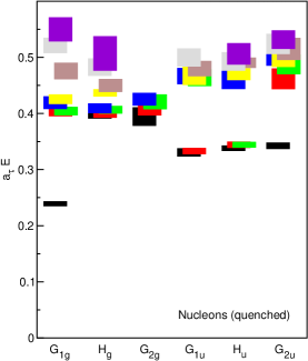
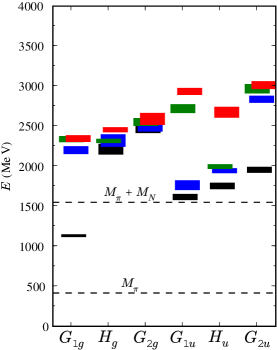
Figure 2: (Left) Nucleon spectrum from 200 quenched configurations on a $12^{3}\times 48$ anisotropic lattice using the Wilson gauge and quark actions with $a_{s}\sim 0.1$ fm, $a_{s}/a_{t}\sim 3.0$ and $m_{\pi}\sim 700$ MeV from Ref. adamthesis . (Right) Nucleon spectrum from 430 $N_{f}=2$ configurations on a $24^{3}\times 64$ lattice using a stout-smeared clover fermion action and Symanzik-improved gauge action with $a_{s}\sim 0.1$ fm, $a_{s}/a_{t}\sim 3$, and $m_{\pi}=400$ MeV from Ref. nucleons2 .

Progress is only possible if stochastic estimates of the quark propagators with reduced variances can be made. A technique of diluting the noise vectors has been developed which accomplishes such a variance reductiondilute1 . A given dilution scheme can be viewed as the application of a complete set of projection operators. To see how dilution works, consider a general $N\times N$ matrix $M$ having matrix elements $M_{ij}$. Define some complete set of $N\times N$ projection matrices $P^{(a)}$ which satisfy $P^{(a)}P^{(b)}=\delta^{ab}P^{(a)}$ with $\sum_{a}P^{(a)}=1$ and $P^{(a)\dagger}=P^{(a)}$. Then observe that

$$M_{ij}^{-1} = M_{ik}^{-1}\delta_{kj}=\sum_{a}M_{ik}^{-1}P^{(a)}_{kj}=\sum_{a}M_{ik}^{-1}P^{(a)}_{kk^{\prime}}P^{(a)}_{k^{\prime}j}=\sum_{a}M_{ik}^{-1}P^{(a)}_{kk^{\prime}}\delta_{k^{\prime}j^{\prime}}P^{(a)}_{j^{\prime}j}$$ (3)

$$= \sum_{a}M_{ik}^{-1}P^{(a)}_{kk^{\prime}}E(\eta_{k^{\prime}}\eta^{\ast}_{j^{\prime}})P^{(a)}_{j^{\prime}j}=\sum_{a}M_{ik}^{-1}E\left(P^{(a)}_{kk^{\prime}}\eta_{k^{\prime}}\eta^{\ast}_{j^{\prime}}P^{(a)}_{j^{\prime}j}\right).$$

Define $\eta^{[a]}_{k}=P^{(a)}_{kk^{\prime}}\eta_{k^{\prime}}$ and $\eta^{[a]\ast}_{j}=\eta^{\ast}_{j^{\prime}}P^{(a)}_{j^{\prime}j}=P^{(a)\ast}_{jj^{\prime}}\eta^{\ast}_{j^{\prime}},$ and further define $X^{[a]}$ as the solution of $M_{ik}X^{[a]}_{k}=\eta^{[a]}_{i},$ then we have

$$M_{ij}^{-1}=\sum_{a}M_{ik}^{-1}E(\eta^{[a]}_{k}\eta^{[a]\ast}_{j})=\sum_{a}E(X^{[a]}_{i}\eta^{[a]\ast}_{j}).$$ (4)

Although the expected value of $\sum_{a}\eta^{[a]}_{k}\eta^{[a]\ast}_{j}$ is the same as $\eta_{k}\eta^{\ast}_{j}$, the variance of $\sum_{a}\eta^{[a]}_{k}\eta^{[a]\ast}_{j}$ is significantly smaller than that of $\eta_{k}\eta^{\ast}_{j}$. For both $Z_{4}$ and $U(1)$ noise, we have $Var({\rm Re}(\eta_{i}\eta_{j}^{\ast}))=Var({\rm Im}(\eta_{i}\eta_{j}^{\ast}))=\textstyle\frac{1}{2}(1-\delta_{ij}).$ Although the variance is zero for $i=j$, there is a significant variance for all $i\neq j$. The dilution projections ensure exact zeros for many of the off-diagonal elements, instead of values that are only statistically zero. In other words, many of the $i\neq j$ elements become exactly zero.

Of course, the effectiveness of the variance reduction depends on the projectors chosen. A particularly important dilution scheme for measuring temporal correlations in hadronic quantities is “time dilution” where the noise vector is broken up into pieces which only have support on a single time slice. Spin and color dilution are two other easy-to-implement schemes, and various spatial dilution schemes are possible. These various dilution projectors can also be combined to make hybrid schemes.

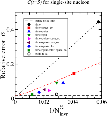
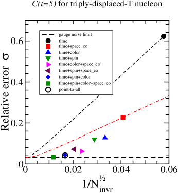
Figure 3: (Left) The relative errors in the correlation function of a single-site nucleon operator for temporal separation $t=5a_{t}$ evaluated using stochastically-estimated quark propagators with different dilution schemes against $1/N_{\rm inv}^{1/2}$, where $N_{\rm inv}$ is the number of Dirac matrix inversions required. The open circle shows the point-to-all error, and the horizontal dashed line shows the gauge-noise limit. The black (red) dashed-dotted line shows the decrease in error expected by simply increasing the number of noise vectors, starting from the time (time + even/odd-space) dilution point. (Right) Same as the left plot, except for a triply-displaced-T nucleon operator. These results used 100 quenched configurations on a $12^{3}\times 48$ lattice.

A comparison of the different dilution schemes is shown in Fig. 3. These computations are dominated by the inversions of the Dirac matrix, so using the number of matrix inversions $N_{\rm inv}$ to compare computational efforts is reasonably fair. The advantage in using increased dilutions compared to an increased number of noise vectors with only time dilution is evident in the plots. However, this advantage quickly diminishes after time + even/odd-space dilution, or time+color, or time+spin dilution. These encouraging results demonstrate that the inclusion of good multi-hadron operators will certainly be possible using stochastic all-to-all quark propagators with diluted-source variance reduction.

IV SUMMARY AND OUTLOOK

This talk discussed the key issues and challenges in exploring excited hadrons in lattice QCD. The importance of multi-hadron operators and the need for all-to-all quark propagators were emphasized. The technology needed to extract excited stationary-state energies, including operator design and field smearing, was detailed. Efforts in variance reduction of stochastically-estimated all-to-all quark propagators using source dilutions was described.

Given the major experimental efforts to map out the QCD resonance spectrum, such as Hall B and the proposed Hall D at Jefferson Lab, ELSA, COMPASS, PANDA, and BESIII, there is a great need for ab initio determinations of such states in lattice QCD. The exploration of excited hadrons in lattice QCD is well underway.

- (1) M. Lüscher and U. Wolff, Nucl. Phys. B339, 222 (1990).
- (2) S. Basak, R.G. Edwards, G.T. Fleming, U.M. Heller, C. Morningstar, D. Richards, I. Sato, S. Wallace, Phys. Rev. D72, 094506 (2005).
- (3) A. Lichtl, Ph.D. thesis, Carnegie Mellon University [hep-lat/0609019].
- (4) S. Basak, R. Edwards, G. Fleming, K. Juge, A. Lichtl, C. Morningstar, D. Richards, I. Sato, S. Wallace, Phys. Rev. D76, 074504 (2007).
- (5) J. Bulava, J. Foley, C. Morningstar, J. Dudek, R. Edwards, B. Joo, H.W. Lin, D. Richards, E. Engelson, S. Wallace, A. Lichtl, N. Mathur, in preparation (also, see these proceedings).
- (6) J. Foley, K.J. Juge, A. O’Cais, M. Peardon, S. Ryan, J.I. Skullerud, Comput. Phys. Commun. 172, 145 (2005).