The staircase structure of the Southern Brazilian Continental Shelf

Abstract

We show some evidences that the Southeastern Brazilian Continental Shelf (SBCS) has a devil’s staircase structure, with a sequence of scarps and terraces with widths that obey fractal formation rules. Since the formation of these features are linked with the sea level variations, we say that the sea level changes in an organized pulsating way. Although the proposed approach was applied in a particular region of the Earth, it is suitable to be applied in an integrated way to other Shelves around the world, since the analyzes favor the revelation of the global sea level variations.

I Introduction

During the late quaternary period, after the last glacial maximum (LGM), from 18 kyears ago till present, a global warming was responsible for the melting of the glaciers leading to a fast increase in the sea level. In approximately 13 kyears, the sea level rised up to about 120 meters, reaching the actual level. However, the sea level did not go up in a continuous fashion, but rather, it has evolved in a pulsatile way, leaving behind a signature of what actually happened, the Continental Shelf, i.e. the seafloor.

Continental shelves are located at the boundary with the land so that they are shaped by both marine and terrestrial processes. Sea-level oscillations incessantly transform terrestrial areas in marine environments and vice-versa, thus increasing the landscape complexity lambeck:2001 . The presence of regions with abnormal slope as well as the presence of terraces on a Continental Shelf are indicators of sea level positions after the Last Glacial Maximum (LGM), when large ice sheets covered high latitudes of Europe and North America, and sea levels stood about 120-130m lower than today heinrich:1988 . Geomorphic processes responsible for the formation of these terraces and discontinuities on the bottom of the sea topography are linked to the coastal dynamics during eustatic processes associated with both erosional or depositional forcing (wave cut and wave built terraces respectively goslar:2000 ).

The irregular distribution of such terraces and shoreface sediments is mainly controlled by the relationship between shelf paleo-physiography and changes on the sea level and sediment supply which reflect both global and local processes. Several works have dealt with mapping and modeling the distribution of shelf terraces in order to understand the environmental consequences of climate change and sea level variations after the LGM adams:1999 ; andrews:1998 ; broecker:1998 .

In this period of time the sea-level transgression was punctuated by at least six relatively short flooding events that collectively accounted for more than 90m of the 120m rise. Most (but not all) of the floodings appear to correspond with paleoclimatic events recorded in Greenland and Antarctic ice-cores, indicative of the close coupling between rapid climate change, glacial melt, and corresponding sea-level rise taylor:1997 .

In this work, we analyze data from the Southeastern Brazilian Continental Shelf (SBCS) located in a typical sandy passive margin with the predominance of palimpsests sediments. The mean length is approximately 250km and the shelfbreak is located at 150m depth. It is a portion of a greater geomorphologic region of the southeastern Brazilian coast called São Paulo Bight, an arc-shaped part of the southeastern Brazilian margin. The geology and topography of the immersed area are very peculiar, represented by the Mesozoic/Cenozoic tectonic processes that generated the mountainous landscapes known as ”Serra do Mar”. These landscapes (with mean altitudes of 800m) have a complex pattern that characterize the coastal morphology, and leads to several scarps intercalated with small coastal plains and pocket beaches.

This particular characteristic determines the development of several small size fluvial basins and absence of major rivers conditioning low sediment input, what tends to preserve topographic signatures of the sea-level variations.

For the purpose of the present study, we select three parallel profiles acquired from echo-sounding surveys, since for all the considered profiles, the same similar series of sequences of terraces were found. These profiles furtado:1992 ; conti:2001 ; correa:1996 are transversal to the coastline and the isobaths trend, and they extend from a 20m to a 120m depth.

The importance of understanding the formation of these ridges is that it can tell us about the coastal morphodynamic conditions, inner shelf processes and about the characteristics of periods of the sea level regimes standstills (paleoshores). In particular, the widths of the terraces are related to the time the sea level ”stabilized”. All this information is vital for the better understanding of the late quaternary climate changes dynamic.

We find relations between the widths of the terraces that follow a self-affine pattern description. These relations are given by a mathematical model, which describes an order of appearance for the terraces. Our results suggest that this geomorphological structure for the terraces can be described by a devil’s staircase mandelbrot:1977 , a staircase with infinitely many steps in between two steps. This property gives the name ”devil” to the staircase, once an idealized being would take an infinite time to go from one step to another. So, the seafloor morphology is self-affine (fractal structure) as reported in Ref. herzfeld ; goff , but according to our findings, it has a special kind of self-affine structure, the devil’s staircase structure.

A devil’s staircase as well as other self-affine structure are the response of an oscillatory system when excited by some external force. The presence of a step means that while varying some internal parameter, the system preserves some averaged regular behavior, a consequence of the stable frequency-locking regime between a natural frequency of the system and the frequency of the excitation. This staircase as well as other self-affine structures are characterized by the presence of steps whose widths are directly related to the rational ratio between the natural frequency of the system and the frequency of the excitation.

In a similar fashion, we associate the widths of the terraces with rational numbers that represent two hypothetical frequencies of oscillation which are assumed to exist in the system that creates the structure of the SBCS, here regarded as the sea level dynamics (SLD), also known as the sea level variations. Then, once these rational numbers are found, we show that the relative distances between triples of terraces (associated with some hypothetical frequencies) follow similar scalings found in the relative distance between triples of plateaus (associated with these same frequencies) observed in the devil’s staircase.

The seafloor true structure, apart from the dynamics that originated it, is also a very relevant issue, specially for practical applications. For example, one can measure the seafloor with one resolution and then reconstruct the rest based on some modeling mareschal . As we show in this work (Sec. V), a devil’s staircase structure fits remarkably well the experimental data.

Our paper is organized as follows. In Sec. II, we describe the data to be analyzed. In Sec. III, we describe which kind of dynamical systems can create a devil’s staircase and how one can detect its presence in experimental data based on only a few observations. In Sec. IV, we show the evidences that led us to characterize the SBCS as a devil’s staircase, and in Sec. V we show how to construct seafloor profiles based on the devil’s staircase geometry. Finally, in Sec. VI, we present our conclusions, discussing also possible scenarios for the future of the sea level dynamics under the perspective of our findings.

II Data

Figure 1: [Color online] Profiles (depth versus the distance to the cost) of the Southeastern Brazilian Continental Shelf. The arrows indicate the terraces considered in our analyzes. The profile shown with a thick black line is the profile chosen for our derivations, reproduced also in (B). The other two profiles had their original position of the two axes shifted by a constant value such that one can also identify the terraces observed in the chosen profile in these other two. Note that a translation of the profiles by a constant value has no effect on any of the scalings observed. The reason of this mismatch between the profiles is due to the local geometry of the cost at the time the sea reached that level.

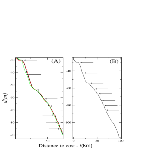
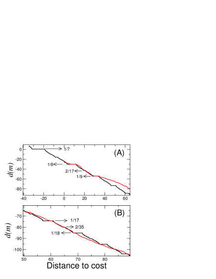
The data consists of the tree profiles given in Fig. 1(A-B). The profile considered for our analyzes is shown in Fig. 1(B), where we show the Continental Shelf of the State of São Paulo, in a transversal cut in the direction: inner shelf (”cost”) $\rightarrow$ shelfbreak (”open sea”). The horizontal axis represents the distance to the cost and the vertical axis, the sea level (depth), $d$. We are interested in the terraces widths and their respective depths.

The profiles shown in Fig. 1 were the result of a smoothing (filtering) process from the original data collected by Sonar note3 . The smoothing process is needed to eliminate from the measured data the influence of the oscillations of the ship where the sonar is located and local oscillations on the sea floor probably due to the stream flows.

Smaller topographic terraces could be smoothed or masked due to several processes such as: coastal dynamic erosional during sea-level rising, Holocene sediment cover, erosional processes associated with modern hidrodynamic pattern (geostrophic currents). For that reason we only consider the largest ones, as the ones shown in Fig. 2, (located at $d=-30.01m$ with the width of $l=6.06km$). As one can see, the edges of the terraces are not so sharp as one would expect from a staircase plateau. Again, this is due to the action of the sea waves and stream flows throughout the time. To reconstruct what we believe to be the original terrace, we consider that its depth is given by the depth of the middle point, and its width is given by the minimal distance between two parallel lines placed along the scarps of the terrace edges. Using this procedure, we construct Table 1 with the largest and more relevant terraces found.

We identify a certain terrace introducing a lower index $n$ in $l$ and $d$, according to their chronological order of appearance. More recent appearance (closer to the cost, less deep) smaller is the index $n$. We consider the more recent data to have a zero distance from the cost, but in fact, this data is positioned at about 15km away from the shore, where the bottom of the sea is not affected by the turbulent zone caused by the break out of the waves. The profile of Fig. 1(B) was the one chosen among the other tree profiles because from it we could more clearly identify the largest number of relevant terraces note3 .

Figure 2: Reconstruction of the terraces. The width of the terrace is given by the minimal distance between the two parallel dashed lines.

$n$	$d_{n}(m)$	$l_{n}(km)$
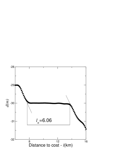
1	-30.01	6.06 $\pm$ 0.05
2	-41.86	1.59 $\pm$ 0.05
3	-54.01	2.93 $\pm$ 0.05
4	-61.14	1.73 $\pm$ 0.05
5	-66.69	2.21 $\pm$ 0.05
6	-74.33	0.80 $\pm$ 0.1
7	-79.75	0.80 $\pm$ 0.1
8	-85.30	0.80 $\pm$ 0.1

Table 1: Terrace widths and depths. While the depths present no representative deviation, the deviation in the widths become larger for deeper terraces. The deviation in the widths is estimated by calculating the widths assuming many possible configurations between the placement of the two parallel lines used to calculate the widths.

III The Devil’s Staircase

Frequency-locking is a resonant response occurring in systems of coupled oscillators or oscillators coupled to external forces. The first relevant report about this phenomenon was given by Christian Huygens in the 17${}^{t}h$ century. He observed that two clocks back to back in the wall, set initially with slightly different frequencies, would have their oscillations coupled by the energy transfer throughout the wall, and then they would eventually have their frequencies synchronized. Usually, we expect that an harmonic, $P_{w1}$, of one oscillatory system locks with an harmonic, $Q_{w2}$, of the other oscillatory system, leading to a locked system working in the rational ratio $P/Q$ jensen:1984 .

To understand what is the dynamics responsible for the onset of a frequency-locked oscillation, that is, the reasons for which a system either locks or unlocks, we present the simplest model one can come up with to describe a more general oscillator. This model is described by an angle $\theta$, which is changed (after one period) to the angle $f(\theta)$. So, $f(\theta)=\theta+\Omega$. In order to introduce an external force in the oscillator modeling also possible physical interactions with other oscillators, a resonant term, $g$, is added into this model, resulting in the following model

$$f(\theta)=\theta+\Omega-g(\theta,K)\mbox{\ \ \ }(mod\mbox{\ }1),$$ (1)

where

$$g(\theta,K)=\frac{K}{2\pi}\sin{2\pi\theta}.$$ (2)

Despite this map simplicity, the same can not be said about its complexity argyris:1994 . Arnold (see ref. arnold:1965 ) studied this map in detail aiming to understand how an oscillatory system would undergo into periodic stable state when perturbed by an external perturbation.

For $K=0$, Eq. (1) represents a pure rotation, which is topological equivalent to a twice continuously differentiable, orienting preserving mapping of the circle onto itself [Theorem of Denjoy, see Ref. arnold:1988 ]. Therefore, the simple Eq. (1) can be considered as a model for many types of oscillatory systems. In fact, Eq. (1) represents a more complicated system, a three-dimensional torus with frequencies $w_{1}$ and $w_{2}$, when viewed by a Poincaré map. Thus, $\Omega$ in Eq. (1) represents the ratio $w_{1}/w_{2}$. When $w_{1}/w_{2}=p/q$ (with $p\leq q$) is rational, this map has a period $p$ motion and its trajectory, i.e. the value of $\theta$, assumes the same value after $q$ iterations. For $K=0$, the so called winding number $W$ is exactly equal to $\Omega$, i.e. $W$=$p/q$.

For $K\neq 0$ (non-linear case) $W$ is defined by

$$W(\Omega,K)=\lim_{n\to\infty}\frac{h(\theta_{0},K)+h(\theta_{1},K)+\ldots+h(\theta_{n-1},K)}{n},$$ (3)

where

$$h(\theta,K)=\Omega+g(\theta,K).$$ (4)

For $K<1$, Eq. (1) is monotonic and invertible. For $K=1$, it develops a cubic inflection point at $\theta=0$. The map is still invertible but the inverse has a singularity. For $K>1$ the map is non-invertible.

Figure 3: A complete devil’s staircase, obtained from Eq. (1), for $K$=1.

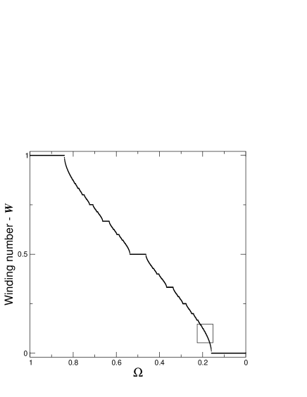
Arnold wanted to understand how periodic oscillations would appear as one increases $K$ from zero to positive values. He observed that a quasi-periodic oscillation, for an irrational $\Omega$ and $K=0$, would turn into a periodic oscillation as one varies $K$, from zero to positive values. He demonstrated that a periodic oscillation has probability zero of being found for $K=0$ (rational numbers set is countable while the irrational numbers set is uncountable) and positive probability of being found for $K>0$. He also observed that fixing a positive value $K$, the winding number $W$ [Eq. (3)] is a continuous but not differentiable function of $\Omega$, as one can see in Fig. 3, forming a stair-like structure.

If $W(\Omega,K)$ is rational, it can be represented by the ratio between two integer numbers as $W=\frac{P}{Q}$. At this point, the frequency $\Omega$ and the frequency of the function $g$ are locked, producing the phenomenon of frequency-locking, when $W(K,\Omega)$ does not change its value within an interval $\Delta\Omega$ (a plateau) of values of $\Omega$. In fact, smaller is the denominator $Q$, larger is the interval $\Delta\Omega$.

As one changes $\Omega$, plateaus for $W$ rational appear following a natural order described by the Farey mediant. Given two plateaus that represent a $\frac{P_{1}}{Q_{1}}$ and a $\frac{P_{3}}{Q_{3}}$ winding numbers, with plateau widths of $\Delta\Omega_{1}$ and $\Delta\Omega_{3}$, respectively, there exists another plateau positioned at a winding number $W$ within the interval $[\frac{P_{1}}{Q_{1}},\frac{P_{3}}{Q_{3}}]$ given by

$$\frac{P_{2}}{Q_{2}}=\frac{P_{1}+P_{3}}{Q_{1}+Q_{3}}.$$ (5)

The Farey mediant gives the rational with the smallest integer denominator that is within the interval $[\frac{P_{1}}{Q_{1}},\frac{P_{3}}{Q_{3}}]$. Therefore, the $\Delta\Omega(\frac{P_{2}}{Q_{2}})$ plateau is smaller than $\Delta\Omega(\frac{P_{1}}{Q_{1}})$ and $\Delta\Omega(\frac{P_{3}}{Q_{3}})$, but is bigger than any other possible plateau. Organizing the rationals according to the Farey mediant creates an hierarchical level of rationals, which are called Farey Tree. The plateaus $\Delta\Omega_{1}$ and $\Delta\Omega_{3}$ are regarded as the parents, and $\Delta\Omega_{2}$ as the daughter plateau.

The interesting case of Eq. (1) for our purpose, is exactly when $K$=1. For that case, one can find periodic orbits with any possible rational winding number, as one varies $\Omega$. What results in a zero (probability) measure of finding quasi-periodic oscillation in Eq. (1), by a random chosen of the $\Omega$ value. Also, for $K>1$, due to the overlap of resonances (periodic oscillation), chaos is possible.

The devil’s staircase can be fully characterized by the relations between the plateaus widths, and the relations between the gaps between two of them. While the plateau widths are linked to the probability one has to find periodic oscillations, the gaps widths between plateaus are linked to the probability one has to find quasi-periodic oscillations, in Eq. (1).

There are many scaling laws relating the plateau widths jensen:1983 ; jensen:1984 ; cvitanovic:1985 . There are local scalings, which relate the widths of plateaus that appear close to a specific winding number, for example the famous golden mean $W_{G}=\frac{\sqrt{5}-1}{2}$. However, we will focus our attention in the global scalings, which can be experimentally observed, and only for the case where $K$=1. For this case, we are interested in two scalings. The one that relates the plateau widths with the respective winding numbers in the form $\frac{1}{Q}$ (the largest plateaus), and the one that describes the structure of the complementary set to the plateaus $\Delta\Omega$, i.e. the structure of the gaps between plateaus. The structure of the plateaus is a Cantor set as well as the structure of the complementary set. Therefore, a characterization of these sets can be done in terms of the fractal dimension $D_{0}$ farmer:1983 of the complementary set.

The first scaling is jensen:1984

$$\Delta\Omega(\frac{1}{Q})\propto\frac{1}{Q^{\gamma}}\mbox{\ \ }(\gamma>3),$$ (6)

The second scaling relates the widths of the complementary set as one goes to smaller and smaller scales. These widths are related to a power-scaling law whose coefficient $D_{0}$ is the fractal dimension of the complementary set. For $K=1$, we have that the fractal dimension of the complementary set is $D_{0}\cong 0.87$. This is an universal scaling. Since the complementary set of the plateaus represents the irrational rotations, the smaller is its fractal dimension, the smaller is the probability of finding quasi-periodic oscillation.

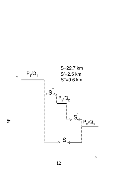
For experimental data, the determination of $D_{0}$ is difficult to obtain because the dimension measures a microscopic quantity of the plateaus widths, and in experimental data one can only observe the largest plateaus. Fortunately, an approximation $D^{\prime}$ for $D_{0}$ can be obtained from the largest plateaus by using the idea proposed in hentschel:1983 ,

$$\left(\frac{S^{\prime}}{S}\right)^{D^{\prime}}+\left(\frac{S^{\prime\prime}}{S}\right)^{D^{\prime}}=1.$$ (7)

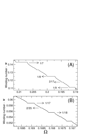
where $S^{\prime}$, $S$, and $S^{\prime\prime}$ are represented in Fig. 4.

Figure 4: Representation of the gaps $S^{\prime\prime}$, $S^{\prime}$, and $S$, used to estimate the fractal dimension $D_{0}$ of the complementary set, using Eq. (7).

In case one has $K\cong 1$ ($K<1$), we do not have a complete devil’s staircase. In other words, winding numbers with denominators larger than a given ${\widetilde{Q}}$ are cut off from the Farey Tree. Using this information we can estimate the value of $K$ through the largest denominator observed jensen:1984

$${\widetilde{Q}}\geq\frac{1}{1-K}.$$ (8)

Finally, we would like to stress that while in Eq. (1) the plateaus of the devil’s staircase are positioned at winding numbers defined by Eq. (3), in nature, devil’s staircases have plateaus positioned at some accessible measurement.

In the driven Rayleigh-Bénard experiment stavans:1985 ; jensen:1985 , convection rolls appear in a small brick-shaped cell filled with mercury, for a critical temperature difference between the upper and lower plates. As one perturbs the cell by a constant external magnetic field parallel to the axes of the rolls and by the introduction of an AC electrical current sheet pulsating with a frequency $f_{e}$ and amplitude $B$, a devil’s staircase is found in the variable $f_{i}$, the main frequency of the power spectra of the fluid velocity. As one varies the external frequency $f_{e}$, stable oscillations take place at a frequency ratio $f_{i}/f_{e}$, for a given value of $f_{e}$. In analogy to the devil’s staircase of Eq. (1), $f_{e}$ should be thought as playing the same role of $\Omega$ in Eq. (1), and the ratio $f_{i}/f_{e}$ as playing the same role of the winding number $W$.

A devil’s staircase can also be observed (see Ref. baptista:2004 ) in the amount of information $H$ (topological entropy) that an unstable chaotic set has in terms of an interval of size $\epsilon$, used to create the set. To generate the unstable chaotic set, we eliminate all possible trajectories of a stable chaotic set that visits this interval $\epsilon$. In analogy with the devil’s staircase of the circle map, $\epsilon$ should be related to $\Delta\Omega$, while $H$ to $W$.

The first proof of a complete devil’s staircase in a physical model was given in Ref. bak:1982 , in the one-dimensional ising model with convex long-range antiferromagnetic interactions.

In Ref. jin:1994 , it was found that a model for the El Niño, a phenomenon that is the result of a tropical ocean-atmosphere interaction when coupled nonlinearly with the Earth’s annual cycle, could undergo a transition to chaos through a series of frequency-locked steps. The overlapping of these resonances, which are the steps of the devil’s staircase, leads to the chaotic behavior.

IV A devil’s staircase in the Southern Brazilian Continental Shelf

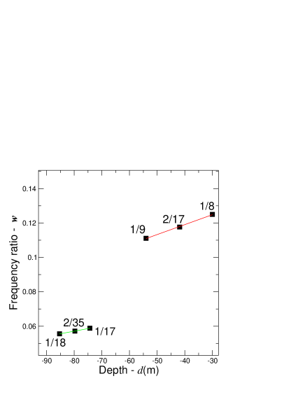
The main premise that guides the application of the devil’s staircase model to the Shelf is that the rules found in quantities related to the widths and depths of the terraces obey the same rules found in a complete devil’s staircase for the frequency-locked intervals $\Delta\Omega$ and their rational winding number, $W$. Thus, we assume that the terrace widths $l_{n}$ play the same role of the frequency-locked intervals $\Delta\Omega$, and the terrace depths play the same role of the rational winding number $W$.

In order to interpret the Shelf as a devil’s staircase, we have to show that the terraces appear in positions which respect the Farey mediant, the rule that describes the winding number ”positions” of the many plateaus. For that, we verify whether the position of the terraces at $d_{n}$ can be associated to hypothetical frequency ratios, denoted by $w_{n}=\frac{p_{n}}{q_{n}}$, which respects the Farey mediant. In doing so, we want that the metric of three adjacent terraces respects the Farey mediant. In addition, we also assume that the larger terraces are the parents of the Farey Tree, while the smaller terraces between two larger ones are the daughters. Thus, for each triple of terrace, we want that

$$\frac{d_{n+2}+d_{n}}{d_{n+1}}=\frac{w_{n+2}+w_{n}}{w_{n+1}}.$$ (9)

One could have considered other ways to relate the depths and the frequency ratios. The one chosen in Eq. (9) is used in order to account for the fact that while $d_{n}$ is negative $w_{n}$ is not.

From Eq. (9) it becomes clear that for the further analysis the depth of a particular terrace does not play a so important role as the ratio between the depths of triple of terraces that contains this particular terrace. These ratios may eliminate the influence of the local morphology and the influence of the local sea level dynamics into the formation of the Shelf. Therefore, the proposed quantity might be suitable for an integrate analysis of the different Shelfs all over the world, specially the ones affected by local geomorphological characteristics.

From the Farey mediant, we have a way to obtain the frequency ratios associated to each terrace,

$$w_{n+1}=\frac{p_{n}+p_{n+2}}{q_{n}+q_{n+2}}.$$ (10)

Therefore, combining Eq. (9) and Eq. (10), we obtain

$$\frac{p_{n}+p_{n+2}}{q_{n}+q_{n+2}}=\frac{\frac{p_{n+2}}{q_{n+2}}+\frac{p_{n}}{q_{n}}}{E},$$ (11)

which results in

$$(p_{n}+p_{n+2})(E-1)q_{n}q_{n+2}p_{n}=p_{n}q_{n+2}^{2}+q_{n}^{2}p_{n+2},$$ (12)

where $E$ is defined by

$$\frac{d_{n+2}+d_{n}}{d_{n+1}}=E.$$ (13)

$n$	$p_{n}$	$q_{n}$
1	1	8
2	2	17
3	1	9
4	-	-
5	-	-
6	1	17
7	2	35
8	1	18

Table 2: Integers associated with the $n$ considered terraces, with $n=1,\ldots,8$.

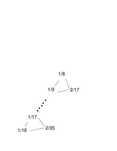
We do not expect to have Eq. (12) satisfied. We only require that the difference between the left and right hand sides of this equation, regarded as $\delta\epsilon$, is the lowest possible, among all possible values for $p_{m}$ and $q_{m}$ (with $m=n,n+2$), for a given $E$, with the restriction that the considered largest terraces are related to largest plateaus of Eq. (1), and thus $p_{m+2}$=$p_{m}$ and $q_{m+2}$=$q_{m}+1$, and $\delta\epsilon\ll 1$. Doing so, we find the rationals associated with the terraces, which are shown in table 2. The minimal value of $\delta\epsilon$, denoted by $\min{[\delta\epsilon]}$, is $\min{[\delta\epsilon(d_{1},d_{2},d_{3})]}$=0.032002, with $p_{1}/q_{1}$=$1/8$ for the terrace 1, and $p_{3}/q_{3}$=$1/9$, for the terrace 3. We also find that $\min{[\delta\epsilon(d_{6},d_{7},d_{8})]}$=0.002344, with $p_{6}/q_{6}$=$1/17$, for the terrace 6, and $p_{8}/q_{8}$=$1/18$, for the terrace 8. These minimal values can be seen in Figs. 5(A-B), where we show the values of $\delta\epsilon(d_{1},d_{2},d_{3})$ [in (A)] and the values of $\delta\epsilon(d_{6},d_{7},d_{8})$ [in (B)], for different values of $p$ and $q$. Using bigger values for $p$ has the only effect to increase the value of $\delta\epsilon$.

We have not identified rationals that can be associated with the terraces $4$ and $5$, which means that for $p$ and $q$ within $p=[1,50]$ and $q=[1,400]$, we find that $\delta\epsilon>1$. We have assumed that they could be either a daughter or a parent.

From now on, when convenient, we will drop the index $n$ and represent each terrace by the associated frequency ratio. So, the terrace 1, for $n$=1, is represented as the terrace with $w=1/8$.

Figure 5: [Color online] (A) Values of $\delta\epsilon(d_{1},d_{2},d_{3})$ and (B) $\delta\epsilon(d_{6},d_{7},d_{8})$, for different values of $p$ and $q$. $\delta\epsilon$ is the difference between the left and the right hand sides of Eq. (12).

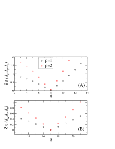
Table 2 can be represented in the form of the Farey Tree as shown in Fig. 6. The branch of rationals in the Farey Tree in the form $1/q$ belongs to the most stable branch, which means that the observed terraces should have the largest widths. We believe that the other less important branches of the complete devil’s staircase present in the data were smoothed out by the action of the waves and the flow streams throughout the time, and at the present time cannot be observed.

Notice that as the time goes by, the frequency ratios are increasing their absolute value, which means that if this tendency is preserved in the future, we should expect to see larger terraces.

Figure 6: Farey Tree representing the frequency ratios associated with the major terraces.

Figure 7: Scaling between the $1/q$-terrace widths and the value of $q$.

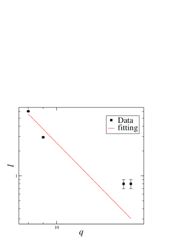
In the following, we will try to recover in the experimental profile, the universal scaling laws of Eqs. (6) and (7). Regarding Eq. (6), we find that $l$ scales as $1/q^{-3.60}$, as shown in Fig. 7, which is the expected global universal scaling for a complete devil’s staircase. Regarding Eq. (7), and calculating $S^{\prime}$, $S^{\prime\prime}$, and $S$ using the triple of terraces with widths $l(w=1/8)$, $l(w=2/17)$, and $l(w=1/9)$, as represented in Fig. 4, we find $D^{\prime}$=0.89. Using the triple of terraces ($n$=3,$n$=4,$n$=5), we find that $D^{\prime}$=0.87. Both results are very close from the universal fractal dimension $D_{0}\cong 0.87$, found for a complete devil’s staircase.

V Fitting the SBCS

Figure 8: Magnifications of the small box of Fig. 3, showing the plateaus of the devil’s staircase of Eq. (1) that appear for the same frequency ratios associated with the triple of terraces $w$=(1/8,2/17,1/9), in (A), and $w$=(1/17,2/35,1/18), in (B).

Motivated by our previous results, we fit the observed Shelf as a complete devil’s staircase, using Eq. (1). Notice that the only requirement for Eq. (1) to generate a complete devil’s staircase is that the function $g$ has a cubic inflection point at the critical parameter $K=1$. Whether Eq. (1) is indeed an optimal modeling for the Shelf is beyond the scope of the present study. We only chose this map because it is a well known system and it captures most of the relevant characteristic a dynamical systems needs to fulfill in order to create a devil’s staircase.

We model the SBCS as a complete devil’s staircase, but we rescale the winding number $W$ into the observed terrace depth. So, we transform the complete devil’s staircase of Fig. 8 as good as possible into the profile of Fig. 1(B), by rescaling the vertical axis of the staircase in Fig. 8.

We do that by first obtaining the function $F$ (see Fig. 9) whose application into the terrace depth $d(w)$ gives the frequency ratio $w_{n}=\frac{p_{n}}{q_{n}}$ associated with the terrace.

For the triple of terraces $w$=(1/8,2/17,1/9), we obtain

$$F(d[km])=0.14219+0.00057853d[km],$$ (14)

and for the triple of terraces $w$=(1/17,2/35,1/18), we obtain

$$F(d[km])=0.080941+0.00029786d[km].$$ (15)

Therefore, we assume that, locally, the frequency ratios are linearly related to the depth of the terraces.

Then, we rescale the vertical axis of the staircases in Figs. 8(A-B) and calculate an equivalent depth, $d$, for the winding number $W$ by using

$$d=F^{-1}(W),$$ (16)

Figure 9: The function $F$, which is a linear relation between the frequency ratios associated with the terraces and their depths for the triple of terraces $w$=(1/8,2/17,1/9) and $w$=(1/17,2/35,1/18).

Figure 10: [Color online] (A) Rescaling of Fig. 8(A) in black, showing that the devil’s staircase fits well the terraces with $w$=(1/8,2/17,1/9) of the profile of Fig. 1(B), in gray. (B) Rescaling of Fig. 8(B) in black, showing that the devil’s staircase fits well the terraces with $w$=(1/17,2/35,1/18) of the profile of Fig. 1(B), in gray.

We also allow tiny adjustments in the axes for a best fitting. The result is shown in Fig. 10(A) for the triple of terraces $w$=(1/8,2/17,1/9) and in Fig. 10(B) for the triple of terraces $w$=(1/17,2/35,1/18). We see that locally, for a short time interval, we can have a good agreement of the terrace widths and positions, with the rescaled devil’s staircase. However, globally, the fitting in (A) does not do well, as it is to be expected since the function $F$ is only locally well defined and it changes depending on the depths of the terraces. Notice however that this short time interval is not so short since the time interval correspondent to a triple of terraces is of the order of a few hundred years.

The assumption made that $K=1$ is also supported from Eq. (8). Using this equation, we can obtain an estimation of the maximum value of $K$ from a terrace with a frequency ratio that has the largest denominator. In our case, we observed $w=2/35$. Using ${\widetilde{Q}}$=35 in Eq. (8), we obtain $K\leq 0.97$.

In Fig. 10(A), we see a 1/7 plateau positioned in the zero sea level. That is the current level. Thus, the model predicts that nowadays we should have a large terrace, which might imply in an average stabilization of the sea level for a large period of time. However, this prediction might not correspond to reality if the sea dynamics responsible for the creation of the observed Continental Shelf suffered structurally modifications.

VI Conclusions

We have shown some experimental evidences that the Southern Brazilian Continental Shelf (SBCS) has a structure similar to the devil’s staircase. That means that the terraces found in the bottom of the sea are not randomly distributed but they occur following a dynamical rule. This finding lead us to model the SBCS as a complete devil’s staircase, in which, between two real terraces, we suppose an infinite number of virtual (smaller) ones. We do not find these later ones, either because they have been washed out by the stream flow or simply due to the fact that the time period in which the sea level dynamics (SLD) stayed locked was not sufficient to create a terrace. By our hypothesis, the SLD creates a terrace if it is a dynamics in which two relevant frequencies are locked in a rational ratio.

This special phase-locked dynamics possesses a critical characteristic: large changes in some parameter responsible for a relevant natural frequency of the SLD might not destroy the phase-locked regime, which might imply that the averaged sea level would remain still. On the other hand, small changes in the parameter associated with an external forcing of the SLD could be catastrophic, inducing a chaotic SLD, what would mean a turbulent averaged sea level rising/regression.

In order to interpret the Shelf as a devil’s staircase, we have shown that the terraces appear in an organized way according to the Farey mediant, the rule that describes the way plateaus appear in the devil’s staircase. That allow us to ”name” each terrace depth, $d_{n}$, by a rational number, $w_{n}$, regarded as the hypothetical frequency ratio. Arguably, these ratios represent the ratio between real frequencies that are present in the SLD. It is not the scope of the present work to verify this hypothesis, however, one way to check if the hypothetical frequency ratios are more than just a mathematical artifact would be to check if the SLD has, nowadays, two relevant frequencies in a ratio 1/7, as predicted.

The newly proposed approach to characterize the SBCS rely mainly on the ratios between terraces widths and between terraces depths. While single terrace widths and depths are strongly influenced by local properties of the costal morphology and the local sea level variations, the ratios between terrace widths and depths should be a strong indication of the global sea level variations. Therefore, the newly proposed approach has a general character and it seems to be appropriated as a tool of analysis to other Continental Shelves around the world.

Reminding that the local morphology of the studied area, the ”Serra do Mar” does not have a strong impact in the formation of the Shelf and assuming that the local SLD is not directed involved in the formation of the large terraces considered in our analyses, thus, our results should reflect mainly the action of the global SLD.

If the characteristics observed locally in the São Paulo Bight indeed reflect the effect of the global SLD, then the global SLD might be a critical system. Hopefully, the environmental changes caused by the modern men have not yet made any significant change in a relevant parameter of this global system.

Acknowledgements: MSB was partially supported by the “Fundação para a Ciência e Tecnologia” (FCT) and the Max-Planck Institute für die Physik komplexer Systeme.

References

- (1) K. Lambeck and J. Chappell, Science 292, 679 (2001).
- (2) H. Heinrich, Quaternary research 29, 142 (1988).
- (3) T. Goslar, M. Arnold, N. Tisnerat-Laborde, J. Czernik, et al. Nature 403, 877 (2000).
- (4) J. Adams, M. Mastin, and E. Thomas, Progress in Physical Geography, 23, 1 (1999).
- (5) J. T. Andrews, J. of Quaternary Science, 13, 3 (1988).
- (6) W. Broecker, Paleoceanography, 13, 119 (1998).
- (7) K. Taylor and R. B. Mayewsky, Science 278, 825 (1997).
- (8) V. V. Furtado, M.M. Mahiques, and M. G. Tessler, Anais do III congresso da Associação Brasileira do Quaternário (ABEQUA), 175 (1992).
- (9) L. A. Conti and V. V. Furtado, IGCP. Abstracts, 12 (2001).
- (10) I. C. S. Correa, Marine Geology 130, 163 (1996).
- (11) B. Mandelbrot, Fractals: form, chance, and dimension (Freeman, San Francisco, 1977).
- (12) U. C. Herzfeld, I. I. Kim, and J. A. Orcutt, Mathematical Geology, 27, 3 (1995).
- (13) J. A. Goff, D. L. Orange, L. A. Mayer, et al. Marine Geology 154, 255-269 (1999).
- (14) J.-C. Mareshal, Pageoph, 131, 197 (1989).
- (15) The profiles used in this work were obtained by the use of polinomial spilines in a two dimensional grip of points 10km appart. This also imposes limits in the indentification of terraces that have small widths.
- (16) M. H. Jensen, P. Bak, and T. Bohr, Phys. Rev. A 30, 1960 (1984).
- (17) J. Argyris, G. Faust, and M. Haase, An exploration of chaos (North-Holland, New York, 1994).
- (18) V. I. Arnold, Trans. of the Am. Math. Soc. Ser. 2 46, 213 (1965).
- (19) V. I. Arnold, Geometrical methods in the theory of ordinary differential equations (Springer, Berlin 1988).
- (20) M. H. Jensen, P. Bak, and T. Bohr, Phys. Rev. Lett. 50, 1637 (1983).
- (21) P. Cvitanovic, B. Shraiman, and B. Söderberg, “Scaling laws for mode locking in circle maps”, Phys. Scripta A 32, 263 (1985).
- (22) J. D. Farmer, E. Ott, and J. A. Yorke, Physica D 7, 153 (1983).
- (23) H. G. E. Hentschel and I. Procaccia, Physica D 8, 435 (1983).
- (24) J. Stavans, F. Heslot, and A. Libchaber, Phys. Rev. Lett. 55, 596 (1985).
- (25) M. H. Jensen, L. P. Kadanoff, A. Libchaber, et al. Phys. Rev. Lett. 55, 2798 (1985).
- (26) M. S. Baptista, E. E. Macau, and C. Grebogi, Chaos 13, 145 (2003).
- (27) P. Bak and R. Bruinsma, Phys. Rev. Lett. 49, 249 (1982).
- (28) F. F. Jin, J. D. Neelin, and M. Geil, Science April, 70 (1994).