Entropy of Hidden Markov Processes via Cycle Expansion.

Abstract

Hidden Markov Processes (HMP) is one of the basic tools of the modern probabilistic modeling. The characterization of their entropy remains however an open problem. Here the entropy of HMP is calculated via the cycle expansion of the zeta-function, a method adopted from the theory of dynamical systems. For a class of HMP this method produces exact results both for the entropy and the moment-generating function. The latter allows to estimate, via the Chernoff bound, the probabilities of large deviations for the HMP. More generally, the method offers a representation of the moment-generating function and of the entropy via convergent series.

I Introduction.

Hidden Markov Processes (HMP) are generated by a Markov process observed via a memory-less noisy channel. They are widely employed in various areas of probabilistic modeling rabiner_review ; ephraim_review ; signal ; dna : information theory, signal processing, bioinformatics, mathematical economics, linguistics, etc. One of the main reasons for these numerous applications is that HMP present simple and flexible models for a history-dependent random process. This is in contrast to the Markov process, where the history is irrelevant, since the future of the process depends on its present state only.

Much attention was devoted to the entropy of HMP ash ; cover_thomas ; strat ; blackwell ; reza ; birch ; jacquet ; gold ; weissman ; egner ; zuk_jsp ; zuk_aizenman ; chigan . It characterizes the information content (minimal number of bits needed for a reliable encoding) of HMP viewed as a probabilistic source of information. More specifically, the realizations generated in the long run of a random ergodic process, e.g. HMP, are divided into two sets cover_thomas ; strat . The first (typical) set is the smallest set of realizations with the overall probability close to one. The rest of realizations are contained in the second, low-probability set. Now the entropy characterizes the number of elements in the typical set cover_thomas ; strat . When HMP is employed as a model for information transmission over a noisy channel, the entropy is still important, since it is the basic non-trivial component of the channel capacity (other components needed for reconstructing the channel capacity are normally easier to calculate and characterize).

However, there is no direct formula for the entropy of HMP, in contrast to the Markov case where such a formula is well-known ash ; cover_thomas ; strat . Thus people studied the entropy via expansions around various limiting cases, or via upper and lower bounds cover_thomas ; birch ; jacquet ; gold ; weissman ; egner ; zuk_jsp ; zuk_aizenman ; chigan . There is also a general formalism that expresses the entropy of HMP via the solution of an integral equation strat ; blackwell ; reza . This formalism is however relatively difficult to apply in practice.

Once the entropy characterizes the number of typical long-run realizations, it is of interest to estimate the probability of atypical realizations. These estimates are standardly given via the moment-generating function of the random process cover_thomas ; strat . The knowledge of this function also allows to reconstruct the entropy cover_thomas ; strat .

This paper presents a method for calculating the moment-generating function of HMP. The method is adopted from the theory of chaotic dynamical systems, where it is known as the cycle expansion of the zeta-function artuso ; mainieri . We show that in a certain class of HMP one can obtain exact expressions for the moment-generating function and for the entropy. For other cases the method offers analytic approximations of the moment-generating function via convergent power series.

We attempted to make this paper self-contained and organized it as follows. Section II defines the HMP, settles some notations, and recalls how to express the probabilities of HMP via a random matrix product. In section III we briefly review the main facts about the entropy of an ergodic process and the corresponding typical (highly probable) set of realizations. The main purpose of section IV is to relate the entropy of HMP to the spectral radius of the corresponding random matrix product. This is done via the Lyapunov exponent of the random matrix product. Section V discusses the moment-generating function of HMP. This function is employed (via Chernoff bounds) for characterizing the atypical (improbable) realizations of HMP. Section VI shows how to calculate the entropy and the generating function via the zeta-function and the periodic orbit expansion. Section VII discusses one of the simplest examples of HMP and presents exact expressions for its entropy and the moment-generating function. Here we also apply the moment-generating function for estimating atypical realizations of the HMP. Section VIII studies another popular model for HMP, binary symmetric HMP. It is shown that the presented approach reproduces known approximate results and predicts several new ones. The last section shortly summarizes the obtained results. Some issues, which are either too technical or too general for the present purposes, are discussed in Appendices.

II Definition of the Hidden Markov Process.

In this section we recall the definition of the Hidden Markov Process (HMP); see rabiner_review ; ephraim_review for reviews.

Let a discrete-time random process ${\cal S}=\{{\cal S}_{0},{\cal S}_{1},{\cal S}_{2},...\}$ be Markovian, with time-independent conditional probability

$${\rm Pr}[{\cal S}_{k}=s_{k}|{\cal S}_{k-1}=s_{k-1}]={\rm Pr}[{\cal S}_{k+l}=s_{k}|{\cal S}_{k-1+l}=s_{k-1}]=p(s_{k}|s_{k-1}),$$ (1)

where $l$ is an integer. Each realization $s$ of the random variable ${\cal S}$ takes values $s=1,...,L$. The joint probability of the Markov process reads

$${\rm Pr}[{\cal S}_{N}=s_{N},...,{\cal S}_{0}=s_{0}]=p(s_{N}|s_{N-1})\ldots p(s_{1}|s_{0})p(s_{0})=\prod_{k=N}^{1}p(s_{k}|s_{k-1})\,p(s_{0}),$$ (2)

where $p(s_{0})$ is the initial probability. The conditional probabilities $p(s_{k}|s_{k-1})$ define the $L\times L$ transition matrix $\mathbb{P}$:

$$\mathbb{P}_{s_{k}\,s_{k-1}}=p(s_{k}|s_{k-1}).$$ (3)

We assume that the Markov process ${\cal S}$ is mixing horn : it has a unique stationary distribution $p_{\rm st}(s)$,

$$\sum_{s^{\prime}=1}^{L}p(s|s^{\prime})p_{\rm st}(s^{\prime})=p_{\rm st}(s),$$ (4)

that is established from any initial probability in the long time limit. The transition matrix $\mathbb{P}$ has always one eigenvalue equal to $1$ [since $\mathbb{P}$ has a left eigenvector $(1,...,1)$], and the modules [absolute values] of all other eigenvalues are not larger than one . The mixing feature however demands that the eigenvalue equal to $1$ is non-degenerate and the modules of all other eigenvalues are smaller than $1$ horn . A sufficient condition for mixing is that all the conditional probabilities $p(s_{i+1}|s_{i})$ of the Markov process are positive horn . Taking $p(s)=p_{\rm st}(s)$ in (2) makes the process ${\cal S}$ stationary.

Let random variables ${\cal X}_{i}$, with realizations $x_{i}=1,..,M$, be noisy observations of ${\cal S}_{i}$: the (time-invariant) conditional probability of observing ${\cal X}_{i}=x_{i}$ given the realization ${\cal S}_{i}=s_{i}$ of the Markov process is $\pi(x_{k}|s_{k})$. The joint probability of the original process and its noisy observations reads

$$P(s_{N},\ldots,s_{0};x_{N},\dots,x_{1}) = \prod_{k=N}^{1}\pi(x_{k}|s_{k})p(s_{k}|s_{k-1})p_{\rm st}(s_{0})$$ (5)

$$= T_{s_{N}\,s_{N-1}}(x_{N})...T_{s_{1}\,s_{0}}(x_{1})\,p_{\rm st}(s_{0}),$$ (6)

where the $L\times L$ transfer-matrix $T(x)$ with matrix elements $T_{s_{i}\,s_{i-1}}(x)$ is defined as

$$T_{s_{i}\,s_{i-1}}(x)=\pi(x|s_{i})\,p(s_{i}|s_{i-1}).$$ (7)

Thus ${\cal X}=\{{\cal X}_{1},{\cal X}_{2},...\}$, called hidden Markov process, results from observing the Markov process ${\cal S}$ through a memory-less process with the conditional probability $\pi(x|s)$. The composite process ${\cal S}{\cal X}$ is Markovian as well.

The probabilities for the process ${\cal X}$ are represented via the transfer matrix product (similar representation were employed in jacquet ; gold )

$$P({\bf x}_{N\ldots 1})=\langle{\rm un}|\mathbb{T}({\bf x}_{N\ldots 1})|{\rm st}\rangle,$$ (8)

$$\mathbb{T}({\bf x}_{N\ldots 1})\equiv\prod_{k=N}^{1}T(x_{k}),$$ (9)

$${\bf x}_{N\ldots 1}\equiv(x_{N},...,x_{1}),$$ (10)

where we used the bra(c)ket notations: $|{\rm st}\rangle$ is the column vector with elements $p_{\rm st}(k)$, $k=1,...,L$, and $\langle{\rm un}|=(1,...,1)$.

The HMP defined by (8) is (in general) not a Markov process, i.e., its probabilities do not factorize as in (2). Thus the history of the process can become relevant. This is the underlying reason for widespread applications of HMP.

The process ${\cal X}$ is stationary due to the stationarity of ${\cal S}$:

$${\rm Pr}[{\cal X}_{N+l}=x_{N},...,{\cal X}_{l+1}=x_{1}]={\rm Pr}[{\cal X}_{N}=x_{N},...,{\cal X}_{1}=x_{1}]=P(x_{N},...,x_{1}),$$ (11)

where $l$ is a positive integer.

In addition, ${\cal X}$ inherits the mixing feature from the underlying Markov process ${\cal S}$ ephraim_review , because the observation process by itself is memoryless: $\pi(x_{k}|s_{k})=\pi(x_{k}|s_{k},s_{k-1},...,s_{0})$. (The general definitions of ergodicity and mixing are reminded below.)

II.1 Notations for the eigenvalues and singular values.

For future purposes we concretise some notations. For a matrix $A$, let $l_{0}[A],l_{1}[A],....$ be the modules of its eigenvalues. We order $l_{k}[A]$ as

$$\lambda[A]\equiv l_{0}[A]\,\geq\,l_{1}[A]\,\geq\ldots,$$ (12)

$\lambda[A]$ is called the spectral radius of $A$ horn . If $A$ has non-negative matrix elements, the spectral radius is an eigenvalue by itself horn . Here are two obvious features of the function $\lambda$ ($d$ is a positive integer):

$$\lambda[A^{d}]=(\lambda[A])^{d},$$ (13)

$$\lambda[AB]=\lambda[BA],$$ (14)

where (14) follows from the fact that $AB$ and $BA$ have identical eigenvalues: $AB|\psi\rangle=\nu|\psi\rangle$ implies $BA\,\left(B|\psi\rangle\right)=\nu B|\psi\rangle$.

Let $A^{\dagger}$ be the complex conjugate of $A$. The singular values $\sigma_{k}[A]\geq 0$ for a matrix $A$ are the eigenvalues of a hermitean matrix $\sqrt{AA^{\dagger}}$ or, equivalently, of $\sqrt{A^{\dagger}A}$; see Appendix A for a brief reminder on the features of the singular values. We order $\sigma_{k}[A]$ as

$$\sigma_{0}[A]\geq\sigma_{1}[A]\geq....$$ (15)

III Entropy and typical set of ergodic processes.

The $N$-block entropy of a stationary [not necessarily Hidden Markov] random process ${\cal X}$ is defined as ash ; cover_thomas ; strat

$$H(N)=H({\cal X}_{1},...,{\cal X}_{N})\equiv-\sum_{{\bf x}_{N\ldots 1}}P({\bf x}_{N\ldots 1})\ln P({\bf x}_{N\ldots 1}),$$ (16)

where the probability $P({\bf x}_{N\ldots 1})$ is given as in (8), and where ${\bf x}_{N\ldots 1}$ is defined in (10). Various features of $H(N)$ and of several related quantities are discussed in Appendix B.

Using (16) one now defines the entropy (rate) of the random process ${\cal X}$ as ash ; cover_thomas ; strat

$$h={\rm lim}_{N\to\infty}\frac{H(N)}{N}.$$ (17)

Alternative representations of $h$ are recalled in Appendix B. In particular, $h$ is the uncertainty [per unit of time] of the random process given its long history.

For ergodic processes the above definition of entropy can be related to a single, long sequence of realizations ash ; cover_thomas ; strat . First of all let us recall that the process ${\cal X}$ is ergodic if it satisfies to the weak law of large numbers (time average is equal to the space average): for any function $f$ with a finite expectation value $\bar{f}\equiv\sum_{x_{k},...,x_{0}}f[x_{k},...,x_{0}]P(x_{k},...,x_{0})$, we have probability-one convergence for $N\to\infty$ ash ; cover_thomas ; strat :

$$\frac{1}{N}\sum_{n=0}^{N-1}f[{\cal X}_{n+k},...,{\cal X}_{n}]\rightarrow\bar{f},$$ (18)

i.e., for any positive numbers $\varepsilon$ and $\delta$, there is such an integer ${\cal N}(\varepsilon,\delta)$ that for all $N>{\cal N}(\varepsilon,\delta)$,

$${\rm Pr}\left[\left|\frac{1}{N}\sum_{n=0}^{N-1}f[{\cal X}_{n+k},...,{\cal X}_{n}]-\bar{f}\right|\geq\varepsilon\right]\leq\delta.$$ (19)

Several alternative definitions of ergodicity are discussed in karl .

Now the McMillan lemma states that for an ergodic process the entropy (17) characterizes individual realizations in the sense of probability-one convergence for $N\to\infty$ ash ; cover_thomas ; strat :

$$-\frac{1}{N}\ln P({\bf x}_{N\ldots 1})\rightarrow h\quad{\rm or}\quad{\rm Pr}\left[\left|-\frac{1}{N}\ln P({\bf x}_{N\ldots 1})-h\right|\leq\varepsilon\right]\geq 1-\delta.$$ (20)

Based on (20) one defines the typical set $\Omega^{*}_{N}(\varepsilon)$ as the set of all ${\bf x}_{N\ldots 1}$, which satisfy to

$$h-\varepsilon\leq-\frac{1}{N}\ln P({\bf x}_{N\ldots 1})\leq h+\varepsilon.$$ (21)

Now (20) implies that ${\rm Pr}[{\bf x}_{N\ldots 1}\in\Omega^{*}_{N}(\varepsilon)]\geq 1-\delta$, i.e., the overall probability of $\Omega^{*}_{N}(\varepsilon)$ converges to one in the limit $N\to\infty$. Since all elements in $\Omega^{*}_{N}(\varepsilon)$ have approximately equal probabilities, the number of elements $|\Omega^{*}_{N}(\varepsilon)|$ in $\Omega^{*}_{N}(\varepsilon)$ scales as $e^{Nh}$. More precisely, this number is estimated from (20, 21) as ash

$$(1-\delta)e^{N(h-\varepsilon)}\leq|\Omega^{*}_{N}(\varepsilon)|\leq e^{N(h+\varepsilon)}.$$ (22)

Relations similar to (21) will be frequently written as

$$P({\bf x}_{N\ldots 1})\simeq e^{-Nh}\quad{\rm for}\quad{\bf x}_{N\ldots 1}\in\Omega_{N}^{*},$$ (23)

meaning that the precise sense of the asymptotic relation $\simeq$ for $N\to\infty$ can be clarified upon introducing proper $\epsilon$ and $\delta$.

IV Lyapunov exponents and entropy.

The purpose of this section is to establish relation (29) between the entropy of a Hidden Markov Process, and the spectral radius of the associated random matrix product (8). The reader may skip this section, if this relation is taken granted.

IV.1 Singular values of the random-matrix product.

The actual calculation of the entropy $h$ for non-Markov processes meets (in general) considerable difficulties. (For Markov processes definition (17) applies directly leading to the well-known formula for the entropy ash .) The first step in calculating the entropy $h$ for a Hidden Markov Process (HMP) is to relate $h$ to the large-$N$ behaviour of the $L\times L$ matrix $\mathbb{T}({\bf x}_{N\ldots 1})$, which defines the probability of HMP; see (8, 9). Recall that $\mathbb{T}({\bf x}_{N\ldots 1})$ is a function of the random process ${\cal X}$. Assume that i) ${\cal X}$ is stationary, as is the case after (11). ii) The average logarithm of the maximal singular value of $T(x)$ is finite: $\langle\ln\sigma_{0}[T(x)]\rangle<\infty$. iii) ${\cal X}$ is ergodic. Then the subadditive ergodic theorem applies claiming for $N\to\infty$ the probability-one convergence kingman ; steele :

$$-\frac{1}{N}\ln\sigma_{k}[\mathbb{T}({\bf x}_{N\ldots 1})]\rightarrow\mu_{k},\quad k=0,\ldots,L-1,$$ (24)

where $\sigma_{k}[\mathbb{T}({\bf x}_{N\ldots 1})]$ are the singular values of $\mathbb{T}({\bf x}_{N\ldots 1})$ (see section II.1 for notations), and where $\mu_{k}$ are called Lyapunov exponents. According to (15) they are ordered as $\mu_{0}\leq\mu_{1}\leq...$.

Using the definition (21) of the typical set, (24) can be written as an asymptotic relation $\sigma_{k}[\mathbb{T}({\bf x}_{N\ldots 1})]\simeq e^{-N\mu_{k}}$ for ${\bf x}_{N\ldots 1}\in\Omega_{N}$ and sufficiently large $N$ crisanti . Moreover, employing the singular value decomposition [see Appendix A], one represents $\mathbb{T}({\bf x}_{N\ldots 1})$ for $N\to\infty$ and ${\bf x}_{N\ldots 1}\in\Omega_{N}^{*}$ as

$$\mathbb{T}({\bf x}_{N\ldots 1})\simeq{\rm diag}\left[e^{-N\mu_{0}},\ldots,e^{-N\mu_{L-1}}\right]\,U({\bf x}),$$ (25)

where ${\rm diag}\left[a,\ldots,b\right]$ is a diagonal matrix with entries $a,\ldots,b$, and where $U({\bf x})$ is an orthogonal matrix. The fact that (for $N\to\infty$) the matrix $U$ does not depend on $N$ (but does in general depend on the realization ${\bf x}$) is a consequence of the Oseledec theorem crisanti ; goldsheid .

Thus the meaning of (25) is that the essential dependence of $\mathbb{T}({\bf x}_{N\ldots 1})$ on $N$ is contained in the singular values $e^{-N\mu_{k}}$, while $U({\bf x})$ does not depend on $N$ for $N\to\infty$.

IV.2 Eigenvalues of the random-matrix product.

The above reasoning by itself is silent about the eigenvalues of $\mathbb{T}({\bf x}_{N\ldots 1})$. Since the matrix $\mathbb{T}({\bf x}_{N\ldots 1})$ is in general not normal, i.e., the commutator of $\mathbb{T}({\bf x}_{N\ldots 1})$ with its transpose $\mathbb{T}^{\dagger}({\bf x}_{N\ldots 1})$ is not zero, the modules $l_{k}[\mathbb{T}({\bf x}_{N\ldots 1})]$ of its eigenvalues are not automatically equal to its singular values $e^{-N\mu_{k}}$; see Appendix A. For us the knowledge of the spectral radius $\lambda[\mathbb{T}({\bf x}_{N\ldots 1})]$ will be important, because for calculating the entropy we shall employ a method that essentially relies on the features (13, 14), which hold for the eigenvalues, but do not hold for singular values.

It is shown in Appendix D that the representation (25) can be used for deducing that in the limit $N\to\infty$ and for ${\bf x}_{N\ldots 1}\in\Omega_{N}^{*}$ the spectral radius $\lambda[\mathbb{T}({\bf x}_{N\ldots 1})]$ of $\mathbb{T}({\bf x}_{N\ldots 1})$ behaves as [recall (12)]

$$\lambda[\mathbb{T}({\bf x}_{N\ldots 1})]\simeq e^{-N\mu_{0}},$$ (26)

where $\mu_{0}$ is the so called top Lyapunov exponent. Appendix D discusses under which generic conditions (26) holds; see also or in this context.

Using (8) we have asymptotically for $N\to\infty$ and ${\bf x}_{N\ldots 1}\in\Omega_{N}^{*}$

$$\mathbb{T}({\bf x}_{N\ldots 1})\simeq e^{-N\mu_{0}}|\,R({\bf x})\,\rangle\langle\,L({\bf x})\,|+{\cal O}[e^{-N\nu_{1}({\bf x}_{N\ldots 1})}],$$ (27)

$$P({\bf x}_{N\ldots 1})\simeq e^{-N\mu_{0}+{\cal O}(1)}+{\cal O}[e^{-N\nu_{1}({\bf x}_{N\ldots 1})}],$$ (28)

where we denoted $l_{1}[\mathbb{T}({\bf x}_{N\ldots 1})]\equiv e^{-N\nu_{1}({\bf x}_{N\ldots 1})}$ [see (12)], and where $|\,R({\bf x})\,\rangle$ and $|\,L({\bf x})\,\rangle$ are, respectively, the right and left eigenvectors of $\mathbb{T}({\bf x}_{N\ldots 1})$; see Appendix A. They do not depend on $N$ (for $N\to\infty$) for the same reason as $U$ in (25) does not depend on $N$. In writing down (27) we assumed that the spectral radius $\lambda[\mathbb{T}({\bf x}_{N\ldots 1})]$ is not a degenerate eigenvalue of $\mathbb{T}({\bf x}_{N\ldots 1})$, or at least that its algebraic and geometric degeneracies coincide (see Appendix A). In that latter case one can then use (27) with straightforward modifications and obtain (28).

The term ${\cal O}[e^{-N\nu_{1}({\bf x}_{N\ldots 1})}]$ in (27, 28) can be neglected for $N\to\infty$ provided that $\mu_{0}>\nu_{1}({\bf x}_{N\ldots 1}\in\Omega_{N}^{*})$. The multiplicative correction ${\cal O}(1)$ in (28) comes from the eigenvectors in (27). This correction can be neglected if $\mu_{0}$ stays finite for $N\to\infty$. Below we assume that these two hypotheses hold. This implies from (21) a straightforward relation between the entropy $h$ and the spectral radius $\lambda[\mathbb{T}({\bf x}_{N\ldots 1})]$ of $\mathbb{T}({\bf x}_{N\ldots 1})$:

$$h=\mu_{0}={\rm lim}_{N\to\infty}\{\,-\frac{1}{N}\ln\lambda[\mathbb{T}({\bf x}_{N\ldots 1})]\,\}.$$ (29)

The relation between the top Lyapunov exponent and the entropy is known jacquet ; gold . The above discussion emphasizes the role of the spectral radius in this relation mainieri .

V Generating function and atypical realizations

While the entropy characterizes typical realizations of the process, it is of interest (mainly for a finite number of realizations) to describe atypical realizations, those which fall out of the typical set $\Omega_{N}^{*}$.

To this end let us introduce the generating function strat

$$\Lambda^{N}(n,N)=\sum_{{\bf x}_{N\ldots 1}}\lambda^{n}\left[\mathbb{T}({\bf x}_{N\ldots 1})\right],$$ (30)

where $n$ is a non-negative number. (Note that $\Lambda^{N}(n,N)$ means $\Lambda(n,N)$ in degree of $N$.)

The generating function $\Lambda^{N}(n,N)$ is an analog of the partition sum in statistical physics strat   . Writing

$$\Lambda^{N}(n,N)=\sum_{{\bf x}_{N\ldots 1}\in\Omega^{*}_{N}}\lambda^{n}\left[\mathbb{T}({\bf x}_{N\ldots 1})\right]+\sum_{{\bf x}_{N\ldots 1}\not\in\Omega^{*}_{N}}\lambda^{n}\left[\mathbb{T}({\bf x}_{N\ldots 1})\right],$$ (31)

one notes that in the limits $N\to\infty$ and $n\to 1$ the second contribution in the RHS of (31) can be neglected due to definition (21, 23) of the typicality, and then $\Lambda^{N}(n,N)=\Lambda^{N}(n)=e^{-(n-1)Nh}$; see (27, 28). Here we already noted that $\Lambda(n,N)$ does not depend on $N$ for $N\to\infty$, and denoted (in this limit) $\Lambda(n,N)=\Lambda(n)$.

Taking into account that $\Lambda(1)=1$, the entropy $h$ is calculated via derivative of the generating function:

$$h = -\frac{1}{N}\left.\frac{\partial\Lambda^{N}(n)}{\partial n}\right|_{n=1}=-\left.\frac{{\rm d}\Lambda(n)}{{\rm d}n}\right|_{n=1}\equiv-\Lambda^{\prime}(1)$$ (32)

$$= -\sum_{{\bf x}_{N\ldots 1}}\lambda\left[\mathbb{T}({\bf x}_{N\ldots 1})\right]\ln\lambda\left[\mathbb{T}({\bf x}_{N\ldots 1})\right].$$ (33)

The generating function (30) can be employed for estimating the weight of atypical sequences. This estimate is known as the Chernoff bound cover_thomas ; strat , and now we briefly recall its derivation adopted to our situation.

Consider the overall weight of atypical sequences, which have probability lower than the typical-sequence probability $e^{-Nh}$; see (21, 23). These atypical sequences are defined to satisfy

$$-\ln\lambda\left[\mathbb{T}({\bf x}_{N\ldots 1})\right]>(1+\eta)Nh,$$ (34)

where $\eta>0$ quantifies the deviation from the typical behavior. Let $\overline{\sum}_{{\bf x}_{N\ldots 1}}$ be the sum over all those ${\bf x}_{N\ldots 1}$ that satisfy to (34). Define an auxiliary probability distribution $\widetilde{P}({\bf x}_{N\ldots 1}|n)=\Lambda^{-N}(n,N)\,\lambda^{n}\left[\mathbb{T}({\bf x}_{N\ldots 1})\right]$. The sought weight of the atypical sequences is expressed as ($\eta>0$ and $0<n<1$):

$$\overline{\sum}_{{\bf x}_{N\ldots 1}}\lambda\left[\mathbb{T}({\bf x}_{N\ldots 1})\right] = \Lambda^{N}(n,N)\overline{\sum}_{{\bf x}_{N\ldots 1}}\widetilde{P}({\bf x}_{N\ldots 1}|n)\,e^{(1-n)\ln\lambda\left[\mathbb{T}({\bf x}_{N\ldots 1})\right]}$$ (35)

$$\leq e^{\,N[\,\ln\Lambda(n,N)+(n-1)(1+\eta)h\,]}\,\,\overline{\sum}_{{\bf x}_{N\ldots 1}}\widetilde{P}({\bf x}_{N\ldots 1}|n)\leq e^{\,N[\,\ln\Lambda(n,N)+(n-1)(1+\eta)h\,]}.$$

Eq. (35) leads to the following upper (Chernoff) bound for the weight of atypical sequences with the probability lower than the $e^{-Nh}$:

$$\sum_{-\ln\lambda\left[\mathbb{T}({\bf x}_{N\ldots 1})\right]>(1+\eta)Nh}\lambda\left[\mathbb{T}({\bf x}_{N\ldots 1})\right]\leq e^{-\,N\,f(\eta)},$$ (36)

$$f(\eta)\equiv{\rm max}_{\,0<n<1\,}[\,\ln\frac{1}{\Lambda(n)}+(1-n)(1+\eta)h\,],\quad\eta>0.$$ (37)

Analogously to (35) we get for the weight of the atypical sequences with the probability higher than the $e^{-Nh}$ ($0<\eta<1$):

$$\sum_{-\ln\lambda\left[\mathbb{T}({\bf x}_{N\ldots 1})\right]<(1-\eta)Nh}\lambda\left[\mathbb{T}({\bf x}_{N\ldots 1})\right]\leq e^{-\,N\,g(\eta)},$$ (38)

$$g(\eta)\equiv{\rm max}_{\,n>1\,}[\,\ln\frac{1}{\Lambda(n)}+(1-n)(1-\eta)h\,],\quad\eta>0.$$ (39)

The functions $f(\eta)$ and $g(\eta)$ in (37) and (39), respectively, are called the rate functions cover_thomas . It is seen that $f(\eta)$ and $g(\eta)$ are the Legendre transforms of $\ln\Lambda(n)$. The latter is a convex function of $n$, $\frac{{\rm d}^{2}}{{\rm d}^{2}n}\ln\Lambda(n)\geq 0$, as follow from its definition (30). Then $f(\eta)$ and $g(\eta)$ are convex as well strat . For example taking into account that $n$ and $\eta$ are related via the extremum condition $\frac{{\rm d}}{{\rm d}n}\ln\Lambda(n)=-(1+\eta)h$, we get $f^{\prime\prime}(\eta)=\left(\frac{{\rm d}n}{{\rm d}\eta}\right)^{2}\left[\frac{{\rm d}^{2}}{{\rm d}n^{2}}\ln\Lambda(n)\right]_{n=n(\eta)}\geq 0$.

While the above reasoning is based on the Chernoff bounds, there is another (related, but more formal) approach to describing atypical realization, which is known as the measure concentration theory. For a recent application of this theory to HMP see kontorovich .

VI Zeta function and its expansion over the periodic orbits (cycles).

VI.1 Zeta function and entropy.

In this section we show how to adopt the method proposed in artuso ; mainieri for calculating the moment-generating function $\Lambda(n)$ (and thus for calculating the entropy $h$ via (32)). The method is based on the concepts of the zeta-function and periodic orbits.

Define the inverse zeta-function as strat ; artuso ; aurell ; ruelle

$$\xi(z,n)=\exp\left[-\sum_{m=1}^{\infty}\frac{z^{m}}{m}\Lambda^{m}(n,m)\right],$$ (40)

where $\Lambda^{m}(n,m)\geq 0$ is given by (30). The analogs of (40) are well-known in the theory of dynamic systems; see ruelle for a mathematical introduction, and artuso ; mainieri ; aurell for a physicist-oriented discussion.

Since for a large $N$, $\Lambda^{N}(n,N)\to\Lambda^{N}(n)$, the zeta-function $\xi(z,n)$ has a zero at $z=\frac{1}{\Lambda(n)}$:

$$\xi(\frac{1}{\Lambda(n)},\,n)=0.$$ (41)

Indeed for $z$ close (but smaller than) $\frac{1}{\Lambda(n)}$, the series $\sum_{m=1}^{\infty}\frac{z^{m}}{m}\Lambda^{m}(n,m)\to\sum_{m=1}^{\infty}\frac{[z\Lambda(n)]^{m}}{m}$ almost diverges and one has $\xi(z)\to 1-z\Lambda(n)$.

Recalling that $\Lambda(1)=1$ and taking $n\to 1$ in

$$0=\frac{{\rm d}}{{\rm d}n}\xi(\frac{1}{\Lambda(n)},n)=-\frac{\Lambda^{\prime}(n)}{\Lambda^{2}(n)}\,\,\frac{\partial}{\partial z}\xi(\frac{1}{\Lambda(n)},n)+\frac{\partial}{\partial n}\xi(\frac{1}{\Lambda(n)},n),$$ (42)

we get for the entropy from (32)

$$h=-\Lambda^{\prime}(1)=-\frac{\frac{\partial}{\partial n}\xi(1,1)}{\frac{\partial}{\partial z}\xi(1,1)}.$$ (43)

VI.2 Expansion over the periodic orbits.

In Appendix E.2 we describe following to artuso ; ruelle ; mainieri ; aurell that under conditions (13, 14) one can expand $\xi(z,n)$ over the periodic orbits:

$$\xi(z,n)=\prod_{p=1}^{\infty}\,\prod_{\Gamma_{p}\in{\rm Per}(p)}\,\left[1-z^{p}\lambda^{n}[T(x_{\gamma_{1}})...T(x_{\gamma_{p}})]\,\right],$$ (44)

$$\Gamma_{p}\equiv(\gamma_{1},...,\gamma_{p}),$$ (45)

where $\gamma_{i}=1,...,M$ are the indices referring to the realizations of the random process ${\cal X}$. The set of periodic orbits ${\rm Per}(p)$ contains sequences $\Gamma_{p}=(\gamma_{1},...,\gamma_{p})$ selected according to the following two rules: i) $\Gamma_{p}$ turns to itself after $p$ successive cyclic permutations of its elements, but it does not turn to itself after any smaller (than $p$) number of successive cyclic permutations; ii) if $\Gamma_{p}$ is in ${\rm Per}(p)$, then ${\rm Per}(p)$ contains none of those $p-1$ sequences obtained from $\Gamma_{p}$ under $p-1$ successive cyclic permutations. Concrete examples of ${\rm Per}(p)$ for $M=2,3$ are given in Tables 4 and 5.

It is more convenient to present (44) as an infinite sum artuso ; mainieri ; gaspar

$$\xi(z,n)=1-z\sum_{l=1}^{M}\lambda^{n}_{l}+\sum_{k=2}^{\infty}\varphi_{k}(n)z^{k},$$ (46)

where we defined

$$\lambda^{n}_{\alpha...\beta}\equiv\lambda^{n}[T(x_{\alpha})...T(x_{\beta})],\qquad\lambda^{n}_{\alpha+\beta}\equiv\lambda^{n}[T(x_{\alpha})]\lambda^{n}[T(x_{\beta})],$$ (47)

and where $\varphi_{k}(n)$ are calculated from (44, 45) and recipes presented in Appendix E. These calculations become tedious for large values of $k$ in $\varphi_{k}(n)$. This is why in Appendix E.3 it is shown how to generate $\varphi_{k}(n)$ via Mathematica 5.

For two ($M=2$) realizations of the HMP we employ the notations (47) and get for the first few terms of the product (44) [consult Table 4 for understanding the origin of these terms]

$$\xi(z,n) = (1-z\lambda^{n}_{1})\,(1-z\lambda^{n}_{2})\,(1-z\lambda^{n}_{12})\,(1-z\lambda^{n}_{122})\,(1-z\lambda^{n}_{112})$$ (49)

$$(1-z\lambda^{n}_{1222})\,(1-z\lambda^{n}_{1112})\,(1-z\lambda^{n}_{1122})\prod_{p=5}^{\infty}\,\prod_{\Gamma_{p}\in{\rm Per}(p)}\,\left(1-z^{p}\lambda^{n}_{\gamma_{1}...\gamma_{p}}\right).$$

For the first six terms of the expansion (46) we get

$$\varphi_{2}(n) = -\lambda^{n}_{12}+\lambda^{n}_{1+2},$$ (50)

$$\varphi_{3}(n) = -\lambda^{n}_{221}+\lambda^{n}_{2+21}-\lambda^{n}_{112}+\lambda^{n}_{1+12},$$ (51)

$$\varphi_{4}(n) = -\lambda^{n}_{1122}+\lambda^{n}_{2+211}-\lambda^{n}_{1222}+\lambda^{n}_{2+122}-\lambda^{n}_{1112}+\lambda^{n}_{1+211}$$ (53)

$$-\lambda^{n}_{1+2+12}+\lambda^{n}_{1+122}$$

$$\varphi_{5}(n) = -\lambda^{n}_{11222}+\lambda^{n}_{1+1222}-\lambda^{n}_{11122}+\lambda^{n}_{2+1112}$$ (57)

$$-\lambda^{n}_{11112}+\lambda^{n}_{1+1112}-\lambda^{n}_{12222}+\lambda^{n}_{2+1222}$$

$$-\lambda^{n}_{12121}+\lambda^{n}_{1+1122}-\lambda^{n}_{12122}+\lambda^{n}_{2+1122}$$

$$-\lambda^{n}_{1+2+122}+\lambda^{n}_{12+122}-\lambda^{n}_{1+2+112}+\lambda^{n}_{12+112},$$

$$\varphi_{6}(n) = -\lambda^{n}_{111122}+\lambda^{n}_{1+11122}-\lambda^{n}_{112122}+\lambda^{n}_{1+12122}-\lambda^{n}_{111222}+\lambda^{n}_{1+11222}$$ (58)

$$-\lambda^{n}_{111212}+\lambda^{n}_{1+11212}-\lambda^{n}_{112222}+\lambda^{n}_{1+12222}-\lambda^{n}_{222121}+\lambda^{n}_{2+22121}$$ (63)

$$-\lambda^{n}_{122222}+\lambda^{n}_{2+12222}-\lambda^{n}_{111112}+\lambda^{n}_{1+11112}-\lambda^{n}_{112212}+\lambda^{n}_{2+12121}$$

$$-\lambda^{n}_{1+12+122}+\lambda^{n}_{1+12122}-\lambda^{n}_{2+12+211}+\lambda^{n}_{12+1122}-\lambda^{n}_{1+12+211}+\lambda^{n}_{12+2111}$$

$$-\lambda^{n}_{2+12+122}+\lambda^{n}_{12+1222}-\lambda^{n}_{1+2+1222}+\lambda^{n}_{2+11222}-\lambda^{n}_{1+2+2111}+\lambda^{n}_{2+21111}$$

$$-\lambda^{n}_{1+2+1122}+\lambda^{n}_{122+211}.$$

In section VII.5 we study examples, where the expansion (46) can be summed exactly. In these examples the sum in (46) exponentially convergences for $|z|<\alpha^{n}$, where $\alpha>1$ is a parameter. As discussed in aurell , the exponential convergence of $\xi(z)$ is expected to be a general feature, and it is supported by rigorous results on the structure of the zeta-function.

VI.2.1 The structure of $\varphi_{k}(n)$.

Note that $\varphi_{k}$ consists of even number of terms. The terms are grouped in pairs, e.g., $[-\lambda^{n}_{221}+\lambda^{n}_{2+21}]+[-\lambda^{n}_{112}+\lambda^{n}_{1+12}]$ for $\varphi_{3}$, and analogously for other $\varphi_{k}$’s. Each pair has the form $-\lambda^{n}_{A}+\lambda^{n}_{B}$, where $A$ and $B$ have the same number of symbols $1$ and the same number of symbols $2$. This feature ensures that when the spectral radius of the product is equal to the product of the spectral radii, all the terms $\varphi_{k}$ will vanish. Ultimately, this is the feature that enforces the convergence of (46) artuso ; aurell . Once it converges, we can approximate $\xi(z,n)$ by a polynomial of a finite order.

The set of pairs for each $\varphi_{k}$ can be divided further into several groups. The first group is formed by (50) and (51) for $\varphi_{2}$ and $\varphi_{3}$, respectively, by (53) for $\varphi_{4}$, by (57–57) for $\varphi_{5}$, and by (58–63) for $\varphi_{6}$. The pairs in this group have the form $-\lambda^{n}_{Al}+\lambda^{n}_{A+l}$, where $l=1$ or $l=2$. If $A$ contains $m$ indices and if $m$ is large, we expect $\ln\lambda^{n}_{A}={\cal O}(m)$ according to the discussion in section IV.2. Then

$$-\lambda^{n}_{Al}+\lambda^{n}_{A+l}\to 0\qquad{\rm for}\qquad m\to\infty.$$ (64)

The second group is given by (53) for $\varphi_{4}$, (57) for $\varphi_{5}$, and by (63, 63) for $\varphi_{6}$. In this second group the terms have the form $-\lambda^{n}_{A+B+C}+\lambda^{n}_{A+BC}=\lambda^{n}_{A}(\lambda^{n}_{B+C}-\lambda^{n}_{BC})$. Here the term $(\lambda^{n}_{B+C}-\lambda^{n}_{BC})$ has the structure of the first group. For $B$ or/and $C$ containing a large number of indices, $(\lambda^{n}_{B+C}-\lambda^{n}_{BC})$ will go to zero.

Finally the third group appears only for $k\geq 6$. For $k=6$ this group has only one pair given by (63). The members of this third group are of the form $-\lambda^{n}_{A+B+CD}+\lambda^{n}_{ABD+C}$.

Let us return to (64), which holds, in particular, for $A$ consisting of the same type of indices (e.g., $A$ containing only $1$’s). Recalling our discussions after (28) and after (63), and expanding $A$ over its eigenvalues and eigenvectors, we conclude heuristically that for the convergence radius of $\sum_{k=2}^{\infty}\varphi_{k}(n)z^{k}$ in (46) to be sufficiently larger than $1$, it is necessary to have for the transfer-matrices $T(x)$ (using notations (12))

$$\lambda[T(x)]\not\approx l_{1}[T(x)],\quad\lambda[T(x)]\not\approx 1,$$ (65)

i.e., closer is $\lambda[T(x)]$ to $l_{1}[T(x)]$ and or $\lambda[T(x)]$ to $1$, more terms are needed in the expansion (46) for the reliable estimate of the entropy. Note that if $\lambda[T(x)]=l_{1}[T(x)]>l_{2}[T(x)]$, the first relation in (65) should be modified to $\lambda[T(x)]\not\approx l_{2}[T(x)]$. We shall meet such examples below; see (96) and the discussion before it.

Recall from (43) that for calculating the entropy we need to know $\xi(z,n)$ in the vicinity of $z=1$ and $n=1$. If the qualitative conditions (65) are satisfied, we expect that the vicinity of $z=1$ and $n=1$ is included in the convergence area. The convergence of expansions similar to (46) is discussed in artuso ; mainieri ; aurell . In particular, Refs. artuso ; mainieri employ criteria similar to (65) and test them numerically.

In the context of expansion (46) we should mention the results devoted to analyticity properties of the top Lyapunov exponent arnold ; peres and of the entropy for HMP han_markus . In particular, Ref. han_markus states that the entropy $h$ of HMP is an analytic function of the Markov transition probabilities (3), provided that these probabilities are positive. At the moment it is unclear for the present author how in general this analyticity result can be linked to the expansion (46). However, we show below on concrete examples that the expansion (46) can be recast into an expansion over the Markov transition probabilities (3).

VII The simplest Aggregated Markov Process.

VII.1 Definition.

An Aggregated Markov Process (sometimes called a Markov source) is a particular case of HMP, where the probabilities $\pi(x|s)$ in (5) take only two values $0$ and $1$ ash ; ephraim_review . Thus it is defined by the underlying Markov process ${\cal S}$ together with a deterministic function $F(s_{i})$ that takes the realizations of the Markov process to those of the aggregated process: ${\cal X}=({\cal X}_{1},{\cal X}_{2},...)=(F({\cal S}_{1}),F({\cal S}_{2}),...)$. The function $F$ is not one-to-one so that at least two realizations of ${\cal S}$ are lumped together into one realization of ${\cal X}$.

The simplest example is given by a Markov process ${\cal S}=\{{\cal S}_{0},{\cal S}_{1},....\}$ with three realizations ${\cal S}_{i}=1,2,3$, such that, e.g., the realizations $2$ and $3$ of ${\cal S}_{i}$ are not distinguished from each other and correspond to one realization $2$ of the observed process ${\cal X}_{i}$ [see Fig. 1]:

$$F(1)=1,~{}~{}F(2)=F(3)=2,$$ (66)

$$\pi(1|1)=1,~{}~{}\pi(1|2)=0,~{}~{}\pi(1|3)=0,$$ (67)

$$\pi(2|1)=0,~{}~{}\pi(2|2)=1,~{}~{}\pi(2|3)=1.$$ (68)

The transition matrix of a general three-realization Markov process is [see Fig. 1]

$$\mathbb{P}=\left(\begin{array}[]{rrr}1-p_{1}-p_{2}&q_{1}{}{}{}{}&r_{1}{}{}{}{}{}\\ p_{1}{}{}{}{}{}&1-q_{1}-q_{2}&r_{2}{}{}{}{}{}\\ p_{2}{}{}{}{}{}&q_{2}{}{}{}{}&~{}~{}1-r_{1}-r_{2}\\ \end{array}\right),\qquad|{\rm st}\rangle\propto\left(\begin{array}[]{r}q_{1}(r_{1}+r_{2})+q_{2}r_{1}\\ r_{2}(p_{1}+p_{2})+p_{1}r_{1}\\ p_{2}(q_{1}+q_{2})+p_{1}q_{2}\\ \end{array}\right)$$ (75)

where all elements of $\mathbb{P}$ are positive, and where we presented the stationary vector $|{\rm st}\rangle$ up to the overall normalization .

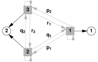
Figure 1: Schematic representation of the hidden Markov process defined by (66–82). The gray squares and gray arrows indicate, respectively, on the realization of the internal Markov process and transitions between the realizations; see (75). The circles and black arrows indicate on the realizations of the observed process. The gray arrows are probabilistic; the corresponding probabilities are indicated next to them. The black arrow are deterministic; see (66).

The process ${\cal X}=\{{\cal X}_{1},{\cal X}_{2},....\}$ has two realizations: ${\cal X}_{i}=1,2$. The corresponding transfer matrices read from (7)

$$T(1)=\left(\begin{array}[]{rrr}1-p_{1}-p_{2}&q_{1}&r_{1}\\ 0{}{}{}{}{}&0&0\\ 0{}{}{}{}{}&0&0\\ \end{array}\right),\qquad T(2)=\left(\begin{array}[]{rrr}0{}{}{}{}{}{}&0{}{}{}{}&0{}{}{}{}{}\\ p_{1}{}{}{}{}{}&1-q_{1}-q_{2}&r_{2}{}{}{}{}{}\\ p_{2}{}{}{}{}{}&q_{2}{}{}{}{}&~{}~{}1-r_{1}-r_{2}\\ \end{array}\right).$$ (82)

Note that the second (sub-dominant) eigenvalue of the transfer-matrix product $\mathbb{T}({\bf x}_{N\ldots 1})=\prod_{k=1}^{N}T(x_{k})$ (with separate transfer-matrices defined by (82)) is equal to zero, since this eigenvalue can be presented as that of the matrix $T(1)A$, where $A$ is some $3\times 3$ matrix. The only exclusion, which has a non-zero sub-dominant eigenvalue, is the realization of ${\cal X}$ that does not contain $1$ at all: $\mathbb{T}(2...2)=T^{N}(2)$.

The considered HMP (66–82) belongs to the class of HMP with unambiguous symbol, since the Markov realization $1$ is not corrupted by the noise; see Fig. 1. For such HMP, Ref. han_markus reports several results on the analytic features of the entropy.

VII.2 Unifilar process.

Before studying in detail the HMP defined by (66–82), let us mention one example of HMP, where the entropy can be calculated directly ash ; ephraim_review . This unifilar process is defined as follows ash : for each realization $s_{i}$ of the Markov process ${\cal S}$ consider realizations $s_{j}$ with a strictly positive transition probability $p(s_{j}|s_{i})>0$. Now require that the realizations $F(s_{j})$ of ${\cal X}_{j}$ are distinct. Thus given the realization $s_{i}$ of ${\cal S}_{1}$, there is one to one correspondence between the realizations of $({\cal X}_{1},{\cal X}_{2},...)$ and those of $({\cal S}_{1},{\cal S}_{2},...)$. Write the block-entropy of ${\cal X}$ as

$$H({\cal X}_{N},...,{\cal X}_{1})=H({\cal X}_{N},...,{\cal X}_{1}|{\cal S}_{1})+H({\cal S}_{1})-H({\cal S}_{1}|{\cal X}_{1},...,{\cal X}_{N}),$$ (83)

where $H({\cal A}|{\cal B})\equiv-\sum_{a,b}{\rm Pr}(a,b)\ln{\rm Pr}(a|b)$ is the conditional entropy of the stochastic variable ${\cal A}$ given ${\cal B}$. Due to the definition of the unifilar process: $H({\cal X}_{N},...,{\cal X}_{1}|{\cal S}_{1})=H({\cal S}_{N},...,{\cal S}_{2}|{\cal S}_{1})$. The latter is worked out via the Markov feature:

$$H({\cal S}_{N},...,{\cal S}_{2}|{\cal S}_{1})=(N-1)h_{\rm markov},$$ (84)

$$h_{\rm markov}=-\sum_{k,l}p_{\rm st}(k)p(l|k)\ln p(l|k),$$ (85)

where $p_{\rm st}(k)$ is the stationary Markov probability defined in (4), and where $p(l|k)$ are the Markov transition probabilities from (3). Since $H({\cal S}_{1})$ and $H({\cal S}_{1}|{\cal X}_{1},...,{\cal X}_{N})$ in (83) are finite in the limit $N\to\infty$, the entropy $h({\cal X})$ of the unifilar process reduces to that of the underlying Markov process $h_{\rm markov}$ ash .

Note that any finite-order Markov process (conventionally assuming that the usual Markov process is of first order) can be presented as a unifilar process. There are, however, unifilar processes that do not reduce to any finite-order Markov process ash   . The main problem in identifying unifilar processes is that even if ${\cal X}$ is not unifilar for given ${\cal S}$, it can be still unifilar with respect to another Markov process ${\cal S}^{\prime}$ (see section VII.3 below for the simplest example). This makes especially difficult the recognition of unifilar processes that do not reduce to any finite-order Markov process.

VII.3 Particular cases.

We now return to the HMP (66–82) and discuss some of its particular cases.

1. For $q_{2}=r_{2}$ and $q_{1}=r_{1}$ all the terms $\varphi_{k}$ with $k\geq 3$ in the expansion (46) are zero. One can check that for this case the observed process ${\cal X}$ is by itself Markov.

2. For $(1-q_{1}-q_{2})(1-r_{1}-r_{2})=q_{2}r_{2}$, one can check that $\phi_{k}=0$ for $k\geq 4$. Now the process ${\cal X}$ is the second-order Markov: $P(x_{k}|x_{k-1},x_{k-2},x_{k-3})=P(x_{k}|x_{k-1},x_{k-2})$.

Thus at least for these two cases the calculation of the entropy is straightforward.

The above two facts tend to clarify the meaning of the expansion (46). It is tempting to suggest that if the expansion (46) is cut precisely at a positive integer $K>2$, i.e., $\varphi_{k\geq K}=0$, then the corresponding process ${\cal X}$ is $K-2$-order Markovian. If true, this will give convenient conditions for deciding on the finite-order Markov feature, and will mean that the successive terms in (46) are in fact approximations the HMP via finite-order Markov processes.

VII.4 Upper and lower bounds for the entropy.

Before presenting the main results of this section, let us recall that the entropy of any (stationary) HMP satisfies the following inequalities cover_thomas :

$$H({\cal X}_{2}|{\cal S}_{1})\leq h\leq H({\cal X}_{2}|{\cal X}_{1})\equiv H(2)-H(1),$$ (86)

where $H({\cal A}|{\cal B})=-\sum_{a,b}{\rm Pr}({\cal A}=a,{\cal B}=b)\ln{\rm Pr}({\cal A}=a|{\cal B}=b)$ and $H(N)$ are, respectively, the conditional entropy and the block entropy defined in (16). Employing (5, 7) we deduce

$${\rm Pr}({\cal X}_{2}=x|{\cal S}_{1}=s)=\sum_{s^{\prime}=1}^{L}T_{s^{\prime}\,s}(x).$$ (87)

This equation together with the stationary probability (75) of the Markov process is sufficient for calculating $H({\cal X}_{2}|{\cal S}_{1})$ for the HMP (66, 82):

$$H({\cal X}_{2}|{\cal S}_{1})=p_{\rm st}(1)\chi(p_{1}+p_{2})+p_{\rm st}(2)\chi(q_{1})+p_{\rm st}(3)\chi(r_{1}),$$ (88)

$$\chi(p)\equiv-p\ln p-(1-p)\ln(1-p).$$ (89)

The upper bound $H({\cal X}_{2}|{\cal X}_{1})$ is calculated directly from (8, 10, 16).

VII.5 Generating function and entropy: exact results.

For a particular four-parametric class of HMP (66–82) we were able to sum exactly the expansion (46) . This class is characterized by the condition that the two leading eigenvalues of the transfer-matrix $T(2)$ in (82) have equal absolute values [the third eigenvalue is equal to zero]:

$$\lambda[T(2)]=\lambda_{1}[T(2)].$$ (90)

A direct inspection shows that this condition amounts to two possible forms (95) and (106) of the transition matrix $\mathbb{P}$. These two cases are studied below.

VII.5.1 First case.

Figure 2: Entropy (100) of HMP (75, 82, 95) versus $q=q_{2}$ for $p_{2}=q_{1}=0$. Normal line: $p_{1}=0.5$. Thick line: $p_{1}=0.75$. Upper dashed line: $p_{1}=0.05$. Lower dashed line: $p_{1}=0.01$. It is seen that for a small value of $p_{1}$, the entropy $h$ is nearly constant for a range of $q=q_{2}$.

For this first case the transition matrix is obtained from (82) under

$$r_{2}=0\quad{\rm and}\quad r_{1}=q_{1}+q_{2}.$$ (91)

This leads from (75) to the transition matrix

$$\mathbb{P}=\left(\begin{array}[]{rrr}1-p_{1}-p_{2}&q_{1}{}{}{}{}&~{}~{}q_{1}+q_{2}{}{}\\ p_{1}{}{}{}{}{}&1-q_{1}-q_{2}&0{}{}{}{}{}\\ p_{2}{}{}{}{}{}&q_{2}{}{}{}{}&~{}~{}1-q_{1}-q_{2}\\ \end{array}\right).$$ (95)

It is seen that the realization $\{{\cal S}_{k+1}=2,\,{\cal S}_{k}=3\}$ for the Markov process is prohibited. For the HMP there are no prohibited sequences.

The inverse zeta-function reads from (46):

$$\xi(z,n) = 1-[\,(1-p_{1}-p_{2})^{n}+(1-q_{1}-q_{2})^{n}\,]\,z$$ (96)

$$+ [\,(1-p_{1}-p_{2})^{n}(1-q_{1}-q_{2})^{n}-(p_{1}q_{1}+p_{2}(q_{1}+q_{2})\,)^{n}\,]z^{2}$$

$$+ z^{3}[p_{1}q_{2}(q_{1}+q_{2})]^{n}\left[\,\Phi(y,-n,b)-\Phi(y,-n,b+1)\,\right],$$

where we defined

$$b\equiv(1-q_{1}-q_{2})\frac{p_{2}(q_{1}+q_{2})+p_{1}q_{1}}{p_{1}q_{2}(q_{1}+q_{2})},$$ (97)

$$y\equiv(1-q_{1}-q_{2})^{n}z,$$ (98)

and where $\Phi(y,-n,b)$ is the Lerch $\Phi$-function:

$$\Phi(y,-n,b)=\sum_{k=0}^{\infty}(k+b)^{n}y^{k}.$$ (99)

In this representation, which led to (96), the sum converges for $|y|<1$ or for $z<(1-q_{1}-q_{2})^{-n}\geq 1$. The convergence radius tends to one for $q_{1}+q_{2}\to 0$, or, equivalently, for $\lambda[T(2)]\to 1$; see (82). This violates the second qualitative condition in (65).

Using (43) we get from (96) for the entropy:

$$h=-\frac{1}{p_{1}+p_{2}+q_{1}+q_{2}+\frac{p_{1}q_{2}}{q_{1}+q_{2}}}\{\,$$

$$(1-p_{1}-p_{2})(q_{1}+q_{2})\ln(1-p_{1}-p_{2})+(1-q_{1}-q_{2})(p_{1}+p_{2}+\frac{p_{1}q_{2}}{q_{1}+q_{2}})\ln(1-q_{1}-q_{2})$$

$$+p_{1}q_{2}\ln[\,p_{1}q_{2}(q_{1}+q_{2})\,]+[\,(p_{1}+p_{2})q_{1}+p_{2}q_{2}\,]\ln[\,(p_{1}+p_{2})q_{1}+p_{2}q_{2}\,]$$

$$+p_{1}q_{2}(q_{1}+q_{2})\left[\,\Phi^{\prime}_{[2]}(1-q_{1}-q_{2},-1,b)-\Phi^{\prime}_{[2]}(1-q_{1}-q_{2},-1,b+1)\,\right]\},$$ (100)

where $b$ is defined in (97), and where

$$\Phi^{\prime}_{[2]}(y,-1,b)=\sum_{k=0}^{\infty}\ln\left[\frac{1}{k+b}\right](k+b)y^{k}.$$ (101)

The behavior of $h$ is illustrated in Fig. 2 for particular values of $p_{1}$, $p_{2}$, $q_{1}$ and $q_{2}$. Table 1 compares the exact expression (100) with the upper and lower bounds (86).

The analytic features of $h$ given by (100) as a function of the Markov transition probabilities $p_{1}$, $p_{2}$, $q_{1}$ and $q_{2}$, agree with the results obtained in han_markus . In particular, note that for $p_{1}+p_{2}\to 1$ the entropy $h$ becomes non-analytic due to the term $\propto(1-p_{1}-p_{2})\ln(1-p_{1}-p_{2})$.

Table 1: For two set of parameters of the HMP (66, 91, 95) we present the exact value of entropy $h$ obtained from (100), the lower bound $H({\cal X}_{2}|{\cal S}_{1})$, and the upper bound $H({\cal X}_{2}|{\cal X}_{1})$; see (86).

	$h$	$H({\cal X}_{2}|{\cal S}_{1})$	$H({\cal X}_{2}|{\cal X}_{1})$
$p_{1}=0.75$
$p_{2}=0.10$	0.569580	0.557243	0.572373
$q_{1}=0.25$
$q_{2}=0.20$
$p_{1}=0.30$
$p_{2}=0.20$	0.684796	0.682486	0.684843
$q_{1}=0.55$
$q_{2}=0.10$

Figure 3: The rate functions $f(\eta)$ and $g(\eta)$ defined by (37) and (39), respectively for the HMP given by (82, 106, 107). Normal line : $g(\eta)$. Dashed line : $f(\eta)$. For the parameters in (106) we take: $p_{1}=0.2$, $p_{2}=0.3$, $q=0.05$, and $r=0.01$. For these values the entropy (108) is $h=0.166671$.

Figure 4: The same as in Fig. 3 but with $q=0.1$ and $r=0.4$. For these values the entropy (108) is $h=0.619519$, which is larger than the entropy in Fig. 3.

VII.5.2 Second case.

The second possibility of satisfying (90) is given by

$$q_{1}+q_{2}=1\quad{\rm and}\quad r_{1}+r_{2}=1,$$ (102)

$$\mathbb{P}=\left(\begin{array}[]{rrr}1-p_{1}-p_{2}&q{}{}{}&r{}{}\\ p_{1}{}{}{}&0{}{}{}&1-r\\ p_{2}{}{}{}&~{}1-q{}{}&0{}{}\\ \end{array}\right).$$ (106)

The realizations of the corresponding Markov process do not contain $\{{\cal S}_{k+1}=2,\,{\cal S}_{k}=2\}$ and $\{{\cal S}_{k+1}=3,\,{\cal S}_{k}=3\}$. Again, the realizations of the HMP do not have any prohibited sequence.

The inverse zeta-function reads from (46)

$$\xi(z,n) = 1-\left[\,(1-p_{1}-p_{2})^{n}+(1-q)^{n/2}(1-r)^{n/2}\,\right]\,z+\left[\,-(p_{1}q+p_{2}r)^{n}+(1-p_{1}-p_{2})^{n}(1-q)^{n/2}(1-r)^{n/2}\,\right]z^{2}$$ (107)

$$+ \frac{z^{3}}{1+z(1-q)^{n/2}(1-r)^{n/2}}\left[\,(p_{1}q+p_{2}r)^{n}(1-q)^{n/2}(1-r)^{n/2}-(\,p_{1}r(1-q)+p_{2}q(1-r)\,)^{n}\,\right].$$

The series that led to (107) converges for $|z|<(1-q)^{-n/2}(1-r)^{-n/2}$. Again the convergence radius going to one violates the second qualitative condition in (65).

Eqs. (32, 107) imply for the source entropy:

$$h=-\frac{1}{\,\,2(p_{1}+p_{2})+q(1-p_{1})+r(1-p_{2})-qr\,\,}\left\{\,[\,q(1-r)+r\,](1-p_{1}-p_{2})\ln(1-p_{1}-p_{2})\right.$$

$$\left.+(p_{1}+p_{2})\,(1-q)\,(1-r)\,\ln[(1-q)(1-r)]+(p_{1}q+p_{2}r)\ln[p_{1}q+p_{2}r]\right.$$

$$\left.+[p_{2}q(1-r)+p_{1}(1-q)r]\ln[p_{2}q(1-r)+p_{1}(1-q)r]\,\right\}.$$ (108)

Applying the general definition (85) of the Markov entropy to the particular case (75) we get for the Markov entropy

$$h_{\rm markov} = -\frac{1}{\,\,2(p_{1}+p_{2})+q(1-p_{1})+r(1-p_{2})-qr\,\,}\,\{\,$$ (109)

$$[\,q(1-r)+r\,][\,(1-p_{1}-p_{2})\ln(1-p_{1}-p_{2})+p_{1}\ln p_{1}+p_{2}\ln p_{2}\,]$$

$$[(1-r)(p_{1}+p_{2})+p_{1}r]\,[q\ln q+(1-q)\ln(1-q)]$$

$$[p_{2}+p_{1}(1-q)]\,[r\ln r+(1-r)\ln(1-r)]\,\}.$$

Comparing (108, 109) one can check [e.g., numerically] that $h_{\rm markov}>h$, as should be, since lumping several states together decreases the entropy. Table 2 compares the exact value (108) for the entropy with the upper and lower bounds (86).

Table 2: For two set of parameters of the HMP (75, 82, 106) we present the exact value of entropy $h$ obtained from (108), the lower bound $H({\cal X}_{2}|{\cal S}_{1})$, and the upper bound $H({\cal X}_{2}|{\cal X}_{1})$; see (86). The parameters $p_{1}$, $p_{2}$, $q$ and $r$ are tuned such that $H({\cal X}_{2}|{\cal S}_{1})$ and $H({\cal X}_{2}|{\cal X}_{1})$ provide rather tight bounds on $h$.

	$h$	$H({\cal X}_{2}|{\cal S}_{1})$	$H({\cal X}_{2}|{\cal X}_{1})$
$p_{1}=0.1$
$p_{2}=0.1$	0.528531	0.525571	0.528534
$q=0.2$
$r=0.3$
$p_{1}=0.2$
$p_{2}=0.2$	0.659897	0.656974	0.659901
$q=0.3$
$r=0.4$

VII.5.3 Rate functions for large deviations.

Recall that the rate function $f(\eta)$ ($g(\eta)$) defined in section V, describe the weight of atypical sequences with the probability smaller (larger) than the typical sequence probability $e^{-Nh}$. The positive parameter $\eta$ defines the amount of this smallness (largeness); see (37) and (39).

The calculation of $f(\eta)$ and $g(\eta)$ for the considered HMP model (106, 82) is straightforward. One finds out the zero of the $\xi$-function given by (107). This will define, via (41), the moment-generating function $\Lambda(n)$. If there are several zeros of $\xi(z,n)$ as a function of $z$, we select the one that goes to $z=1$ for $n\to 1$. Then $f(\eta)$ and $g(\eta)$ are calculated from their definitions (37) and (39).

The behavior of $f(\eta)$ and $g(\eta)$ as functions of $\eta$ is presented in Figs. 3 and 4. For each figure we take different sets of parameters $p_{1}$, $p_{2}$, $q$ and $r$; see (106) for their definition. To make this difference explicit let us denote $f_{3}(\eta)$, $g_{3}(\eta)$ and $f_{4}(\eta)$, $g_{4}(\eta)$ for Fig. 3 and Fig. 4, respectively.

Now let us observe that

$$f_{3}(\eta)<f_{4}(\eta),\qquad g_{3}(\eta)<g_{4}(\eta),$$ (110)

$$g_{3}(\eta)>f_{3}(\eta),\qquad g_{4}(\eta)<f_{4}(\eta).$$ (111)

For explaining these inequalities we note that for the parameters of Fig. 3 the entropy is smaller than $h$ in Fig. 4:

$$h_{3}<h_{4},$$ (112)

which means that the typical set $\Omega_{N}^{*}$ for Fig. 4 contains more sequences, so there remains less of them outside, which may explain (110). For the same reason (112), the probability of each typical sequence is higher for the parameters in Fig. 3. Thus for the parameters presented in Fig. 3 more high-probability sequences are included in the corresponding typical set $\Omega_{N}^{*}$. This may explain (111).

In further numerical checkings it was noted that the above relation between (110) and (111) from one side, and (112) from another side, seems to be much more general than these particular examples.

VIII Binary symmetric Hidden Markov Process.

VIII.1 Definition and symmetries.

This is another popular (and simple to define) example of HMP. Now the Markov process has two states $1$ and $2$. The realizations of the observed (Hidden Markov) process also take two values $1$ and $2$. The internal Markov process is driven by the conditional probability

$$\mathbb{P}=\left(\begin{array}[]{rr}p(1|1){}{}&~{}~{}p(1|2){}{}\\ \\ p(2|1){}{}&~{}~{}p(2|2){}{}\\ \end{array}\right)=\left(\begin{array}[]{rr}1-q&~{}~{}q{}{}\\ \\ q{}{}&~{}~{}1-q\\ \end{array}\right).$$ (119)

The stationary probability for this Markov process is found via (4): $p_{\rm st}(1)=p_{\rm st}(2)=\frac{1}{2}$.

The probabilities for the observations $1$ or $2$ given the internal state read

$$\pi(x_{i}|s_{i})=\left(\begin{array}[]{rr}\pi(1|1){}{}&~{}~{}\pi(1|2){}{}\\ \\ \pi(2|1){}{}&~{}~{}\pi(2|2){}{}\\ \end{array}\right)=\left(\begin{array}[]{rr}1-\epsilon&~{}~{}\epsilon{}{}\\ \\ \epsilon{}{}&~{}~{}1-\epsilon\\ \end{array}\right),$$ (126)

where $\epsilon$ is the error probability during the observation.

For the transfer matrices we have:

$$T(1)=\left(\begin{array}[]{rr}\epsilon(1-q){}{}&~{}~{}\epsilon q{}{}{}{}{}{}{}{}{}\\ \\ (1-\epsilon)q{}{}&~{}~{}(1-\epsilon)(1-q){}{}\\ \end{array}\right),\qquad T(2)=\left(\begin{array}[]{rr}(1-\epsilon)(1-q){}{}&~{}~{}(1-\epsilon)q{}{}\\ \\ \epsilon q{}{}{}{}{}{}{}{}{}&~{}~{}\epsilon(1-q){}{}\\ \end{array}\right).$$ (133)

$T(2)$ is obtained from $T(1)$ via $\epsilon\to 1-\epsilon$.

The following symmetry features are deduced directly from (119–133):

(1) For any $N$ the probability $P(x_{N},\ldots,x_{1};q,\epsilon)$ of the binary symmetric HMP is invariant with respect to $\epsilon\to 1-\epsilon$: $P(x_{N},\ldots,x_{1};q,\epsilon)=P(x_{N},\ldots,x_{1};q,1-\epsilon)$.

(2) The probability $P(x_{N},\ldots,x_{1};q,\epsilon)$ is invariant with respect to the full ”inversion” of the realization $(x_{N},\ldots,x_{1})$, e.g. $P(1,2,1,1;q,\epsilon)=P(2,1,2,2;q,\epsilon)$.

(3) In general, the probability $P(x_{N},\ldots,x_{1};q,\epsilon)$ is not invariant with respect to $q\to 1-q$, e.g., $P(1,2;q,\epsilon)-P(1,2;1-q,\epsilon)=\frac{1}{2}(1-2\epsilon)(2q-1)$. However, for each given realization $(x_{N},\ldots,x_{1})$ one can find another unique realization $(\bar{x}_{N},\ldots,\bar{x}_{1})$ such that $P(x_{N},\ldots,x_{1};q,\epsilon)=P(\bar{x}_{N},\ldots,\bar{x}_{1};1-q,\epsilon)$. The logics of relating $(x_{N},\ldots,x_{1})$ to $(\bar{x}_{N},\ldots,\bar{x}_{1})$ should be clear from the following example: if $(x_{4},\ldots,x_{1})=(1,2,2,1)$, then $(\bar{x}_{4},\ldots,\bar{x}_{1})=(2,2,1,1)$. In more detail, $\bar{x}_{4}=2$ is defined to be different from $x_{4}=1$, and once $x_{3}=2$ is different from $x_{4}=1$, $\bar{x}_{3}=2$ does not differ from $\bar{x}_{4}=2$, etc. It should be clear (e.g., by induction) that for a given $(x_{N},\ldots,x_{1})$, $(\bar{x}_{N},\ldots,\bar{x}_{1})$ is indeed unique.

This feature means, in particular, that the entropy $h$ of the binary symmetric HMP—being according to (16, 17) a symmetric function of all probabilities $P(x_{N},\ldots,x_{1})$—is invariant with respect to $q\to 1-q$: $h(q,\epsilon)=h(1-q,\epsilon)$, in addition to being invariant with respect to $\epsilon\to 1-\epsilon$.

(4) In general, the probabilities $P(x_{N},\ldots,x_{1})$ are not invariant with respect to a cyclic interchange of the realizations, e.g., $P(1,2,1;q,\epsilon)-P(1,1,2;q,\epsilon)=\frac{1}{2}(1-2\epsilon)^{2}q(2q-1)$.

For the considered binary symmetric HMP we did not find any exactly solvable situation. Thus, we employed (46) and calculated $\xi(z,n)$ by approximating the infinite sum in the RHS of (46) via a polynom of order $K$: $\sum_{k=2}^{K}\varphi_{k}(n)z^{k}$   . This approximation was suggested in artuso and it is based on the fact that the sum supposed to converge exponentially at least in the vicinity of $z=1$ and $n=1$. This is what we saw for the exactly solvable situations (96) and (107). The qualitative criterion for the exponential converges was suggested in artuso ; mainieri and was discussed by us around (65). Since both transfer-matrices in (133) have the same eigenvalues

$$\frac{1}{2}\left[\,1-q\pm\sqrt{q^{2}+(1-2q)(1-2\epsilon)^{2}}\,\right],$$ (134)

for the studied binary symmetric HMP there are several cases, where the [qualitative] conditions (65) are violated: i) $q\to 0$ and $\epsilon\to\frac{1}{2}$; ii) $q\to 1$; iii) $q\to 0$ and $\epsilon\to 0$. In these three cases we expect that that approximating $\xi(z,n)$ by $\sum_{k=2}^{K}\varphi_{k}(n)z^{k}$ will not be feasible, since large values of $K$ will be required to achieve a reasonably high precision. Fig. 5 and Table 3 present the results for the entropy obtained in the above approximate way and compare them with the upper and lower bounds, as given by (86).

Table 3: For two sets of the parameters $q$ and $\epsilon$ of the binary symmetric HMP (119, 126, 133) we present the entropy $h$ obtained by approximating (46) via a polynomial or order $2$, $13$ and $12$, respectively. These values are denoted by $h_{2}$, $h_{13}$ and $h_{12}$. We compare $h_{k}$ with the lower bound $H({\cal X}_{2}|{\cal S}_{1})$, and the upper bound $H({\cal X}_{2}|{\cal X}_{1})$; see (86). It is seen that the relative difference $\frac{h_{13}-h_{2}}{h_{13}}$ is not larger than $0.02$.

	$h_{2}$	$h_{13}$	$h_{12}$	$H({\cal X}_{2}|{\cal S}_{1})$	$H({\cal X}_{2}|{\cal X}_{1})$
$q=0.2$
$\epsilon=0.45$	0.687811	0.693108	0.693100	0.691346	0.693129
$q=0.25$
$\epsilon=0.4$	0.681322	0.692884	0.692881	0.688139	0.692947

Figure 5: Entropy of the binary hidden Markov chain (normal line) versus the error probability $\epsilon$ for $q=0.1$. Dashed lines: upper and lower bounds for the entropy as given by (86). The entropy is calculated from (46, 43) approximating the infinite sum in (46) by a poynomial or the order $13$.

VIII.2 Small-noise limit.

For $\epsilon=\frac{1}{2}$ or for $q=\frac{1}{2}$ the process becomes memory-less: $P(x_{1},...,x_{N})=P(x_{1})...P(x_{N})$. Here all the functions $\varphi_{k}$ in (46) are equal to zero. Another particular case is the limit $\epsilon\to 0$ (no noise), where the hidden Markov process degenerates into the original Markov process. It is straightforward to check that in (46) for the entropy only the term $\phi_{2}$ is different from zero, while $\phi_{k}=0$ for $k\geq 3$. This produces the well-known expression (85) for the entropy of a Markov process.

Let us work out the vicinity of $\epsilon=0$, assuming that $\epsilon$ is small (quasi-Markov situation). One can check that

$$\varphi_{k}={\cal O}(\epsilon^{k-2})\qquad{\rm for}\qquad k\geq 3.$$ (135)

Thus for finding the entropy and the generating function within the order ${\cal O}(\epsilon^{2})$, we need to expand $\varphi_{k}$ with $k=1,2,3,4$ over $\epsilon$ and select all the terms of order ${\cal O}(\epsilon)$ and ${\cal O}(\epsilon^{2})$. We write down explicitly the approximation of $\xi(z,n)$ via the polynom of order $4$ (higher-order terms $\varphi_{k\geq 5}$ are not needed, since they do not contribute to the order ${\cal O}(\epsilon^{2})$):

$$\xi(z,n)=1+z\,\varphi_{1}(n)+z^{2}\varphi_{2}(n)+z^{3}\varphi_{3}(n)+z^{4}\varphi_{4}(n)+{\cal O}(z^{3}).$$ (136)

Using (134) and (50–53) we get after straightforward algebraic calculations (taking for simplicity $q<\frac{1}{2}$)

$$\varphi_{1}(n) = -2\,{\left(1-q\right)}^{n}$$ (137)

$$+ 2\,\epsilon\,n\,{\left(1-q\right)}^{n-2}\,\left(1-2\,q\right)$$

$$- \epsilon^{2}\,n\,{\left(1-q\right)}^{n-4}\,\left(1-2\,q\right)\,\left\{\,(1-2q)(n-1-q)+q\,\right\}+{\cal O}(\epsilon^{3}),$$

$$\varphi_{2}(n) = {\left(1-q\right)}^{2\,n}-q^{2\,n}$$ (138)

$$- 2\,\epsilon\,n\,\left(1-2\,q\right)\,\left[{\left(1-q\right)}^{2\,\left(n-1\right)}+q^{2\,(n-1)}\right]$$

$$- \epsilon^{2}\,n\,\left(1-2\,q\right)\,\left[q^{2\,(n-2)}\,\left\{\,(1-2q)(q+2n-3)-q\,\right\}\right.$$

$$~{}~{}~{}~{}~{}~{}~{}~{}~{}~{}~{}~{}~{}~{}~{}~{}~{}\left.+(1-q)^{2(n-2)}\,\left\{\,(1-2q)(q+1-2n)-q\,\right\}\right]+{\cal O}(\epsilon^{3}),$$

$$\varphi_{3}(n) = 2\epsilon\,n\,(1-2q)^{2}\,(1-q)^{n-2}\,q^{2(n-1)}$$ (139)

$$- \epsilon^{2}\,n\,(1-2q)^{2}\,(1-q)^{n-4}\,q^{2(n-2)}\,\left[\,5-3n+4q(3n-5)+2q^{2}(16-7n)\right.$$

$$~{}~{}~{}~{}~{}~{}~{}~{}~{}~{}~{}~{}~{}~{}~{}~{}~{}~{}~{}~{}~{}~{}~{}~{}~{}~{}~{}~{}~{}~{}~{}~{}~{}~{}~{}~{}~{}~{}~{}~{}~{}~{}\left.+4q^{3}(n-6)+10q^{4}\,\right]+{\cal O}(\epsilon^{3}),$$

$$\varphi_{4}(n)=\epsilon^{2}n\,(1-2q)^{3}\,(1-q)^{2(n-2)}\,q^{2(n-2)}\,\left[\,2-4q(1-q)-n(1-2q)\,\right]+{\cal O}(\epsilon^{3}).$$ (140)

Note that all $\epsilon$ corrections nullify for $q=\frac{1}{2}$, once in this limit we should get a memory-less process. These equations produce for the entropy from (136, 43):

$$h = -(1-q)\ln(1-q)-q\ln q$$ (141)

$$- 2\epsilon\,(1-2q)\,\ln\left(\frac{1-q}{q}\right)$$ (142)

$$- 2\epsilon^{2}\,(1-2q)\left[\,\ln\left(\frac{1-q}{q}\right)+\frac{1-2q}{4(1-q)^{2}\,q^{2}}\,\right]+{\cal O}(\epsilon^{3}).$$ (143)

Eq. (141) is just the Markov entropy (85) obtained in the limit $\epsilon=0$. Eqs. (142) is the first correction to the Markov situation; it is obtained in jacquet ; weissman . The second correction (143) is reported in zuk_jsp . The authors of zuk_jsp also obtain the higher-order corrections employing the mapping of the binary symmetric HMP to the one-dimensional Ising model. These higher-order correction can be also obtained within the present method. Thus we demonstrated that the small-noise (quasi-Markov) situation can be adequately explored with the present method.

In addition we obtain the small-noise expressions (137-140) for the zeta-function. This result is new and it allows to find the moment-generating function, which contains more information than the entropy, e.g., (136–140) can be used for approximating the rate functions (37) and (39). In particular, for the generating function we get from (41) and (137–140)

$$\Lambda(n)=q^{n}+(1-q)^{n}-\frac{\epsilon n(1-2q)\left[\,(1-q)^{2n}q^{2}-(1-q)^{2}q^{2n}\,\right]}{q^{2}(1-q)^{2}\left[\,(1-q)^{n}+q^{n}\,\right]}+{\cal O}(\epsilon^{2}).$$ (144)

IX Summary.

In this paper we studied the entropy and the moment-generating function of Hidden Markov Processes (HMP). The fact that these processes model non-Markov memory is at the origin of their numerous applications, and, simultaneously, the main reason of difficulties in characterizing their entropy and the moment-generating function. Recall that the entropy gives the number of sequences in the typical set of the random process cover_thomas ; strat ; the typical set is the smallest set of realizations with the overall probability close to one. Alternatively, the entropy is the uncertainty [per time-unit] of the process given its long history. The generating function allows to estimate the [small] probability of atypical sequences via the Chernoff bound and the rate functions cover_thomas ; strat . The entropy of HMP was studied via upper and lower bounds cover_thomas ; birch , expansions over small parameters zuk_jsp ; zuk_aizenman ; chigan , and via expressing the entropy as a solution of an integral equation strat ; blackwell ; birch ; jacquet ; gold ; weissman ; egner .

Here we proposed to calculate the entropy and the moment-generating function of HMP via the cycle expansion of the zeta-function, a method adopted from the theory of dynamical systems artuso ; mainieri ; gaspar . I show that this method has two basic advantages. First, it produces exact results, both for the entropy and the moment-generating function, for a class of HMP. We did not so far got into any systematic way of searching for the exact solutions within this method. The examples of exact solutions presented in section VII.5 were obtained in the most straightforward way. Second, even if no exact solution is found, the method offers an expansion for the entropy and the moment-generating function via an exponentially convergent power series artuso ; mainieri ; gaspar . Cutting off these expansions at some finite order gives normally an improvable approximation for the sought quantities, especially since there are qualitative estimates for the convergence radius of the series. This was demonstrated in section VIII.

As a by-product of this study, we conjectured in section VII.3 on tentative conditions under which HMP reduces to a finite-order Markov process. These conditions compare favorably with those existing in literature, see e.g. lolo , and they deserve further exploration. We also conjectured relations (110–112) between the rate functions of the random process and its entropy.

Appendix A Recollection of some facts about the eigen-representation versus singular value decomposition.

A matrix $A$ can be diagonalized if horn

$$A=V\,D\,V^{-1},$$ (145)

where $D$ is a diagonal matrix, and where $V$ is an arbitrary invertible matrix. Writing the eigen-resolution of $D$, $D=\sum_{k}\alpha_{k}|\alpha_{k}\rangle\langle\alpha_{k}|$, where $\langle\alpha_{k}|\alpha_{n}\rangle=\delta_{kn}$, one gets

$$A=\sum_{k}\alpha_{k}|R_{k}\rangle\langle L_{k}|,$$ (146)

where $\alpha_{k}$ are the eigenvalues of $A$ (i.e., the solutions of ${\rm det\,}(A-\alpha\,1)=0$), and where $|R_{k}\rangle$ and $|L_{k}\rangle$ are, respectively, the right and left eigenvectors:

$$A|R_{k}\rangle=\alpha_{k}|R_{k}\rangle,\qquad\langle L_{k}|A=\alpha_{k}\langle L_{k}|,\qquad\langle L_{k}|R_{n}\rangle=\delta_{kn}.$$ (147)

Note that in general $\langle L_{k}|L_{n}\rangle\not=\delta_{kn}$. The right and left eigenvectors coincide for normal matrices $[A,A^{\dagger}]=0$ ($A$ commutes with its complex conjugate). For those matrices $V$ is unitary.

Not every matrix can be diagonalized, a necessary and sufficient condition for this is that for each eigenvalue the algebraic degeneracy (i.e., degeneracy of this eigenvalue as the root of the characteristic polynom) coincides with the geometric degeneracy (the number of eigenvectors corresponding to this eigenvalue; geometric degeneracy cannot be larger than the algebraic one). Thus a sufficient condition for a matrix to be diagonalizable is that its eigenvalues are not degenerate. Here is a more general sufficient condition: Any matrix that commutes with a matrix with non-degenerate eigenvalues, is diagonalizable horn .

If for one eigenvalue $\alpha$ of $A$ the algebraic and geometric degeneracies are equal (say to $m$), then

$$A=V\left(\begin{array}[]{rr}\alpha I_{m\times m}{}{}&~{}~{}0{}{}\\ 0{}{}&~{}~{}A^{\prime}{}{}\\ \end{array}\right)V^{-1},$$ (150)

where $I_{m\times m}$ is the $m\times m$ unit matrix.

An alternative representation for the matrix $A$ is given by the singular value decomposition. Note that if ${\rm det}\,\,A\not=0$, the matrix $A[A^{\dagger}A]^{-1/2}$ is unitary. Then it holds

$$A=U\,[A^{\dagger}A]^{1/2},$$ (151)

where $U$ is unitary. Eq. (151) holds also for ${\rm det}\,A=0$ via the continuity. Going to the eigen-resolution of the hermitian matrix $A^{\dagger}A$, we see that for any matrix $A$ there is a singular value decomposition:

$$A=\sum_{k}\sigma_{k}|u_{k}\rangle\langle v_{k}|,$$ (152)

$$A|v_{k}\rangle=\sigma_{k}|u_{k}\rangle,\qquad\langle v_{k}|v_{n}\rangle=\delta_{kn}$$ (153)

$$\langle u_{k}|A=\sigma_{k}\langle v_{k}|,\qquad\langle u_{k}|u_{n}\rangle=\delta_{kn},$$ (154)

where $\sigma_{k}$ (singular values of $A$) is the common eigenvalue spectrum of $\sqrt{AA^{\dagger}}$ and $\sqrt{A^{\dagger}A}$.

For a given diagonalizable matrix $A$, its singular value decomposition is related to the eigen-resolution via horn

$$\langle v_{n}|R_{k}\rangle\sigma_{n}=\alpha_{k}\langle u_{n}|R_{k}\rangle,$$ (155)

$$\langle u_{n}|L_{k}\rangle\sigma_{n}=\alpha_{k}^{*}\langle v_{n}|L_{k}\rangle.$$ (156)

The matrix $A$ is normal if and only if $|\alpha_{k}|=\sigma_{k}$. (I did not find any standard reference on the fact that $|\alpha_{k}|=\sigma_{k}$ leads to normality; the proof I got myself is too tedious to be presented here).

Singular values and eigenvalues are related via the Weyl inequalities. For a given matrix $A$, order the absolute values of its eigenvalues as $l_{0}\geq l_{1}\geq...\geq l_{n}$, and order its singular values as $\sigma_{0}\geq\sigma_{1}\geq...\geq\sigma_{n}$. The Weyl inequalities then read:

$$\prod_{k=0}^{m}\sigma_{k}\geq\prod_{k=0}^{m}l_{k},\quad\prod_{k=0}^{m}\sigma_{n-k}\leq\prod_{k=0}^{m}l_{n-k},$$ (157)

$$\sum_{k=0}^{m}\sigma_{i}^{\rho}\geq\sum_{k=0}^{m}l_{i}^{\rho},\qquad\rho>0.$$ (158)

For $n=m$, (157) leads to equality: $\prod_{k=0}^{n}\sigma_{k}=\prod_{k=0}^{n}l_{k}$.

Appendix B Additional features of the entropy.

Recall the definitions (17) and (16) of the entropy $h$ and the block entropy $H(N)=H({\cal X}_{N},...,{\cal X}_{1})$, respectively, for the stationary process ${\cal X}$. Define:

$$h(N)=H(N)-H(N-1)=H({\cal X}_{N}|{\cal X}_{N-1},...,{\cal X}_{1}).$$ (159)

$h(N)$ [sometimes called innovation entropy] is the uncertainty of ${\cal X}_{N}$ given its history ${\cal X}_{N-1},...,{\cal X}_{1}$. It is clear that once ${\rm lim}_{N\to\infty}\frac{H(N)}{N}$ exists, $h(N)$ converges to the source entropy for $N\to\infty$. One can show that cover_thomas

$$\frac{H(N)}{N}\geq h(N)\geq h(N+1)\geq h.$$ (160)

To derive the second inequality in (160) note that the stationarity and the entropy reduction due to conditioning imply

$$h(N)=H({\cal X}_{N}|{\cal X}_{N-1},...,{\cal X}_{1})=H({\cal X}_{N+1}|{\cal X}_{N},...,{\cal X}_{2})\geq H({\cal X}_{N+1}|{\cal X}_{N},...,{\cal X}_{1})=h(N+1).$$ (161)

The first inequality in (160) is shown as follows.

$$\frac{H(N)}{N}=\frac{1}{N}H({\cal X}_{1})+\frac{1}{N}\sum_{i=2}^{N}H({\cal X}_{i}|{\cal X}_{i-1},...,{\cal X}_{1})\geq\frac{1}{N}\sum_{i=1}^{N}H({\cal X}_{N}|{\cal X}_{N-1},...,{\cal X}_{1})=h(N),$$ (162)

where the first equality is the obvious chain rule for the conditional information, while the second inequality in (162) follows from the stationarity $H({\cal X}_{1})=H({\cal X}_{N})$, and then from the same reasoning as in (161). The last inequality in (160) is now obvious.

The meaning of $\frac{H(N)}{N}\geq h\equiv{\rm lim}_{N\to\infty}\frac{H(N)}{N}$ is that taking into account all the correlations decreases the entropy. In a related context, $h(N)\geq h(N-1)$ means that the innovations decrease under accumulation of experience. This inequality can be employed for putting an upper bound for $H(N+1)$ in terms of $H(N)$ and $H(N-1)$:

$$2H(N)-H(N-1)\geq H(N+1)\geq H(N).$$ (163)

Note also that $H(N+1)=H(N)+h(N+1)\leq H(N)+\frac{H(N+1)}{N+1}$ leads to

$$\frac{H(N+1)}{N+1}\leq\frac{H(N)}{N},$$ (164)

i.e., the uncertainty per step decreases when increasing $N$.

Appendix C Ergodic features of the singular values for a random matrix product.

Let us recall some important features of the Lyapunov exponents of the random matrix product (8). Employ the known relation between the singular values of $AB$ versus those of $A$ and $B$ horn

$$\prod_{k=0}^{m}\sigma_{k}[AB]\leq\prod_{k=0}^{m}\sigma_{k}[A]\sigma_{k}[B],$$ (165)

where $0\leq m\leq L-1$, and where the ordering (15) is assumed: $\sigma_{0}[A]\geq\sigma_{1}[A]\geq\ldots$.

Now recall definitions (9, 10). Applying (165) with $m=0$ to $\mathbb{T}({\bf x}_{N\ldots 1})$ we get ($M<N$)

$$\ln\sigma_{0}[\mathbb{T}({\bf x}_{N\ldots 1})]\leq\ln\sigma_{0}[\mathbb{T}({\bf x}_{M-1\ldots 1})]+\ln\sigma_{0}[\mathbb{T}({\bf x}_{N\ldots M})].$$ (166)

Thus, $\ln\sigma_{0}[\mathbb{T}({\bf x}_{N\ldots 1})]$ is sub-additive. Together with the assumptions i), ii) and iii) of section IV.1, Eq. (166) ensures the applicability of the sub-additive ergodic theorem kingman ; steele . This leads (for $N\to\infty$) to the probability-one convergence (24):

$$-\frac{1}{N}\ln\sigma_{k}[\mathbb{T}({\bf x}_{N\ldots 1})]\to\mu_{k},$$ (167)

for $k=0$. Applying in the same way (165) with $m=1$ to $\mathbb{T}({\bf x}_{N\ldots 1})$, we use the sub-additivity for $\ln\left(\sigma_{0}[\mathbb{T}({\bf x}_{N\ldots 1})]\sigma_{1}[\mathbb{T}({\bf x}_{N\ldots 1})]\right)$, deduce (24) for $k=1$, and so on. It is clear that we could not employ the sub-additivity directly for $l_{k}[\mathbb{T}({\bf x}_{N\ldots 1})]$ (modules of the eigenvalues), since they in general do not satisfy to anything like (165).

The sub-additive ergodic theorem is related to the additive (Birkhoff-Khinchin) ergodic theorem that claims the existence (with probability one) of a similar limit for a function $\frac{1}{N}\sum_{k=1}^{N}f[{\cal X}_{k}]$ of the stationary random process ${\cal X}=\{{\cal X}_{1},\ldots,{\cal X}_{N},\ldots\}$ steele .

Appendix D Eigenvalues and singular values of the random matrix product.

Recall section IV.2 and the main question posed there: when the modules of the eigenvalues of the matrix product $\mathbb{T}({\bf x}_{N\ldots 1})$ are equal, for $N\gg 1$, to the singular values of $\mathbb{T}({\bf x}_{N\ldots 1})$.

As shown by (25), for $N\gg 1$ we can keep the dependence on $N$ only in the singular values of $\mathbb{T}$. (We simplified notations as $\mathbb{T}({\bf x}_{N\ldots 1})=\mathbb{T}$.) First assume that $\mathbb{T}$ is a $2\times 2$ matrix. Write the singular value decomposition (151) for $\mathbb{T}$ as

$$\mathbb{T}=\left(\begin{array}[]{rr}e^{-N\mu_{0}}&0{}{}\\ \\ 0{}{}{}{}&e^{-N\mu_{1}}\\ \end{array}\right)U,\qquad U=\left(\begin{array}[]{rr}a&b\\ \\ c&d\\ \end{array}\right),$$ (174)

where $e^{-N\mu_{0}}$ and $e^{-N\mu_{1}}$ [with $\mu_{0}<\mu_{1}$] are the singular values of $\mathbb{T}$, and where the matrix $U$ can be taken real, since $\mathbb{T}$ is real. Thus $U$ is orthogonal: $ab+cd=0$, $a^{2}+c^{2}=b^{2}+d^{2}=1$, $ad-bc=\pm 1$.

For the modules of the eigenvalues of $\mathbb{T}$ in (174) one finds

$$l_{0}=|a|e^{-N\mu_{0}}+\frac{|bc|}{|a|}e^{-N(\mu_{1}-\mu_{0})}+\ldots,\qquad l_{1}=\frac{1}{|a|}e^{-N\mu_{1}}-\frac{2|bc|}{|a|^{3}}\,e^{-N(2\mu_{1}-\mu_{0})}+\ldots.$$ (175)

If $|a|\not=0$, the singular values of $\mathbb{T}$ coincide with the absolute values of its eigenvalues for $N\gg 1$ or : the terms ${\cal O}(e^{-N(\mu_{1}-\mu_{0})})$ and ${\cal O}(e^{-N(2\mu_{1}-\mu_{0})})$ are negligible and $\ln|a|$ is also neglected inside of the exponents as compared to $N\mu_{0}$ and $N\mu_{1}$.

This conclusion changes for $a=0$ (and thus $d=0$ since $U$ is orthogonal). Now the modules of the eigenvalues coincide with each other and are equal to $e^{-N(\mu_{1}+\mu_{2})/2}$ which is different from the singular values.

The next example is $3\times 3$ matrix $\mathbb{T}$ with the determinant equal to zero:

$$\mathbb{T}=\left(\begin{array}[]{rrr}e^{-N\mu_{0}}&0{}{}&0{}{}\\ \\ 0{}{}{}{}&e^{-N\mu_{1}}&0{}{}\\ \\ 0{}{}{}{}&0{}{}&0{}{}\\ \end{array}\right)U,\qquad U=\left(\begin{array}[]{rrr}a&b&e\\ \\ c&d&f\\ \\ x&y&z\end{array}\right),$$ (186)

where $e^{-N\mu_{0}}$ and $e^{-N\mu_{1}}$ [with $\mu_{0}<\mu_{1}$] are two non-zero singular values of $\mathbb{T}$, and where the matrix $U$ is orthogonal. Note that provided the third Lyapunov exponent $\mu_{2}$ is larger than $\mu_{1}$ (and provided we do not use the orthogonality features of the matrix $U$ in (186)), the considered example is sufficiently general.

Since ${\rm det}\,\mathbb{T}=0$, the third singular value of $\mathbb{T}$ is zero. The third eigenvalue of $\mathbb{T}({\bf x}_{N\ldots 1})$ is also equal to zero, while for the absolute values of the remaining eigenvalues we have from (186)

$$l_{0}=|a|e^{-N\mu_{0}}+{\cal O}(\frac{1}{|a|}\,e^{-N(\mu_{1}-\mu_{0})}),\qquad l_{1}=\frac{|ad-bc|}{|a|}e^{-N\mu_{1}}+{\cal O}(e^{-N(2\mu_{1}-\mu_{0})}).$$ (187)

If $|ad-bc|\not=0$, the singular values $e^{-N\mu_{0}}$ and $e^{-N\mu_{1}}$ coincide [for $N\gg 1$] with the modules of the eigenvalues. For $|ad-bc|=0$ the second eigenvalue of $\mathbb{T}$ is equal to zero, while the second singular value is non-zero. However, the first Lyapunov exponent is still equal to the spectral radius (module of the first eigenvalue) if $a\not=0$. The latter two quantities are not equal for $a=0$. Now the modules of both eigenvalues of $\mathbb{T}({\bf x}_{N\ldots 1})$ reduce to $\sqrt{|bc|}\,e^{-N(\mu_{1}+\mu_{2})/2}$.

Using the examples (174, 186) we got a sufficient condition for deciding whether the maximal singular value of $\mathbb{T}$ is equal to the module of the corresponding eigenvalue. It is that the absolute values of the two leading eigenvalues of $\mathbb{T}$ are different.

Appendix E Zeta-function and periodic orbit expansion.

E.1 Structure of periodic orbits.

Define formally

$$Z_{m}=\sum_{i_{1},...,i_{m}=1}^{M}\phi[A_{i_{1}}...A_{i_{m}}],$$ (188)

where $A_{1},...,A_{M}$ are matrices, and where $\phi[.]$ is a function that turn its matrix argument to a number. We assume that the following features hold for $\phi$ ($d$ is a positive integer):

$$\phi[A^{d}]=\phi^{d}[A],\qquad\phi[AB]=\phi[BA].$$ (189)

Using these features one can prove for $Z_{m}$ the following formula ruelle :

$$Z_{m}=\sum_{n|m}\,\,\,\sum_{(\gamma_{1},...,\gamma_{n})\in{\rm Per}(n)}n\left[\,\phi[A_{\gamma_{1}}...A_{\gamma_{n}}]\,\right]^{\frac{m}{n}},$$ (190)

where $\sum_{n|m}$ means that the summation goes over all $n$ that divide $m$, e.g., $n=1,2,4$ for $m=4$. Here ${\rm Per}(n)$ contains sequences

$$\Gamma=(\gamma_{1},...,\gamma_{n})$$ (191)

selected according to the following rules: i) $\Gamma$ turns to itself after $n$ successive cyclic permutations, but does not turn to itself after any smaller (than $n$) number of successive cyclic permutations; ii) if $\Gamma$ is in ${\rm Per}(n)$, then ${\rm Per}(n)$ contains none of those $n-1$ sequences obtained from $\Gamma$ under $n-1$ successive cyclic permutations.

Assume that $M=2$, which means that the matrices $A_{i}$ can take two values $A_{1}=1$ and $A_{2}=2$. With examples of ${\rm Per}(n)$ given in Table 4, the proof of (190) is straightforward.

Table 4: The elements of ${\rm Per}(p)$ for $p=1,...,5$ and $M=2$. As compared to (9) we denoted $T(x_{1})=1$ and $T(x_{2})=2$. It is seen that ${\rm Per}(1)$ contains two elements, since the cyclic permutation is trivial. ${\rm Per}(2)$ contains a single element $12$, since $11$ and $22$ remain invariant under a single cyclic permutation, while $BA$ is obtained from $AB$ via a single cyclic permutation. Besides the obvious sequences $1111$ and $2222$, ${\rm Per}(4)$ does not include the sequences $1212$ and $2121$ which stay invariant after two successive cyclic permutations. In ${\rm Per}(5)$ we first meet different elements that have the same overall number of $1$’s and $2$’s, e.g., $12121$ and $11122$.

$p$	${\rm Per}(p)$
$1$	$1$, $2$
$2$	$12$
$3$	$122$, $211$
$4$	$1222$, $2111$, $1122$
$5$	$12222$, $21111$, $11222$,
	$22111$, $12121$, $21212$
$6$	$122222$, $112222$, $111222$,
	$111122$, $111112$,
	$112212$, $221121$
	$111212$, $222121$.

Table 5: The elements of ${\rm Per}(p)$ for $p=1,...,4$ and $M=3$.

$p$	${\rm Per}(p)$
$1$	$1,2,3$
$2$	$12$, $13$, $23$
$3$	$122$, $211$, $233$
	$322$, $133$, $311$
	$123$, $132$
$4$	$1222$, $2111$, $1122$,
	$2333$, $3222$, $2233$
	$1333$, $3111$, $1133$
	$1123$, $1132$, $1213$
	$2213$, $2231$, $2321$
	$3312$, $3321$, $3231$

E.2 The inverse zeta-function and derivation of Eq. (44).

The inverse zeta function is defined as $\xi(z)=\exp\left[-\sum_{m=1}^{\infty}\frac{z^{m}}{m}Z_{m}\right]$, where $Z_{m}$ is given by (188). Employing (190) and introducing notations $p=n$, $q=\frac{m}{n}$, we transform $\xi(z)$ as

$$\xi(z)=\exp\left[\,-\sum_{p=1}^{\infty}\,\sum_{\Gamma\in{\rm Per}(p)}\,\sum_{q=1}^{\infty}\frac{z^{pq}}{q}\left(\phi[A_{\gamma_{1}}...A_{\gamma_{p}}]\,\right)^{q}\right].$$ (192)

the summation over $q$ in (192) is taken as

$$\sum_{q=1}^{\infty}\frac{z^{pq}}{q}\left(\phi[A_{\gamma_{1}}...A_{\gamma_{p}}]\,\right)^{q}=-\ln\left[1-z^{p}\phi[A_{\gamma_{1}}...A_{\gamma_{p}}]\,\right].$$ (193)

We shall then finally get artuso ; ruelle :

$$\xi(z)=\prod_{p=1}^{\infty}\,\prod_{\Gamma\in{\rm Per}(p)}\,\left[1-z^{p}\phi[A_{\gamma_{1}}...A_{\gamma_{p}}]\,\right].$$ (194)

E.3 How to generate the elements of ${\rm Per}(p)$ via Mathematica 5.

The elements of ${\rm Per}(p)$ presented in Tables 4 and 5 were generated by hands. For larger $p$ it is more convenient to generate these elements via Mathematica 5. Below we assume that the reader knows Mathematica at some average level. First one should run the package of combinatoric functions:

<<DiscreteMath‘Combinatorica‘ (195)

Next one defines the function ListNecklaces2[c_List, n_Integer?Positive] list , the first argument of which is a list, e.g., { A,B } , while the second argument is a positive integer.

AllCombinations[x_List, n_Integer?NonNegative]

:= Flatten[Outer[List, Sequence Table[x, {n}]], n - 1];

ListNecklaces2[c_List, n_Integer?Positive] := Module[{},

Return[OrbitRepresentatives[CyclicGroup[n], AllCombinations[c, n]]]]; (196)

The definition of ListNecklaces2 proceeds via an auxiliary function AllCombinations. All other functions in (196) are contained in the package (195).

Upon running ListNecklaces2[c, p] one gets the elements of ${\rm Per(p)}$ together with those sequences $(\gamma_{1},...,\gamma_{p})$ that remain invariant under $\bar{p}$ successive cyclic permutation, where $p/\bar{p}$ is an integer. For our purposes we meed only the sequences which are invariant with respect to $p$ cyclic permutation, and are not variant with respect to cyclic permutations with any smaller $\bar{p}$. So our next task is to get rid of those parasitic sequences, which stay invariant with respect to $\bar{p}$ cyclic permutations with $\bar{p}<p$. To this end we designed a straightforward Mathematica program that by the direct enumeration detects and eliminates the parasitic sequences [obviously, nothing special has to be done for simple numbers like $p=3,5,7,11,13$]. The drawback of this program is that for each $p$ in ${\rm Per}(p)$ one has to adjust the details of this program. Anyhow, we were not able to enforce Mathematica 5 to generate the elements of ${\rm Per}(p)$ directly.

Here is an example of the above scheme: ListNecklaces2[{A,B}, 3] generates a list of lists:

$$\texttt{\{ \{ A,A,A \}, \{ A,A,B\}, \{ A,B,B\}, \{ B,B,B\} \}}.$$ (197)

After elimination of the parasitic sequences this results in

$$\texttt{Y}=\texttt{\{ \{ A,A,B\}, \{ A,B,B\} \}},$$ (198)

where we introduced a shorthand Y. Now employing the construction

$$\texttt{ Apply[Times, Map[ f[\#] \&, Apply[Dot, Y, 1] ] ] },$$ (199)

where f is an arbitrary function, one gets

$$\texttt{f[A.A.B] f[A.B.B]}.$$ (200)

The construction (199) is useful when recovering the formulas for $\phi_{k}$ for large values of $p$.

References

• (1) L. R. Rabiner, Proc. IEEE, 77, 257-286, (1989).
• (2) Y. Ephraim and N. Merhav, IEEE Trans. Inf. Th., 48, 1518-1569, (2002).
• (3) M. Crouse, R. Nowak and R. Baraniuk, IEEE Tran. Signal Process., 46, 886 (1998).
• (4) T. Koski, Hidden Markov Models for Bioinformatics (Kluwer, Academic Publishers, Dordrecht, 2001). P. Baldi and S. Brunak, Bioinformatics (MIT Press, Cambridge, USA, 2001).
• (5) R. Ash, Information Theory (Interscience Publishers, NY, 1965).
• (6) T. M. Cover and J. A. Thomas, Elements of Information Theory, (Wiley, New York, 1991).
• (7) D. Blackwell, The entropy of functions of finite-state markov chains, in Trans. First Prague Conf. Inf. Th., Statistical Decision Functions, Random Processes, p. 13 (Pub. House Chechoslovak Acad. Sci., Prague, Czechoslovakia, 1957).
• (8) R.L. Stratonovich, Information Theory (Sovietskoe Radio, Moscow, 1976) (In Russian).
• (9) M. Rezaeian, Hidden Markov Process: A New Representation, Entropy Rate and Estimation Entropy, arXiv:cs.IT/0606114.
• (10) I.J. Birch, Ann. Math. Stat. 33, 930 (1962).
• (11) P. Jacquet, G. Seroussi, and W. Szpankowski, On the Entropy of a Hidden Markov Process, Int. Symp. Inf. Th. p. 10, Chicago, IL, 2004.
• (12) T. Holliday, A. Goldsmith and P. Glynn, IEEE Trans. Inf. Th. 52, 3509 (2006).
• (13) E. Ordentlich and T. Weissman, IEEE Trans. Inf. Th., 52, 19 (2006).
• (14) S. Egner et al., On the Entropy Rate of a Hidden Markov Model, Int. Symp. Inf. Th., p. 12, Chicago, IL (2004).
• (15) O. Zuk, I. Kanter and E. Domany, J. Stat. Phys. 121, 343 (2005).
• (16) O. Zuk, I. Kanter, E. Domany and M. Aizenman, IEEE Signal Processing Letters, 13, 517 (2006).
• (17) P.Chigansky, The Entropy Rate of a Binary Channel with Slolwly Varying Input, arXiv:cs/0602074.
• (18) R. A. Horn and C. R. Johnson, Matrix Analysis (Cambridge University Press, New Jersey, USA, 1985).
• (19) J.F.C. Kingman, Ann. Probab. 1, 883 (1973).
• (20) J.M. Steele, Annales de l’I.H.P. B, 25, 93 (1989).
• (21) A. Crisanti, G. Paladin and A. Vulpiani, Products of Random Matrices in Statistical Physics, Springer Series in Solid State Sciences, Vol. 104, (Springer, Berlin, 1993).
• (22) L.Y. Goldsheid and G.A. Margulis, Russ. Math. Surveys 44, 11 (1989).
• (23) S.A. Orszag, P.L. Sulem and I. Goldirsch, Physica D 27, 311 (1987).
• (24) L. Kontorovich, Measure Concentration of Hidden Markov Processes, arXiv:math/0608064.
• (25) R. Artuso. E. Aurell and P. Cvitanovic, Nonlinearity 3, 325 (1990). P. Cvitanovic, Phys. Rev. Lett. 61, 2729 (1988).
• (26) D. Ruelle, Statistical Mechanics, Thermodynamic Formalism, (Reading, MA: Addison-Wesley, 1978).
• (27) R. Mainieri, Chaos 2, 91 (1992).
• (28) E. Aurell, J. Stat. Phys., 58, 967 (1990).
• (29) J. Nielsen, Lyapunov exponents for products of random matrices, preprint available at http://citeseer.ist.psu.edu/438423.html.
• (30) L. Arnold, V. M. Gundlach and L. Demetrius, Ann. Appl. Probab., 4, 859 (1994).
• (31) Y. Peres, Ann. Inst. H. Poincare Probab. Statist., 28, 131 (1992).
• (32) G. Han and B. Markus, IEEE Trans. Inf. Th., 52, 5251, (2006).
• (33) I learned about the function ListNecklaces2 from the e-mail exchange presented in http://forums.wolfram.com/student-support/topics/6401
• (34) L. Gurvits and J Ledoux, Linear Algebra and Applications, 404, 85 (2005).
• (35) K. Petersen, Lectures on Ergodic Theory, available from http://www.math.unc.edu/Faculty/petersen/lecturespdf.pdf