Upper bounds on fault tolerance thresholds of noisy Clifford-based quantum computers.

Abstract

We consider the possibility of adding noise to a quantum circuit to make it efficiently simulatable classically. In previous works this approach has been used to derive upper bounds to fault tolerance thresholds - usually by identifying a privileged resource, such as an entangling gate or a non-Clifford operation, and then deriving the noise levels required to make it ‘unprivileged’. In this work we consider extensions of this approach where noise is added to Clifford gates too, and then ‘commuted’ around until it concentrates on attacking the non-Clifford resource. While commuting noise around is not always straightforward, we find that easy instances can be identified in popular fault tolerance proposals, thereby enabling sharper upper bounds to be derived in these cases. For instance we find that if we take Knill’s Knill fault tolerance proposal together with the ability to prepare any possible state in the $XY$ plane of the Bloch sphere, then no more than 3.69% error-per-gate noise is sufficient to make it classical, and 13.71 % of Knill’s $\gamma$ noise model is sufficient. These bounds have been derived without noise being added to the decoding parts of the circuits. Introducing such noise in a toy example suggests that the present approach can be optimised further to yield tighter bounds.

An important open problem in the field of quantum computation is to understand the effects of noise on computational power. In particular, for various noise models and various sets of universal quantum resources we would like to determine the so called fault tolerance threshold AB , the level of noise that we can tolerate in our basic physical components before we lose the power to perform quantum computation. Most previous work on this question has focused on the problem of constructing lower bounds to such thresholds (see e.g. AB ). This is usually achieved by constructing explicit fault tolerant procedures, and then estimating the level of noise that these schemes can tolerate. The construction of upper bounds on the other hand has received comparatively less attention, but has recently been the subject of an increasing number of investigations.

There are essentially two methods that have been used to derive upper bounds, which we may loosely describe as ‘classical’ and ‘quantum’ approaches. In ‘classical’ approaches one tries to determine the noise levels required such that the noisy quantum computer can be efficiently simulated on a classical computer HN ; VHP05 ; BK ; Bravyi ; Buhrman ; ABnoisy . In ‘quantum’ approaches one tries to show that above a certain level of noise the output is bounded away from ideal in some way ABnoisy ; Razborov ; Kempe ; Fern ; Kay . A number of investigations along these lines have resulted in upper bound estimates relevant to various architectures and noise models under varying degrees of assumption and rigour. The two approaches could ultimately be of independent interest, as it is possible that for realistic noise models an ‘intermediate’ form of computation could exist that is not as powerful as a quantum computer, but more powerful than classical.

In this work we will follow the path of BK ; VHP05 ; Buhrman , and consider ‘classical’ threshold upper bounds for a specific class of fault tolerant quantum computational schemes - those built around a core set of Clifford resources Nielsen C such as the CNOT, Pauli rotations, Hadamard, and preparation/measurement in Pauli operator eigenbases. Any device consisting of such Clifford operations can be efficiently simulated classically, and so to perform quantum computation an additional resource is needed. Common choices include phase gates of the form

$$U(\theta):=|0\rangle\langle 0|+\exp{i\theta}|1\rangle\langle 1|,$$ (1)

or a supply of single qubit states such as

$$|\theta\rangle=\frac{1}{\sqrt{2}}(|0\rangle+e^{i\theta}|1\rangle)$$ (2)

that are not eigenstates of Pauli operators.

It is significant for our present discussion that devices built from Clifford operations alone can be efficiently simulated classically. This is the content of the Gottesman-Knill theorem GK ; Nielsen C . The Gottesman-Knill theorem is interesting as in many other respects Clifford operations exhibit a great deal of non-classicality - for instance they can be used to demonstrate the GHZ paradox and may generate the long-range entanglement that is considered to be a precondition for efficient quantum computation LindenJozsa . Furthermore the entanglement that Clifford operations generate is sufficient for quantum computation - to build a full quantum computer you only need to add the ability to perform single qubit operations to the Clifford set.

The Gottesman-Knill theorem is important for this work as it can be used VHP05 ; Buhrman to construct classical threshold bounds using the following simple approach. Consider a Clifford based architecture which is made universal by the addition of a non-Clifford resource, which we refer to as $R$. If one could determine a noise level sufficient to turn $R$ into an operation that lies in the convex hull of Clifford operations, then this noise level provides an upper bound to the fault tolerance threshold for those architectures, as such a noisy device can be efficiently simulated classically . Although one would ideally like to derive threshold bounds that are valid for a wider variety of possible architectures than only those based upon Clifford operations, focussing on such architectures is nevertheless quite relevant, as most lower bounds have been derived for Clifford based schemes due to their significance for quantum error correction GK .

Although a number of interesting threshold bounds can be derived with this approach, the noise models considered in VHP05 ; Buhrman are in fact be relatively weak because the Clifford operations are taken to be entirely noise free. This naturally leads to the question of whether the bounds can be improved by considering the (often more realistic) situation in which the Clifford operations are also subject to noise . In this work we argue that this is indeed the case. By a straightforward modification - allowing the Clifford operations to be noisy, and then ‘commuting’ the noise onto the non-Clifford operations - we argue that the previous bounds of VHP05 ; Buhrman can be improved much further for some important families of fault tolerant quantum computation.

‘Commuting’ noise around a circuit is not always straightforward as when moved through entangling gates it can lead to unmanageable error correlations between different qubits. Hence in this article we analyse only comparatively easy instances where these correlations can be made to disappear or may be accounted for easily. Fortunately, however, it turns out that the teleportation circuit is one such ‘easy’ instance, and so the approach works well for the various schemes (including the high-threshold proposal of Knill Knill ) which use teleportation as a primitive for ‘injecting’ non-Clifford states into the computation to make it universal. In such cases the problem often reduces to simple geometrical considerations of the Bloch sphere. We expect that the results obtained here may be improved by developing more sophisticated techniques to tackle the correlations arising in more general situations.

A summary of the upper bounds obtained in this paper is given in table (1). In some cases they are not too far from conjectured lower bounds for some proposed schemes.

I Basic Definitions and Noise Models

There are a variety of noise types and models that we will consider. In this section we define some of these noise models, and establish some notation. We will only consider computational models using qubits.

• Clifford Operations. Consider the ‘Clifford group’ of unitaries, defined for any number of qubits, which is generated by CNOTs, Hadamards, and the ‘$S$’ gate $S:=|0\rangle\langle 0|+i|1\rangle\langle 1|$. Augment this group with measurements in the Pauli $X,Y,Z$ eigenbases, and the ability to prepare any Pauli eigenstate. Any physical operation that can be generated by probabilistic application of these resources (where the probabilities can be efficiently sampled classically)will be called a Clifford operation.

• Phase gates. Phase gates, denoted $U(\theta)$, are defined as:

  $$U(\theta):=|0\rangle\langle 0|+\exp({i\theta})|1\rangle\langle 1|.$$ (3)

  In most of the paper we abuse notation and also use $U$ to refer to the quantum operation (on density matrices) that $U$ corresponds to.

• Phase states. Phase states, denoted $|\theta\rangle$ are defined as:

  $$|\theta\rangle:={1\over\sqrt{2}}\left(|0\rangle+\exp({i\theta})|1\rangle\right).$$ (4)

  They lie in the plane of the Bloch sphere containing the Pauli $X,Y$ eigenstates.

• Probabilistic Application of a transformation Q. Let $Q$ be a quantum operation acting on a quantum system. $Q$ could be a unitary or a completely positive (CP) map. We define $N^{Q}_{t}$ to be the quantum operation “with probability $(1-t)$ apply the identity operation to the system and with probability $t$ apply the $Q$ operation”, i.e.

  $$N^{Q}_{t}(\rho)=(1-t)\rho+tQ(\rho)$$ (5)

  Usually we will consider $Q$ to be a Pauli operation, or some form of depolarising operation.

• Opposite Noise. Consider a known, given, qubit state $\sigma$. Define $\psi^{\perp}_{\sigma}$ to be the pure state in the polar opposite direction to $\sigma$ in the Bloch sphere. We define $O^{\sigma}_{t}$ to be the single qubit operation “with probability $(1-t)$ apply the identity operation to the system and with probability $t$ throw it away and replace it with the pure state in the opposite direction to $\sigma$ in the Bloch sphere”, i.e.

  $$O^{\sigma}_{t}(\rho)=(1-t)\rho+t\psi^{\perp}_{\sigma}$$ (6)

  This operation will be used to construct adversarial noise upper bounds. Note that it is a valid quantum operation as $\sigma$ is known and fixed, and does not depend upon $\rho$.

• Knill’s noise model. The noise model defined in the paper by Knill Knill is parameterized by a noise strength $\gamma$ in the following way: a preparation of a qubit state $\psi$ prepares the orthogonal pure state with probability $4\gamma/15$, a measurement of the Pauli $Z$ operator is preceded by a Pauli $X$ rotation with probability $4\gamma/15$, a measurement of the Pauli $X$ operator is preceded by a Pauli $Z$ rotation with probability $4\gamma/15$, a single qubit unitary is followed by one of the Pauli $X,Y,Z$ rotations each with probability $4\gamma/15$, a CNOT is followed by one of the 15 non-Identity Pauli products ($I\otimes X,Y\otimes I,Z\otimes X$ etc) each with probability $\gamma/15$.

• Independent Depolarising noise, with strength t. After every non-trivial unitary operation, and before each non-trivial measurement, apply the noisy operation $N^{D}_{t}$, where $D$ is the totally depolarising operation:

  $$D(\rho)={1\over 4}\left(\rho+X\rho X+Y\rho Y+Z\rho Z\right)$$ (7)

• Simultaneous Depolarising noise, with strength t. After each non-trivial gate acting on $k$ qubits, each possible non-Identity Pauli product is applied to those qubits with probability $t/(4^{n}-1)$. In particular this means that after a CNOT, for example, both qubits are ‘jointly depolarised’ rather than independently on each wire.

• EPG. Probabilistic Error-per-gate Noise, with strength t. This is the noise model considered in many of the more stringent and rigorous lower bound estimates, such as Aliferis GP ; Reichardt . Each operation (including memory steps required while waiting for measurement outcomes elsewhere) fails with probability $t$, but the precise manner of failure is not specified other than being probabilistic. It can in principle be adversarial. In particular the output of a $k$-qubit gate can undergo some correlated, joint, error. However, correlations in the noise affecting non-interacting qubits are not allowed in this noise model.

II The Basic Idea

To illustrate the approach it is useful to begin with a specific example analyzed in VHP05 . In that paper it was shown that if the Clifford operations are augmented with the ability to do single qubit phase gates and if each non-Clifford gate $U(\theta)$ in the circuit is immediately followed by an unwanted $Z$ rotation with probability $p$, then roughly $p\sim 14.6\%$ of noise is sufficient to make the circuit classically tractable (this is regardless of which phase gates are used). However, let us now consider how this result may be applied to more realistic noise models where Clifford operations are also subject to noise. As an initial case let us assume the following noise model: each qubit undergoes a dephasing operation of the form $N^{Z}_{p}$ (see eq. (5)) after every non-trivial gate, after every qubit state initialisation, and before every measurement.

Consider one particular qubit wire in a particular fault tolerant circuit. If time increases from left to right the qubit might be about to enter a sequence of (idealised) operations as follows:

$$C\,U\,U\,C$$ (8)

where $C$ denotes a Clifford operation (which may involve more than one qubit, and could be a state preparation), and $U$ denotes a non-Clifford phase gate. The real noisy version of this wire will be:

$$C\,N^{Z}_{p}\,U\,N^{Z}_{p}\,U\,N^{Z}_{p}\,C\,N^{Z}_{p}$$ (9)

By a little circuit manipulation we can reexpress this circuit as one in which the noise is concentrated on the non-Clifford gates. The first step is to be generous and remove the noise acting in between the two $U$s, and on the last Clifford gate, to give (as $N^{Z}_{p}$ is itself in the convex hull of Clifford operations, dropping any instances of it will not affect the validity of our arguments):

$$C\,N^{Z}_{p}\,U\,U\,N^{Z}_{p}\,C.$$ (10)

Now we can replace $U\,U$ with $U^{\prime}$, as the composition of two phase rotations will just be another phase rotation. This gives

$$C\,N^{Z}_{p}\,U^{\prime}\,N^{Z}_{p}\,C.$$ (11)

Hence we see that by dropping some of the noise we can reduce a circuit of Clifford operations and phase rotations to a circuit where (apart from the noise) every second gate on any individual wire is a Clifford operation. Now as our noise operation $N^{Z}_{p}$ commutes with the $U$, this equation reduces to:

$$C\,U^{\prime}\,(N^{Z}_{p})^{2}\,C.$$ (12)

This is a circuit where the Clifford operations are perfect, but we now have two lots of noise attacking the $U^{\prime}$ non-Clifford gate. In some cases we will only have one $U$ between two Clifford operations, and in some cases we may have many $U$s of different types. We may also have a $U$ immediately after the preparation of a fresh qubit, or immediately before a measurement. However, in all these cases the reduction still works. In general it is not possible to argue that there are more than two lots of noise attacking each non-Clifford operation, as in principle every second operation on every qubit wire could be a non-Clifford operation.

Hence we may now ask how high $p$ must be for two lots of noise to take an arbitrary phase rotation $U^{\prime}$ into the set of Clifford operations - this is in contrast to the calculations of VHP05 which used only one lot of noise. Solving this problem is a trivial extension of the methods used in VHP05 . One must solve

$$(1-2p)^{2}=(1-2q)$$ (13)

for $p$, where $q$ is the minimal noise level required for a single application of the noise. Using the precise value for $q$ found in VHP05 we find

$$q={1\over 2}\left(1-{1\over\sqrt{2}}\right)\sim 14.64\%.$$ (14)

Solving for $p$ hence gives

$$p={1\over 2}\left(1-\sqrt{{1\over\sqrt{2}}}\right)=7.955\%.$$ (15)

So this result may be summarized as follows: for an architecture based upon Clifford operations, phase gates, and noise where each qubit undergoes $N^{Z}_{p}$ independently after every non-trivial gate acting upon it (or before a measurement), then a noise level of $7.955\%$ is sufficient to make the circuit tractable classically. Some authors prefer to use a different parameterization of the dephasing noise model, where instead of applying $N^{Z}_{p}$, one applies the totally dephasing operation $\rho\rightarrow 1/2(\rho+Z\rho Z)$ with probability ${\tilde{p}}$. The two cases are trivially related, and so the above bound can be reexpressed for this noise model as

$${\tilde{p}}=1-\sqrt{{1\over\sqrt{2}}}=15.9\%.$$ (16)

These improvements on the bounds of VHP05 have been possible because noise from a neighbouring Clifford operation can be shifted onto the non-Clifford resource. It is easy to see that this attack could lead to improvements for any Clifford based architecture provided that the noise can be shifted around the circuit easily. In the example considered above, this ‘shifting’ was possible because the $N^{Z}_{p}$ noise commutes with any $U(\theta)$. Of course in general the noise models won’t commute with the non-Clifford resource so straightforwardly, but as we shall see later, there are important examples of fault tolerance schemes in the literature for which this approach can be applied quite effectively.

III EPG bounds for Clifford operation and Phase gate or Phase state schemes

The bounds of the previous section have been derived for an adversarial noise model which is independent on different physical qubit wires. However, a similar approach can be used to derive a bound valid for an adversarial error-per-gate model, where each non-trivial operation is subject to probabilistic adversarial noise, but different physical qubits undergoing the same multiqubit gate (e.g. a CNOT) can have correlations in noise at that location in the circuit. The adversarial error-per-gate model is more commonly adopted in estimates of rigorous lower bounds, and hence is an important model to consider.

In this case the analysis must be changed slightly. A circuit such as that in figure (1) may occur, where the same Clifford operation, in this case the CNOT, touches two non-Clifford operations.

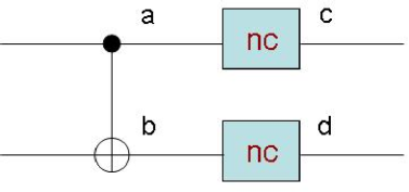
Figure 1: A possible scenario in a fault tolerant circuit.

In this case at locations $a,b$ we choose to apply the noisy operation $N^{Z}_{t}\otimes N^{Z}_{t}$ where $t$ is chosen so that the overall probability of any error at locations $a,b$ (of figure (1)) together, $t^{2}+2t(1-t)$, is equal to $p$, i.e.

$$p=t^{2}+2t(1-t)\Rightarrow t=1-\sqrt{1-p}.$$ (17)

Now the noise affecting each non-Clifford operation in circuit 1 is effectively independent. As in this section we assume the non-Clifford operations to be a phase rotation gate (a similar argument follows through for preparation of a phase state, with precisely the same numerical values), our goal is to work out when

$$(1-2p)(1-2(1-\sqrt{1-p}))=1-2q={1\over\sqrt{2}}$$ (18)

which has the solution for $p$ of:

$$p=10.41008383\%.$$ (19)

So under an adversarial EPG model, any circuit consisting of noisy Clifford operations and phase states and phase gates can have a fault tolerance threshold no higher than $10.41008383\%$.

IV Independent Depolarising thresholds for general non-Clifford unitaries

Depolarising noise commutes with all single qubit unitaries, so provided that the non-Clifford operations are single qubit unitaries the above reasoning applies straightforwardly. Although in this section we now allow $U$ to be any non-Clifford single qubit unitary, let us in particular take it to the most robust gate to depolarising noise, which in Buhrman is shown to be the $\pi/8$ phase gate anyway. Let us ask what $p$ is required such that (where as before time increases from left to right, $I$ denotes the identity operation, and $U$ represents the quantum operation acting by conjugation on density matrices, not just the unitary matrix itself)

$$U(\pi/4)(N^{D}_{p})^{2} = U(\pi/4)((1-p)I+pD)^{2}$$

$$= (1-p)^{2}U(\pi/4)+(1-(1-p)^{2})D$$

is a Clifford operation (the second line of this equation follows from the fact that $D^{2}=DU=UD=D$ as $D$ is the depolarising operation). We may now apply the bound obtained in Buhrman (a related result has been derived independently by Bravyi ) to give that the minimal such $p$ satisfies:

$$(1-p)^{2}=1-{6-2\sqrt{2}\over 7}=100\%-45.3\%$$ (20)

hence

$$p=1-\sqrt{1-{6-2\sqrt{2}\over 7}}=26.05\%$$ (21)

This upper bound applies regardless of the single qubit non-Clifford gates available and the fault tolerance methods used, provided that the basic gates are Clifford + single qubit unitaries.

Ben Reichardt Ben has independently previously performed a related analysis for simultaneous depolarising noise. The calculations are more difficult because in that case the noise does not commute straightforwardly. However, it is expected that an analysis of the simultaneous case would lead to upper bounds of a similar magnitude Ben .

V Specialising to Teleportation State-Injection schemes

If general bounds are required for architectures involving Clifford and non-Clifford operations, then it is generally not possible to shift more than two lots of noise onto each non-Clifford operation. This is because in principle every second operation in a given qubit wire could be a non-Clifford operation.

However, in many important proposals for fault tolerant quantum computation the non-Clifford operations are always surrounded by specific configurations of Clifford operations. This is because non-Clifford operations are often introduced into the computation using very specific ancilla preparation constructions. For example, one method that we will consider here is the technique of ‘state-injection’ - see figure (2). This method involves firstly creating a physical non-Clifford qubit, either by direct access to a source of such qubits, or by applying a gate such as the $\pi/8$ gate to a suitable Pauli-eigenstate. This qubit is then ‘teleported’ into an error correcting code, by first decoding one half of an encoded bell pair to the physical level (post-selecting on no errors), and then performing ordinary teleportation using CNOTs and X,Z measurements. Because the teleportation circuit immediately around the non-Clifford resource has around $5$ to $7$ non-trivial error locations (depending upon the precise model), one can shift upto $7$ lots of noise onto the non-Clifford resource, and obtain much lower upper bounds.

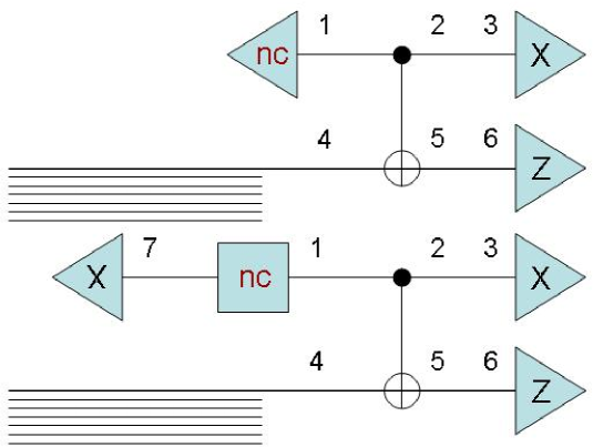
Figure 2: These circuits show two possible state injection settings. The boxes denote gates, the triangles are either preparation (of the +1 eigenstate) or measurement in the X,Z bases, and the collection of wires at the bottom left of each circuit represents the postselected decoding process. The letters ‘nc’ denote ‘non-Clifford’. The top circuit is for scenarios involving single qubit preparation as the non-Clifford resource, the second is for single qubit gates. Each diagram has locations numbered from 1 to 6, with the lower figure having an extra location 7. In the text we use these numbers to define noise models for both the upper and lower circuit in this figure. For state injection protocols these circuits represent the only way in which non-Clifford operations enter the computation.

By allowing noise at these locations, and then remodelling this as effective noise acting only upon the non-Clifford resource, it is possible to strengthen the bounds derived in the previous sections.

To illustrate the approach, let use consider what happens when in the top circuit of fig.(2) we apply various types of Pauli error at locations 2 to 6. The following arguments give some rules for ‘shifting’ these Pauli errors to location 1:

1. Application of $Z$ at location 6, and no errors elsewhere. Because location 6 is immediately followed by a $Z$ measurement, this case is essentially equivalent to no error as it is ‘absorbed’ by the measurement.

2. Application of $X$ at location 6, and no errors elsewhere. An $X$ on the target wire commutes with the CNOT, and so the $X$ can in fact be commuted through to location 4.

3. Application of Pauli error at location 4, and no errors elsewhere. Now because the CNOT and subsequent $X,Z$ measurements implement a Bell measurement, and because each projector $B$ onto a Bell state satisfies $(P\otimes I)B(P\otimes I)=(I\otimes P)B(I\otimes P)$ for any Pauli operation $P$, a Pauli $P$ at location 4 is equivalent to a $P$ acting at location 1. Putting this together with the previous point shows that an $X$ at location 6 is equivalent to an $X$ at location 1.

4. Application of $Y$ at location 6, and no errors elsewhere. A $Y$ error as a quantum operation (not as a matrix) is equivalent to a $Z$ error and an $X$ error. The $Z$ can be absorbed by the $Z$ measurement on the lower wire, leaving an $X$ error which can be moved to location 1 by the previous points. Hence a $Y$ at location 6 is equivalent to an $X$ at location 1.

5. Any Pauli errors at locations 4,5,6. Because Pauli matrices either commute or anticommute, when viewed as quantum operations Pauli errors actually commute with each other - consider for example the identity $XZ\rho ZX=ZX\rho XZ$. Hence the previous rules can be applied to any set of Pauli errors acting at locations 5,6 - effectively re-expressing them as Pauli errors acting with various probabilities at location 1.

6. Any Pauli errors at locations 2,3. Any $X$ errors can be absorbed by the $X$ measurement on the top wire, any $Z$ errors can be commuted through the CNOT to location 1.

We consider two variants of the state injection schemes. In state resource variants, the non-Clifford resource is a pure qubit state as in the top circuit of figure (2), in gate resource variant, the non-Clifford resource is a single qubit unitary, as in the bottom circuit of figure (2).

The above rules can be applied to any configuration of Pauli noise at locations $2$-$6$ to shift it all to location $1$, where it can attack the non-Clifford resource. As the non-Clifford resource at location $1$ is effectively a state in the Bloch sphere, we can solve the relatively simple problem of how much of this noise forces the state to enter the Clifford ‘octahedron’ (c.f. BK ; Ben magic ) formed from the convex hull of Pauli eigenstates. In the case of upper bounds for an EPG model, we are also free to try to pick the most adversarial noise we can. Consider a pure Bloch vector

$$\left(\begin{array}[]{c}x\\ y\\ z\end{array}\right)$$ (25)

in the positive octant of the Bloch sphere (i.e. $x,y,z\geq 0$). A $Z$ error flips the sign of $x,y$, an $X$ error flips the sign of $y,z$. Our goal is the find the minimal noise, for a given noise model, which takes the input Bloch vector to an output one

$${\rm Noise:}\left(\begin{array}[]{c}x\\ y\\ z\end{array}\right)\rightarrow\left(\begin{array}[]{c}x^{\prime}\\ y^{\prime}\\ z^{\prime}\end{array}\right)$$ (32)

satisfying $x^{\prime}+y^{\prime}+z^{\prime}=1$, which is the equation of the face of the octahedron in the positive octant (see e.g. figure (3)).

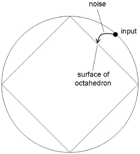
Figure 3: A 2D projection of the Bloch sphere. The goal of the calculations in this paper is to determine the noise strength required for an input state to enter the octahedron formed from the convex hull of the Pauli eigenstates.

VI Bounds for the Knill noise model and teleportation state-injection, for phase state and phase gate resources.

To be perfectly clear, it is important to specify precisely how we apply Knill’s noise model to the circuits in figure 2. In the top circuit of figure 2 we apply: a $Z$ at locations 1,3 with probability $4\gamma/15$; an $X$ at location 6 with probability $4\gamma/15$; and at locations 2,5 considered together we apply each of the 15 non-identity pairs of operators chosen from $I,X,Y,Z$, each pair with probability $\gamma/15$. Note that we have kept location 4 error free. The noise at location 4 will be determined by the decoding circuit that feeds it, and so in order to obtain general bounds independent of the codes used we are adopting a noise model that is strictly weaker than Knill’s. Later we will discuss the effect that noise in the decoding circuits might have.

In the bottom circuit of figure 2, on the other hand, we apply the noise model: at 3,7 we apply a $Z$ with probability $4\gamma/15$; at 6 an $X$ with probability $4\gamma/15$; at 1 we apply a $X,Y$ and $Z$ each with probability $4\gamma/15$; and at locations 2,5 considered together each of the 15 non-identity pairs of operators chosen from $I,X,Y,Z$, each pair with probability $\gamma/15$. Again we keep location 4 error free.

Using this noise model leads to the following effective transformation of the input Bloch vector:

$$\left(\begin{array}[]{c}x^{\prime}\\ y^{\prime}\\ z^{\prime}\end{array}\right)=\left(1-{16\gamma\over 15}\right)^{n}\left(1-{8\gamma\over 15}\right)\left(\begin{array}[]{c}(1-8\gamma/15)x\\ (1-8\gamma/15)^{2}y\\ (1-8\gamma/15)z\end{array}\right)$$ (39)

where $n=1$ for the top circuit of figure (2), and $n=2$ for the lower circuit of figure (2). Our goal is hence to determine, for a given input resource, the minimal $\gamma$ such that the output Bloch vector lies on the face of the octahedron.

For example, if we assume that the ideal state entering location 1 in both circuits is $|\pi/4\rangle$, either because that is the state prepared, or because the non-Clifford unitary is the $\pi/8$ gate, then find the solution:

$$(1-16\gamma/15)(1-8\gamma/15)^{2}(1+(1-8\gamma/15))=\sqrt{2}$$

$$\Rightarrow \gamma\sim 13.6861\%.$$ (40)

for the top circuit of figure 2, and

$$(1-16\gamma/15)^{2}(1-8\gamma/15)^{2}(1+(1-8\gamma/15))=\sqrt{2}$$

$$\Rightarrow \gamma\sim 9.5858\%.$$ (41)

for the lower circuit of figure 2. Similar equations can be derived and solved for any possible phase gate and phase state resource. It is not difficult to solve for the minimal $\gamma$ that leads to an output vector on the face of the octahedron. Numerically scanning through these solutions suggests that the $|\pi/4\rangle$ and $U(\pi/4)$ resources are not actually the most robust non-Clifford phase state or phase gate resources in this setting, although they are very close. If we allow all phase state and phase gate resources respectively, the upper bounds become:

$$\gamma\sim 13.71\%$$ (42)

for phase states, and

$$\gamma\sim 9.59\%$$ (43)

for phase gates. Later we present the values obtained if any single qubit state or gate is permitted as the non-Clifford resource.

VII Bounds for an EPG noise model and for phase gate or phase state teleportation state injection

To obtain upper bounds for an adversarial EPG model, we will pick noise which appears as detrimental as possible, yet is sufficiently simple to analyse. It is quite likely that the noise that we pick at each location is not the most adversarial (in the sense of pulling the teleportation circuit into a Clifford operation) within the EPG constraint, but this would require further analysis.

We choose the following noise for the top circuit of figure (2). Assume that the input non-Clifford state is $|\theta\rangle$. Apply $O^{|\theta\rangle\langle\theta|}_{p}$ at location $1$; $N^{Z}_{p}$ at locations 3,4; $N^{X}_{p}$ at location $6$; and replace the CNOT with $O^{|\theta\rangle\langle\theta|}_{p}$ (see eq. (6)) on the top wire followed by a CNOT. This gives the following transformation on the input Bloch vector (which has $z=0$ as it is a phase state):

$$\left(\begin{array}[]{c}x\\ y\end{array}\right)\rightarrow(1-2p)^{2}((1-p)(1-2p)-p)\left(\begin{array}[]{c}x\\ (1-2p)y\end{array}\right).$$ (48)

For an input state $|\theta=\pi/4\rangle$, the minimal $p$ such that the output Bloch vector lies on the face of the octahedron is:

$$p=3.68124\%.$$ (49)

Numerics again suggest that $|\theta=\pi/4\rangle$ is not the most robust state in this setting, and in fact

$$p=3.69\%$$ (50)

is a noise level sufficient to take all possible phase states into the octahedron.

For the lower circuit of figure (2) we choose the following noise. Assume that the input state is $|+\rangle$, the $+1$ eigenstate of $X$, and that $U$ is the non-Clifford phase gate. Apply $O^{|+\rangle\langle+|}_{p}$ at location $7$; $O^{U|+\rangle\langle+|U^{{\dagger}}}_{p}$ at location $1$; $N^{Z}_{p}$ at locations $3$,$4$; $N^{X}_{p}$ at location $6$; and replace the CNOT with $O^{U|+\rangle\langle+|U^{{\dagger}}}_{p}$ on the top wire followed by a CNOT. This gives the following transformation on the output Bloch vector (which has $z=0$ as it is a phase state):

$$(1-2p)^{2}((1-p)(1-4p+2p^{2})-p)\left(\begin{array}[]{c}x\\ (1-2p)y\end{array}\right).$$ (53)

For an input state $U(\theta=\pi/4)$ the minimal $p$ such that the output Bloch vector lies on the face of the octahedron is:

$$p=3.00339\%.$$ (54)

Numerics suggest that $U(\theta=\pi/4)$ is not the most robust phase gate in this setting, and in fact

$$p=3.01\%$$ (55)

is a noise level sufficient to take all possible phase states into the octahedron.

VIII Bounds for teleportation injection with general Non-Clifford states and gates

It is not difficult to perform the analysis of the previous two sections using general single qubit non-Clifford gate and state resources, and then to numerically calculate the most robust of these resources. For the Knill noise model we find that for general unitary gates

$$\gamma=15.19\%$$ (56)

is sufficient to turn the teleportation state-injection into a Clifford circuit, whereas for general states

$$\gamma=21.78\%$$ (57)

is sufficient. The most robust non-Clifford state entering the circuit appears to be close to, but not exactly the same as, the so-called $|T\rangle$ state.

For an EPG model we use the same noise as for the phase gates/states in the previous section, except at location $4$ instead of applying $N^{Z}_{p}$ we apply $N^{Y}_{p}$. Numerical analysis of the resulting equations finds that:

$$p=5.03\%$$ (58)

is sufficient to turn the teleportation state-injection into a Clifford circuit, whereas for general states

$$p=6.31\%$$ (59)

is sufficient.

IX Potential effects of the decoding circuits.

So far, we have considered solely the injection part of the circuit as depicted in fig. 2, and have not attempted to understand the effects of noise in the decoding circuit. Indeed, within the framework of Knill’s noise model we have not even allowed noise at location 4. The precise form of the noise generated by the decoding circuit is difficult to determine due to the complex structure of the encoding and decoding networks, which may include many steps of concatenation. This brings with it two problems. Firstly, the entangling gates in the decoder typically generate correlations in noise which mean that the problem becomes a multiqubit problem, rather than a simple geometrical problem on one or two qubits. Secondly, the postselection steps have an effect on the noise profile, and this is difficult to calculate.

However, we believe that a careful analysis of the decoding circuits will lead to improvements in the bounds that we have presented. In this section we present some very rough indications of the level of improvement that might be expected, although a more careful analysis is left to another occasion.

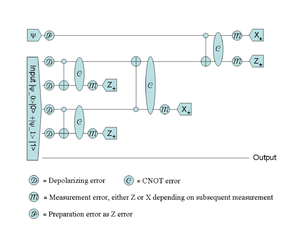
Figure 4: This circuit shows the state-injection circuit of fig. 2 (lines 1 and 2) but now we explicitly include the action of part of a decoding circuit with the Knill error model. The input of the circuit is the state $(|\psi_{0}\rangle|0\rangle+|\psi_{1}\rangle|1\rangle)/\sqrt{2}$ where the state $|\psi_{i}\rangle$ will be decoded by an error free circuit to $|i\rangle$ in the second qubit. Errors from previous stages of encoding and manipulation are modelled by depolarizing errors. The error free state-injection would then lead to the preparation of the state $|\psi\rangle$ in the Output qubit at the bottom. Determining the minimal error rate that ensures that the Output is a stabilizer state provides an upper bound on the fault tolerance threshold.

To get a feeling for the effect of the errors that are introduced by the decoding circuit that immediately precedes position $4$ we have carried out an analysis of the circuit in fig. 4, which corresponds to one level of decoding prior to the injection circuit for a particular code. The input of the top arm of the teleporter is a phase state proportional to $|0\rangle+\exp(i\pi/4)|1\rangle$. This circuit is a simplified version of Fig. 9 of 0402171 . The simplification consists of neglecting essentially all errors that may occur in the preparation and encoding, as well as the decoding of the lower half of that circuit of Fig. 9 of 0402171 . We also model the error on the incoming qubits in fig. 4 via depolarizing errors (it is in this assumption that most of the complexity is buried).

The computation of the error threshold in this approach is possible analytically because of the small circuit size. With the help of a computational mathematical package we find the threshold to be the sole real root of the polynomial

$$p(e_{c})=-\frac{1}{2}-\frac{f_{1}(e_{c})}{f_{2}(e_{c})}$$

with

$$f_{1}(e_{c}) = (16e_{c}-15)^{5}(225-180e_{c}+32e_{c}^{2})^{2}\times$$

$$\times (16875-40500e_{c}+46800e_{c}^{2}-23040e_{c}^{3}+4096e_{c}^{4})$$

$$f_{2}(e_{c}) = 1125\sqrt{2}(576650390625-3536789062500e_{c}$$

$$+ 11768793750000e_{c}^{2}-24002325000000e_{c}^{3}$$

$$+ 32367600000000e_{c}^{4}-29499033600000e_{c}^{5}$$

$$+ 18141511680000e_{c}^{6}-7375159296000e_{c}^{7}$$

$$+ 1887436800000e_{c}^{8}-273804165120e_{c}^{9}$$

$$+ 17179869184e_{c}^{10})$$

and we find

$$e_{c}^{threshold}=9.2888\%$$ (60)

One can try to understand how critical is the choice of depolarising errors entering the decoding steps. To estimate this we also analysed what happens if the depolarising errors in the central four wires of figure (4) are removed. In this case the bound becomes

$$e_{c}^{threshold}=10.0638\%$$ (61)

Both these bounds are quite close to the bound that would be obtained by instead modelling the noise from the decoding circuit as a depolarising error at location 4 (for which the bound would be 9.59%). All these numbers should be compared to 13.69%, which is the number obtained for precisely the same phase state input with no noise whatsoever outside locations 1-3 and 5-7 of Fig. 2.

A more rigorous analysis of the decoding circuits requires much more effort and may be reported elsewhere. However, these rough calculations give some indication of the improvements that might be expected in the upper bounds that we have obtained so far.

Table 1: A summary of upper bounds presented in this work. ‘Injection’ refers to teleportation state-injection. ‘NC’ means non-Clifford.

NC resources	Method	Noise Model	Upper bound
phase gates/states	any	independent $N^{Z}_{p}$	7.96 %
phase gates/states	any	EPG	10.41%
all gates	any	indep. depolarizing	26.05%
phase gates	injection	Knill	9.59%
phase states	injection	Knill	13.71%
phase gates	injection	EPG	3.01%
phase states	injection	EPG	3.69%
all gates	injection	Knill	15.19%
all states	injection	Knill	21.78%
all gates	injection	EPG	5.03%
all states	injection	EPG	6.31%

X Discussion, Caveats, and Conclusion

We have discussed ‘attacks’ on fault tolerant quantum circuits involving Clifford operations and extra resources, with the intention of adding the smallest amount of noise possible to make the circuits efficiently simulatable classically. The approach is simple - to shift noise from neighbouring Clifford gates onto the non-Clifford resources. The approach works best for situations where this ‘shifting’ process can be done easily, as happens for teleportation based state injection schemes. There are many other fault tolerance proposals in the literature (e.g. methods built around cluster states Cluster ) that involve a few non-Clifford resources surrounded by many Clifford operations - and so in such cases our approach could also provide improved upper bounds, depending upon the precise manner in which the ‘non-Cliffordness’ is ‘injected’ into the rest of the circuit.

We are certain that the upper bounds obtained in this work can be optimised further, particularly through consideration of the decoding circuits. The rigorous part of the analysis performed in this work does not consider the decoding circuit present in state-injection schemes, except for a noise step at location 4 in the error-per-gate noise model. The analysis of the teleportation part of the state-injection is straightforward because the teleportation circuit simplifies correlated Pauli errors, reducing the problem to a single-qubit one. A more sophisticated attack that also applies noise to the decoding steps should lead to tighter bounds, especially for Knill’s noise model.

It is also important to note that teleportation is not the only method of state injection. If the non-Clifford resource is either a measurement or a unitary, a non-Clifford measurement may be implemented directly on the decoded wire. This method involves far fewer error locations outside the decoder, and hence is less susceptible to our method of attack. Hence the bounds derived in the lower part of table (1) are not generally applicable to all stabilizer schemes, but are intended more as an approach that can be fairly effective for specific fault tolerance proposals.

A summary of the upper bounds that we have obtained is given in table (1). Although the bounds that we have derived are lower than previous rigorously established upper bounds, our bounds are not typically as general as most previous results make fewer assumptions about the architecture (and often involve incomparable noise models). For comparable fault tolerance schemes the estimates conjectured in [7] are lower than the values that we have obtained, and future work will be needed to see whether further optimisation of our approach will go as low. However, the approach presented here is relatively simple, makes no assumptions (other than assuming that quantum computation is not classically tractable), and has a slightly different aim as it deals with ‘classical’ bounds rather than ‘quantum’ ones.

XI Acknowledgements

We thank EU-STREP CORNER, the EU Integrated Project QAP, the EPSRC QIP-IRC and the Royal Society for financial support. We are grateful to Ben Reichardt for discussions and for valuable comments on an earlier draft.

References

- (1) E. Knill, Nature, 434, 39, (2005).
- (2) see e.g. A. Steane, Phys. Rev. A, 68, 042322 (2003). D. Aharonov & M. Ben-Or, Proc. 29th ACM STOC, p.176 (1997), quant-ph/9906129; A. Kitaev, Russ. Math. Surveys, 52, 1191 (1997); D. Gottesman, Phys. Rev. A, 57 127 (1998); B. Reichardt, PhD thesis, arXiv:quant-ph/0612004; P. Aliferis, PhD thesis, arXiv:quant-ph/0703230.
- (3) A. Harrow and M. Nielsen, Phys. Rev. A 68, 012308 (2003) (quant-ph/0301108)
- (4) S. Virmani, S. F. Huelga, and M. B. Plenio, Phys. Rev. A, 71, 042328 (2005).
- (5) H. Buhrman, R. Cleve, M.Laurent, N. Linden, A. Schrijver and F. Unger, Proc. 47 Symp. FOCS (2006)
- (6) J. Kempe, O. Regev, F. Unger, and R. de Wolf, arXiv:0802.1464
- (7) J. Fern, arXiv:0801.2608
- (8) S. Bravyi, private communication, (2005).
- (9) S. Bravyi and A. Kitaev, Phys. Rev. A 71, 022316, (2005).
- (10) D. Aharonov, M. Ben-Or, R. Impagliazzo, N. Nisan, arXiv:quant-ph/9611028;
- (11) A. A. Razborov, Quant. Inf. Comp., 4 222-228 (2004) (quant-ph/0310136)
- (12) A. Kay, Phys. Rev. A 77, 052319 (2008).
- (13) M. A. Nielsen and I. L. Chuang, ‘Quantum Information and Computation’, CUP (2000).
- (14) D. Gottesman, PhD thesis, quant-ph/9705052
- (15) R. Jozsa and N. Linden, Proc. Roy. Soc. A 459, 2011 (2003).
- (16) P. Aliferis, D. Gottesman, and J. Preskill, Quant. Inf. Comp., 8 181-244 (2008) (quant-ph/0703264).
- (17) B. Reichardt, FOCS 2006, arXiv:quant-ph/0608018 (2006).
- (18) B. Reichardt, Quant. Inf. Proc., 4, 251, (2005).
- (19) Ben Reichardt, private communication, (2008).
- (20) E. Knill, arXiv:quant-ph/0402171v1.
- (21) R. Raussendorf and H. J. Briegel, Phys. Rev. Lett., 86, 5188 (2001).