Finding SDSS BALQSOs Using Non-Negative Matrix Factorisation

Abstract

Modern spectroscopic databases provide a wealth of information about the physical processes and environments associated with astrophysical populations. Techniques such as blind source separation (BSS), in which sets of spectra are decomposed into a number of components, offer the prospect of identifying the signatures of the underlying physical emission processes. Principle Component Analysis (PCA) has been applied with some success but is severely limited by the inherent orthogonality restriction that the components must satisfy.

Non-negative matrix factorisation (NMF) is a relatively new BSS technique that incorporates a non-negativity constraint on its components. In this respect, the resulting components may more closely reflect the physical emission signatures than is the case using PCA. We discuss some of the considerations that must be made when applying NMF and, through its application to the quasar spectra in the Sloan Digital Sky Survey (SDSS) DR6, we show that NMF is a fast method for generating compact and accurate reconstructions of the spectra.

The ability to reconstruct spectra accurately has numerous astrophysical applications. Combined with improved SDSS redshifts, we apply NMF to the problem of defining robust continua for quasars that exhibit strong broad absorption line (BAL) systems. The resulting catalogue of SDSS DR6 BAL quasars will be the largest available. Importantly, the NMF approach allows quantitative error estimates to be derived for the Balnicity Indices as a function of key astrophysical and observational parameters, such as the quasar redshifts and the signal-to-noise ratio of the spectra.

1 Introduction

The scale of modern spectroscopic surveys such as the Sloan Digital Sky Survey (SDSS) demand the development and application of new analysis techniques that are able to condense the vast quantities of available data to extract useful results. Blind source separation (BSS) techniques are a family of techniques that enable such a condensation of information. A BSS technique can take a set of spectra written as a matrix, $V$, and generate a corresponding set of components, $H$, that can be linearly combined to recreate the original data using a set of weighting coefficients, $W$:

$$V=WH.$$ (1)

The form of the components depends on the particular technique used.

The most widely used BSS technique in astronomy is principal component analysis (PCA), which generates orthogonal components. PCA has been successfully applied for a number of purposes but interpretation of the component spectra is limited by their orthogonality. In this work we describe non-negative matrix factorisation, a recently-developed BSS technique, and demonstrate its application to the reconstruction of absorbed quasar continua in the SDSS.

2 Non-Negative Matrix Factorisation

2.1 Definition

Non-negative matrix factorisation (NMF) is a relatively new BSS technique that incorporates a non-negativity constraint on both its components and their weights Lee and Seung (1999, 2000); Blanton and Roweis (2007). The non-negativity constraint is appealing in the context of spectroscopic data as the physical emission signatures are expected to naturally obey this restriction. Unusually for a BSS technique, fewer components are generated than there are input spectra. Starting from random initial matrices, the components ($H$) and weights ($W$) follow the multiplicative update rules

$$W_{ik}\leftarrow W_{ik}\frac{[VH^{T}]_{ik}}{[WHH^{T}]_{ik}},$$ (2)

and

$$H_{kj}\leftarrow H_{kj}\frac{[W^{T}V]_{kj}}{[W^{T}WH]_{kj}}.$$ (3)

As fewer components are generated than there are input spectra the reconstructions $WH$ will in general be approximations to the data; the update rules minimise the error in the approximations, as measured by the Euclidean distance between the reconstructions and the data. The random starting conditions result in slightly different components being generated each time the algorithm is executed, but the resulting reconstructions do not vary.

When components and weights have been generated from one set of input spectra, the components can be applied to generate reconstructions of other spectra. In this case random initial weights are used, which are updated according to equation 2, while the components are held fixed.

2.2 Practicalities of Applying NMF

2.2.1 Number of Components

In applying NMF to any dataset the number of components must be pre–specified. Increasing the number of components will always increase the precision of the reconstructions, but the increased precision is not always desirable. With too many components it becomes beneficial for the NMF procedure, in terms of the total error in the reconstructions, to overfit a small number of particularly noisy or very unusual spectra, incorporating their noise, or their unique features, in the components. It is thus most effective to employ the maximum number of components that does not produce overfitting in any subset of spectra. The optimal number of components must be chosen separately for each sample. For reconstructions of the SDSS quasar spectra the number is between 8 and 15, with the appropriate number determined via a simple trial and error scheme.

2.2.2 Sample Selection

Some care must be taken when selecting the sample to use as inputs to the NMF algorithm. A larger sample will better constrain the resulting components, but this must be balanced against the increased CPU time required for the calculations. A sample size of around 500 has been found to produce well-constrained components while completing in a reasonable time on a modern desktop computer.

The range of properties of the sample spectra should reflect the range of properties of the population from which they are drawn. Individual objects with very unusual properties can cause problems by inducing overfitting at a smaller number of components than would otherwise be the case. In such cases the most extreme objects must be removed from the sample.

2.2.3 Redshifts

Before a source separation can be performed the input spectra must be shifted to their respective rest frames. Accurate redshifts are required to ensure that specific features occur in the same location in all spectra. Redshift errors of $\sim 0.001$ are sufficient to blur narrow features when viewed across the sample, reducing the quality of the NMF reconstructions.

In the following work the redshifts used were recalculated from the SDSS spectra in order to reduce the errors and biases present in the SDSS redshifts, which are each as large as $\pm 0.005$ at redshifts $z>2$. At low redshifts the new values were calculated from the positions of the [O iii] and [O ii] emission lines, while at higher redshifts improved cross-correlation measures were developed that are unbiased with respect to the narrow emission line redshifts at low-redshift.

2.2.4 Dust Reddening

NMF reconstructs the observed spectra as a linear combination of components, assuming all contributions are additive. In contrast, dust reddening multiplies the spectra by a wavelength-dependent flux ratio. For moderate levels of reddening this effect is smaller than the natural object-to-object variations between spectra and is accounted for in the NMF components, but this is not the case for the most heavily obscured objects.

To improve the quality of the reconstructions of heavily reddened objects an estimate of the unreddened spectrum can be made. By multiplying the observed spectrum by a power law slope it can be given a slope within the typical range for the object being observed. The edited spectrum is then used as an input for the NMF algorithm, and the results can be divided by the same power law slope to match the observed spectrum.

3 Application to Broad Absorption Line Quasars

3.1 Broad Absorption Line Quasars

Broad absorption line quasars (BALQSOs) are quasars that exhibit strong broad absorption line (BAL) systems, with velocity widths often in excess of 10 000 km s^-1. They are always intrinsic to the quasar, although they may be blueshifted with respect to the active galactic nucleus (AGN) by over 20 000 km s^-1. The blueshift is taken to mean that the BAL systems are part of large-scale outflows driven by the AGN.

Methods of classifying BALQSOs vary, but the most widely used measure is the balnicity index (BI) Weymann et al. (1991), defined as

$${\rm BI}=-\int_{25000{\rm\ km\ s}^{-1}}^{3000{\rm\ km\ s}^{-1}}\left(1-\frac{f(v)}{0.9}\right)C{\rm d}v,$$ (4)

where $f(v)$ is the continuum-normalised flux as a function of velocity, $v$, relative to the line centre. The constant $C$ is equal to 1 in regions where $f(v)$ has been continuously less than 0.9 for at least 2000 km s^-1, and 0 elsewhere.

Depending on the measure used, the observed BAL fraction is between 10 and 15 per cent Weymann et al. (1991); Trump et al. (2006); Knigge et al. (2008); the fraction increases to 17 to 22 per cent when corrected for differential selection effects between BAL and non-BAL quasars. The presence of BAL systems in some, but not all, quasars could be the result of an orientation effect Weymann et al. (1991); Schmidt and Hines (1999), or BALQSOs could represent a particular stage in the quasar life-cycle Voit et al. (1993); Becker et al. (2000).

3.2 Application of NMF

In order to characterise BALQSOs, estimates of the unabsorbed continua are required, which we have generated using the NMF technique. Samples of spectra, each consisting of 500 non-BAL quasars, was selected to cover all redshifts, $0.7<z<2.6$, in redshift bins of width $\Delta z=0.1$. The NMF algorithm was applied to each sample to produce NMF component spectra, applicable to quasars within a specified redshift interval.

The resulting components were used to reconstruct the continua of potential BALQSO spectra. During this fitting the components were held fixed and only the weights were updated, following equation 2. All regions where broad absorption is likely to occur were initially masked, and the mask was then iteratively updated by comparing the resulting reconstructed continuum with the observed spectrum. The NMF fitting was recalculated after each mask update; in most cases the mask locations reached a stable solution after only two or three iterations.

The classification of quasars into BAL and non-BAL categories is sensitive to the redshift used in the calculations, as an inaccurate redshift can move absorption features into or out of the velocity range examined. An inaccurate redshift will also reduce the quality of any estimate of the continuum. Unfortunately, inaccurate redshifts are more likely for BALQSOs, as the absorption of the blue wing of the C iv line means that any method using this line will overestimate the redshift. The redshift measurements used here do not normally use the regions of the spectra that exhibit broad absorption, so they are not expected to be significantly affected by this bias.

At redshifts $z\geq 2.6$ there are insufficient non-BAL quasars with adequate signal-to-noise ratio (SNR) available to produce useful components. However, due to the Ly$\alpha$ forest, no additional quasar “continuum” enters the spectra at these redshifts so the components from the $2.5\leq z<2.6$ redshift bin were used to fit quasars with $z\geq 2.6$.

3.3 Results

The NMF-procedure described above has been applied to generate estimated continua for over 80 000 quasar spectra with redshifts $0.7<z<4.4$. Example reconstructions of BALQSO continua with a range of redshifts and BI values are shown in Figure 1.

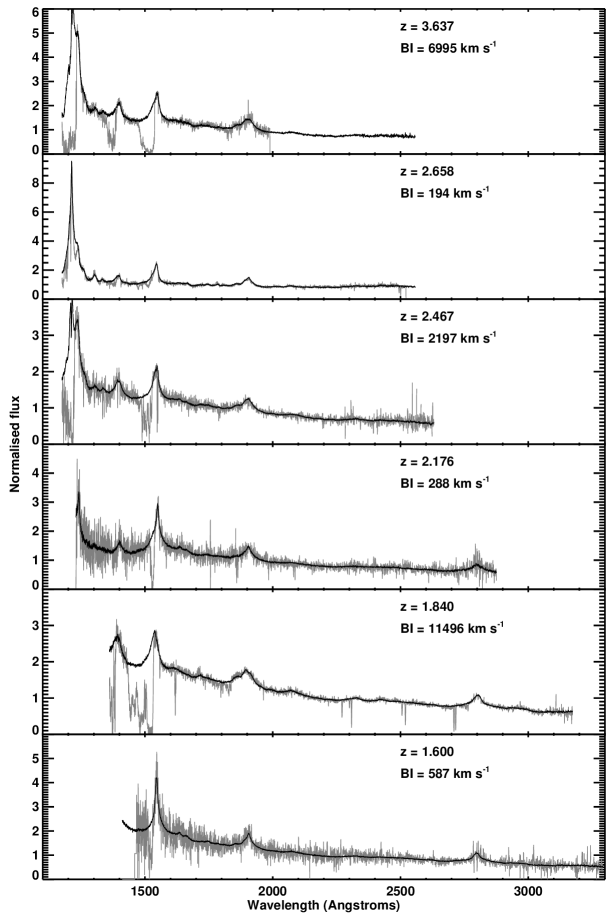
Figure 1: Example reconstructions (black curves) of BALQSO continua, based on their observed spectra (grey curves). Redshifts and balnicity indices are as shown in the panels.

In order to quantify the accuracy with which the continua are reconstructed, a set of synthetic BALQSO spectra were created. First, continua were fitted to a set of 105 BALQSOs, redshifts $2.25<z<2.35$, with high SNR spectra, using the procedure outlined above. A flux-ratio spectrum for each BALQSO was generated by dividing the observed spectrum by the reconstruction, then smoothing to remove noise. A set of randomly chosen, non-BAL quasar spectra were then multiplied by the flux ratio spectra, generating synthetic BALQSO spectra for which the unabsorbed continua were known.

Continua were fitted to the synthetic BALQSO spectra by the same method as for genuine BALQSOs, and the resulting BI measurements were compared to the real BI values of the input flux ratios as a quantitative test of the NMF procedure. The results are shown in Figure 2 (a). In most cases there is good agreement between the input and measured values, but the BI is frequently undermeasured. The undermeasurement is due largely to the effect of noise in the lower SNR spectra: a single pixel with positive noise that brings its value above 90% of the continuum can prevent a large velocity interval from contributing to the BI measurement.

Figure 2: (a) Measured BI values for a set of synthetic BALQSO spectra with known input BI. (b) As (a) but with the flux ratios smoothed before the BI is measured.

Figure 2 (b) shows the BI values measured when the noise is reduced by smoothing the measured flux ratios in the same way as for the input flux ratios. The smoothing reduces significantly the number of systems in which the BI is undermeasured, resulting in an RMS residual of 250 km s^-1 with a mean offset of only 20 km s^-1.

The effect of noise in BI calculations has been noted previously Knigge et al. (2008) but to date it has not been quantified. A forthcoming analysis of the undermeasurement of the BI at different signal-to-noise ratios will allow an accurate determination of the BAL fraction as a function of quasar luminosity and redshift.

4 Conclusions

Non-negative matrix factorisation shows much promise as a technique for analysis of modern spectroscopic surveys such as the SDSS. We have demonstrated here its application to the problem of estimating the continua of BALQSOs. Component spectra were generated from sets of non-BAL quasars, and then used in conjunction with iteratively defined masks to identify regions of absorption in other quasar spectra and reconstruct their continua.

The effectiveness of the NMF continuum definition has been demonstrated using simulated BALQSO spectra. The BI values of BALQSOs are often undermeasured due to the influence of limited signal-to-noise ratio in the observed spectra. A forthcoming analysis of this undermeasurement effect will allow the BAL fraction in the SDSS spectroscopic survey to be quantified as a function of key parameters such as quasar redshift and luminosity.

References

- Lee and Seung (1999) D. D. Lee, and H. S. Seung, Nature 401, 788–791 (1999).
- Lee and Seung (2000) D. D. Lee, and H. S. Seung, Adv. Neural Inf. Processing Syst. 13, 556–562 (2000).
- Blanton and Roweis (2007) M. R. Blanton, and S. Roweis, AJ 133, 734–754 (2007).
- Weymann et al. (1991) R. J. Weymann, S. L. Morris, C. B. Foltz, and P. C. Hewett, ApJ 373, 23–53 (1991).
- Trump et al. (2006) J. R. Trump, P. B. Hall, T. A. Reichard, G. T. Richards, D. P. Schneider, D. E. Vanden Berk, G. R. Knapp, S. F. Anderson, X. Fan, J. Brinkman, S. J. Kleinman, and A. Nitta, ApJS 165, 1–18 (2006).
- Knigge et al. (2008) C. Knigge, S. Scaringi, M. R. Goad, and C. E. Cottis, MNRAS 386, 1426–1435 (2008).
- Schmidt and Hines (1999) G. D. Schmidt, and D. C. Hines, ApJ 512, 125–135 (1999).
- Voit et al. (1993) G. M. Voit, R. J. Weymann, and K. T. Korista, ApJ 413, 95–109 (1993).
- Becker et al. (2000) R. H. Becker, R. L. White, M. D. Gregg, M. S. Brotherton, S. A. Laurent-Muehleisen, and N. Arav, ApJ 538, 72–82 (2000).