Standing on the shoulders of giants

Abstract

Context. Centimeter and meter-sized solid particles in protoplanetary disks are trapped within long-lived, high-pressure regions, creating opportunities for collapse into planetesimals and planetary embryos.

Aims. We aim to study the effect of the high-pressure regions generated in the gaseous disks by a giant planet perturber. These regions consist of gas retained in tadpole orbits around the stable Lagrangian points as a gap is carved, and the Rossby vortices launched at the edges of the gap.

Methods. We performed global simulations of the dynamics of gas and solids in a low mass non-magnetized self-gravitating thin protoplanetary disk. We employed the Pencil code to solve the Eulerian hydro equations, tracing the solids with a large number of Lagrangian particles, usually 100 000. To compute the gravitational potential of the swarm of solids, we solved the Poisson equation using particle-mesh methods with multiple fast Fourier transforms.

Results. Huge particle concentrations are seen in the Lagrangian points of the giant planet, as well as in the vortices they induce at the edges of the carved gaps. For 1 cm to 10 cm radii, gravitational collapse occurs in the Lagrangian points in less than 200 orbits. For 5 cm particles, a 2 $M_{\oplus}$ planet is formed. For 10 cm, the final maximum collapsed mass is around 3 $M_{\oplus}$. The collapse of the 1 cm particles is indirect, following the timescale of gas depletion from the tadpole orbits. Vortices are excited at the edges of the gap, primarily trapping particles of 30 cm radii. The rocky planet that is formed is as massive as 17 $M_{\oplus}$, constituting a Super-Earth. Collapse does not occur for 40 cm onwards. By using multiple particle species, we find that gas drag modifies the streamlines in the tadpole region around the classical L4 and L5 points. As a result, particles of different radii have their stable points shifted to different locations. Collapse therefore takes longer and produces planets of lower mass. Three super-Earths are formed in the vortices, the most massive having 4.5 $M_{\oplus}$.

Conclusions. A Jupiter-mass planet can induce the formation of other planetary embryos at the outer edge of its gas gap. Trojan Earth-mass planets are readily formed; although not existing in the solar system, might be common in the exoplanetary zoo.

1 Introduction

Losing angular momentum by friction with the ambient gaseous headwind, centimeter to meter-sized bodies in protoplanetary disks spiral into the star on timescales as short as a hundred years (Weidenschilling 1977). Avoiding this fate is a major unsolved problem in modern astrophysics. The question of the formation of rocky planets is intimately connected with this problem, since the kilometer-sized bodies (planetesimals) whence they are believed to form (Safronov 1969) must be formed faster than the already rapid timescale of radial drift of the rocks (0.1-1 meter-size) and boulders (1-10 meter-size).

As colliding boulders have very poor sticking properties (Benz 2000), a possible scenario for the formation of planetesimals is direct gravitational collapse of the layer of boulders (Goldreich & Ward 1973). This hypothesis has met with criticism because no route for achieving critical densities could be found (Weidenschilling & Cuzzi 1993), but it has recently gained momentum due to a series of advances in modeling the coupled dynamics of gas and boulders through both analytical calculations and numerical simulations. Youdin & Goodman (2005) showed that when rocks and boulders migrate due to the drag force, they trigger a streaming instability that develops into a traffic jam in their migrating flow, with dramatic effects for the particle concentrations (Johansen et al. 2006b, Paardekooper 2006, Johansen & Youdin 2007, Balsara et al. 2008). Fromang & Nelson (2005) modeled the dynamics of particles in magnetized global disks and showed that trapping occurs in the pressure maxima of the turbulence generated by the magneto-rotational instability (MRI). The number of particles, however, was too low ($\leq$ 3000) to say anything about possible gravitational collapse. Johansen et al. (2006a) simulated the flow in an MRI-active local box using a statistically significant number of particles ($10^{6}$), and showed that the particle concentration is high enough to achieve critical densities.

Studies with self gravity to follow the collapse are restricted to local boxes (Johansen et al. 2007) and the massive disk case (Rice et al. 2004, Rice et al. 2006). The former couples the effects of particle concentrations due to the streaming instabilities with those due to the turbulence generated by the MRI to show that the turbulent layer of boulders locally collapse into dwarf planets on very short timescales. The latter is a global disk calculation of marginally gravitationally unstable gaseous disks, where boulders are shown to concentrate in the spiral arms that develop, where they also achieve critical density.

A broad conclusion that can be drawn from these studies is that any region with higher pressure than its surroundings tends to concentrate solids (Haghighipour & Boss 2003). Therefore, in order to trigger collapse of the solids, one has to create long-lived, high-pressure regions in the gas phase. A perturber, then, is expected to have major consequences in the dynamics of embedded rocks and boulders. Paardekooper & Mellema (2004) studied the dynamics of dust in a gaseous disk, finding that even low mass planets carve a deep dust gap. An update by Paardekooper (2007) showed an interesting feature. As early as 20 orbits, meter-sized particles tend to concentrate at the gap edges and at co-rotation in tadpole orbits. However, as Lagrangian trapping was not the main scope of their study, they did not further assess the consequences of particle concentration in 1:1 resonance, focusing instead on the other mean motion resonances brought about by the planet.

Fouchet et al. (2007) also explored the same problem, in 3D SPH simulations, considering not only different particle radii, but also different masses for the perturber. The results are very similar to those of Paardekooper (2007), but they argue against the accumulation they see being the result of resonance trapping. They come to this conclusion because the signatures of resonance trapping, easily identifiable in a eccentricity vs. semi-major axis plot for decoupled particles, disappears when one considers gas drag. Instead, they claim that it occurs more likely due to the dust concentrating at the gas pressure maxima at the edges of the gap. Fouchet et al. (2007) also notice that the 1 m sized boulders are found in 1:1 resonance at later times. They speculate that the same occurs for other particle sizes they considered (10 cm and 1 cm sized pebbles), but as the dust gap in this case was too narrow compared to the extended disk they considered (20 AU), they could not spot the rocks trapped in the co-orbital region.

One possibility that was unexplored in these works is whether a direct collapse can occur at the enhanced particle concentrations. There are significant gas overdensities in co-rotation, especially at the Lagrangian points, for at least 200 orbits (de Val-Borro et al. 2006). In these regions, the solids are subject to drag forces for a period long enough to allow concentration and eventual collapse into kilometer-sized bodies in 1:1 resonance. In this paper, we show that the trapping provided in the Lagrangian points is so efficient that the final mass of the collapsed body is that of terrestrial planets.

The collapse of the solids that get trapped at the edges of the gas gap is also an interesting issue. As shown by de Val-Borro et al. (2007), the gap that the planet carves has a density gradient propitious to the excitation of the Rossby wave instability (RWI; Li et al. 2001). The anti-cyclonic vortices that form are entities of great interest, since they induce a net force on solid particles toward their centers, raising the local solids-to-gas ratio and favoring gravitational collapse (e.g. Barge & Sommeria 1995, Bracco et al. 1999, Chavanis 2000). We show in this paper that the combination of the particle concentration seen by Paardekooper (2007) and Fouchet et al. (2007), together with the vortices predicted by de Val-Borro et al. (2007) lead to a powerful particle trap, raising the density of solids by three to four orders of magnitude. The collapse leads not to a kilometer-sized body or to a dwarf planet, but to masses comparable to that of the terrestrial planets and in some cases, super-Earths.

An initial step towards modeling this scenario was put forth by Beaugé et al. (2007). In this recent study, these authors perform pure $N$-body calculations of a few number (usually 500) of dwarf planets of 0.3 $M_{\rm Moon}$ around the L4 point of Jupiter. They find that a reasonable fraction of the bodies escape the tadpole orbit by close encounters with the giant. The rest of the particles successfully concentrate into a single Trojan planet, but no more massive than 0.6 $M_{\oplus}$. They do not solve concurrently for the dynamics of gas and solids, but they assess how the formation process would work in a gas rich scenario by performing planet-disk simulations and verifying the gas conditions around the Lagrangian points. The densities and velocities are then used to quantify coefficients for the drag laws. This ad hoc drag force is then added in the pure $N$-body calculations.

In this paper we model gas and dust self-consistently, using $10^{5}$ particles to represent the solids phase. Unlike Beaugé et al. (2007), we do not assume the particles to be as massive as dwarf planets. Instead, we treat them as meter-sized bodies, their gravitational potential computed by solving the continuous Poisson equation. Although the formation of Trojans is our primary interest, we model a radially extended region of the disk, and are able to explore the gap edge as well, where the anti-cyclonic vortices form.

In the next sections we describe the model equations, the Poisson solver and drag law used. The results are presented in Sections 3-6, followed by a concluding discussion in Sect. 7.

2 Dynamical equations

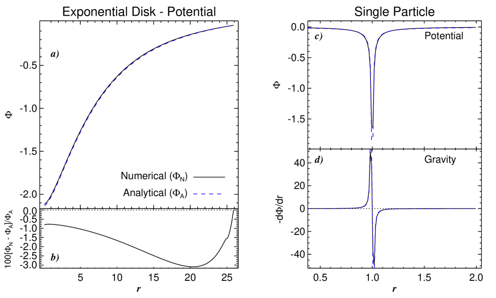
Figure 1: $a$. The potential generated by an exponential disk computed by Eq. (11) is compared with the analytical expression. The accuracy ($b$.) is at the percent level.
$c$. The potential generated by a single particle agrees very well with its Newtonian prediction. In particular, the scheme ensures that the gravity ($d.$) is smooth and the particle does not suffer self-acceleration.

We work in the thin disk approximation, using the vertically averaged equations of hydrodynamics

$$\frac{D\varSigma_{g}}{Dt} = -\varSigma_{g}{{\bm{\nabla}}\cdot{\bm{u}}}\ +\ f_{{}_{D}}(\varSigma_{g})$$ (1)

$$\frac{D{\bm{u}}}{Dt} = \ -\frac{1}{\varSigma_{g}}{\bm{\nabla}}{P}\ -\ {\bm{\nabla}}\varPhi\ -\ \frac{\varSigma_{p}}{\varSigma_{g}}{\bm{f}}_{d}\ +\ {\bm{f}}_{\nu}({\bm{u}},\varSigma_{g})$$ (2)

$$\frac{d{{\bm{v}}}_{p}}{dt} = -{\bm{\nabla}}\varPhi+{\bm{f}}_{d}$$ (3)

$$\frac{d{{\bm{x}}}_{p}}{dt} = {\bm{v}}_{p}$$ (4)

$$\varPhi = \varPhi_{\rm sg}-\sum_{i}^{n}{\frac{GM_{i}}{\sqrt{{\mathcal{R}}_{i}^{2}+b_{i}^{2}}}}$$ (5)

$$\nabla^{2}\varPhi_{\rm sg} = 4{\pi}G\varSigma\delta(z)$$ (6)

$$P = \varSigma_{g}c_{s}^{2}$$ (7)

$$f_{d} = -\left(\frac{3\rho_{g}C_{D}|\Delta{{\bm{v}}}|}{8a_{\bullet}\rho_{\bullet}}\right)\Delta{{\bm{v}}}.$$ (8)

In the above equations, $\varSigma_{g}$ and $\varSigma_{p}$ are the vertically integrated gas density and bulk density of solids, respectively. In Eq. (6), $\varSigma$ is their sum. ${\bm{u}}$ stands for the velocity of the gas parcels; ${\bm{v}}_{p}$ is the velocity of the solid particles, and ${\bm{x}}_{p}$ is their position; $P$ is the vertically integrated pressure, $c_{s}$ is the sound speed, $\varPhi$ the gravitational potential and ${\bm{f}}_{d}$ is the drag force by which gas and solids interact. In Eq. (8), $\rho_{\bullet}$ is the internal density of a solid particle, $a_{\bullet}$ its radius, and $\Delta{{\bm{v}}}={\bm{v}}_{p}-{\bm{u}}$ its velocity relative to the gas. The nature of the drag is concealed in the dimensionless coefficient $C_{D}$, discussed in section 2.2. The operator ${D}/Dt=\partial/{\partial}t+{\bm{u}}\cdot{\bm{\nabla}}$ represents the advective derivative.

The gravitational potential $\varPhi$ has contributions from the star, the giant planets, and the disk’s self-gravity. The star and the planets are treated as massive particles with a simple $N$-body code. In Eq. (5), $G$ is the gravitational constant, $M_{i}$ is the mass of particle $i$ and ${\mathcal{R}}_{i}=|{\bm{r}}-{{\bm{r}}}_{p_{i}}|$ is the distance relative to particle $i$. The quantity $b_{i}$ is the distance over which the gravity field of particle $i$ is softened to prevent singularities.

The function $f_{{}_{D}}(\varSigma_{g})$=$D_{3}\nabla^{6}\varSigma_{g}$ is a third order hyperdiffusion term. In Fourier space, it is proportional to $k^{6}$, where $k$ is the wavenumber. Being so, it behaves as a high-frequency filter, and is very effective in providing numerical stabilization near the grid scale while having little effect in the more quiescent larger scales. The function ${\bm{f}}_{\nu}({\bm{u}},\varSigma_{g})$ has both a hyperviscosity and a shock viscosity term

$${\bm{f}}_{\nu}({\bm{u}},\varSigma_{g}) = \varSigma_{g}^{-1}{\bm{\nabla}}\cdot{\left(2\varSigma_{g}\nu_{3}\mathbf{S}^{(3)}\right)}+$$ (9)

$$\zeta_{\nu}\left[{\bm{\nabla}}{({\bm{\nabla}}\cdot{{\bm{u}}})}+({\bm{\nabla}}{\ln\varSigma_{g}}+{\bm{\nabla}}{\ln\zeta_{\nu}}){\bm{\nabla}}\cdot{{\bm{u}}}\right]$$

where $S^{(3)}_{ij}$=$\partial_{j}^{5}u_{i}$ is a simplified (third-order) rate-of-strain tensor and the shock term $\zeta_{\nu}$ follows the formulation of Haugen et al. (2004), being proportional to the smoothed (over three grid cells in each direction) maximum (also over three grid cells) of the positive part of the negative divergence of the velocity, i.e.

$$\zeta_{\nu}=\nu_{\rm shock}\left<\max_{3}[(-{\bm{\nabla}}\cdot{\bm{u}})_{+}]\right>\left(\Delta x\right)^{2}.$$ (10)

The shock viscosity coefficient $\nu_{\rm shock}$ is a parameter of order unity. We use $\nu_{\rm shock}$=1 and $\nu_{3}$=$D_{3}$=$5\times 10^{-12}$. This hyperviscosity relates to the usual Laplacian viscosity by $\nu_{3}$=$\nu k^{4}$. Therefore, it corresponds to $\nu\simeq 3\times 10^{-3}$ (or $\alpha\simeq 1$) at the grid scale where $k$=$\pi/\Delta{x}$, and $\nu\simeq 10^{-11}$ ($\alpha\simeq 4\times 10^{-9}$) at the largest scale of the box. Here $\alpha$=$\nu\varOmega_{K}c_{s}^{-2}$ is the usual Shakura-Sunyaev viscosity parameter (Shakura & Sunyaev 1973) and $\varOmega_{K}$ the Keplerian frequency.

The simulations were done with the Pencil Code in Cartesian and cylindrical geometry. We write Cartesian coordinates as ($x$,$y$) and cylindrical coordinates as ($r$,$\phi$).

2.1 Self-gravity

We solve the Poisson equation Eq. (6) using the traditional rapid elliptic solvers with multiple Fast Fourier Transforms. For a single Fourier component $\widehat{\varSigma}$ the solution to Eq. (6) is

$$\widehat{\varPhi}=-\frac{2\pi{G}\widehat{\varSigma}}{|{\bm{k}}|},$$ (11)

where ${\bm{k}}=(k_{x},k_{y})$ is the in-plane wavenumber and the hat denotes Fourier transformed quantities. The potential is then found by taking the inverse transform to real space.

As the Fourier transform assumes periodic boundaries, the potential derived is as if the disk was accompanied by mirror images of itself, the gravity of these images influencing the motion of the fluid. To reduce this problem, we expand the grid by a factor 2 prior to solving the Poisson equation. In this expanded grid, the mirrors are still present, but they are now located so far away from the regions of interest that no spurious behavior is introduced by the periodic boundaries. We show in Fig. 1a the potential of an exponential disk, typical of galaxies, in which case the analytical solution is well known (Freeman 1970). The deviations are at the percent level, as seen in Fig. 1b.

The gravitational potential of the swarm of particles is found by the same method outlined above. The surface density of particles is assigned to the mesh using the Triangular Shaped Cloud (TSC) scheme (Hockney & Eastwood 1981, Youdin & Johansen 2007), whereby the influence of a particle is assigned to three grid points in each direction. After finding the potential, the acceleration is interpolated back to the position of the particles, using the same TSC scheme, to avoid self-acceleration (Johansen et al. 2007).

Analytical prediction and numerical solution for the potential of a single particle are compared in Fig. 1c. Deviations occur only near the particle position, as expected for a particle-mesh method. Fig. 1d shows the gravitational acceleration generated by this potential. The agreement is excellent and the particle does not experience any self-acceleration.

2.2 Drag force

Solid particles and gas exchange momentum due to interactions that happen at the surface of the solid body. The many processes that can occur are generally described by the collective name of “drag” or “friction”. The drag regimes are controlled by the mean free path $\lambda$ of the gas, which can be expressed in terms of the Knudsen number of the flow past the particle $\mathrm{Kn}=\lambda/(2a_{\bullet})$. High Knudsen numbers correspond to free molecular flow, or Epstein regime. Stokes drag applies at low Knudsen numbers. In this section we describe our numerical implementation of drag forces in the Pencil Code for general values of $\mathrm{Kn}$. We use the formula of Woitke & Helling (2003; see also Paardekooper 2007), which interpolates between Epstein and Stokes regimes

$$C_{D}=\frac{9\mathrm{Kn}^{2}C_{D}^{\rm Eps}+C_{D}^{\rm Stk}}{(3\mathrm{Kn}+1)^{2}}.$$ (12)

where $C_{D}^{\rm Eps}$ and $C_{D}^{\rm Stk}$ are the coefficients of Epstein and Stokes drag, respectively. They read

$$C_{D}^{\rm Eps} \approx 2\left(1+\frac{128}{9\pi\mathrm{Ma}^{2}}\right)^{1/2}$$ (13)

$$C_{D}^{\rm Stk} = \left\{\begin{array}[]{ll}24\,\mathrm{Re}^{-1}+3.6\,\mathrm{Re}^{-0.313}&\mbox{; $\mathrm{Re}\leq 500$};\\ 9.5\times 10^{-5}\,\mathrm{Re}^{1.397}&\mbox{; $500<\mathrm{Re}\leq 1500$};\\ 2.61&\mbox{; $\mathrm{Re}>1500$}.\end{array}\right.$$ (17)

where $\mathrm{Ma}=|\Delta{{\bm{v}}}|/c_{s}$ is the Mach number, $\mathrm{Re}=2a_{\bullet}\rho_{g}|\Delta{{\bm{v}}}|/\mu$ is the Reynolds number of the flow past the particle, and $\mu=\sqrt{8/\pi}\rho_{g}c_{s}\lambda/3$ is the kinematic viscosity of the gas.

The approximation for Epstein drag (Kwok 1975) connects regimes of low and high Mach number ($\mathrm{Ma}=|\Delta{{\bm{v}}}|/c_{s}$) to good accuracy, and is more numerically friendly than the general case (Baines et al. 1965). The piece-wise function for the Stokes regime are empirical corrections to Stokes law ($C_{D}=24\mathrm{Re}^{-1}$), which only applies for low Reynolds numbers.

Fig. 2a shows the value of this coefficient in the plane of Mach and Knudsen numbers. As stressed by Woitke & Helling (2003), at intermediate Knudsen numbers, the true friction force yields smaller values than in both limiting cases, which is illustrated in Fig. 2b. Another measurement of the strength of the drag force is the friction time $\tau_{{}_{f}}$, defined as the inverse of the quantity in parentheses in Eq. (8)

$$\tau_{{}_{f}}=\frac{4\lambda\rho_{\bullet}}{3\rho_{g}C_{D}c_{S}}\frac{1}{\mathrm{Ma}\mathrm{Kn}}.$$ (18)

The drag acceleration can then be cast in the compact form

$$f_{d}=-\frac{1}{\tau_{{}_{f}}}\Delta{{\bm{v}}_{p}}.$$ (19)

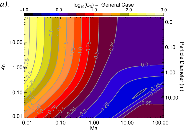
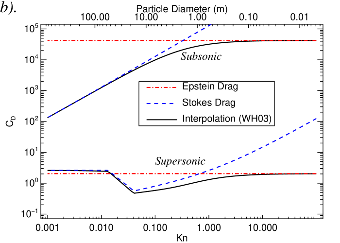
Figure 2: The interpolated general drag coefficients in a). the plane of Knudsen and Mach numbers. In b). we show two slices at subsonic and supersonic motion, comparing to the respective predictions of Epstein and Stokes drag. For particles up to 10 centimeters, Epstein drag does not deviate much from the general (interpolated) coefficient. Pure Stokes drag starts to apply only beyond 10 meters.

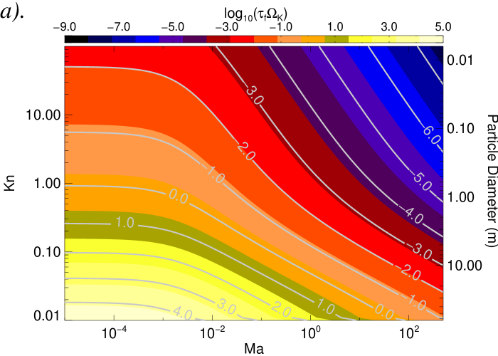
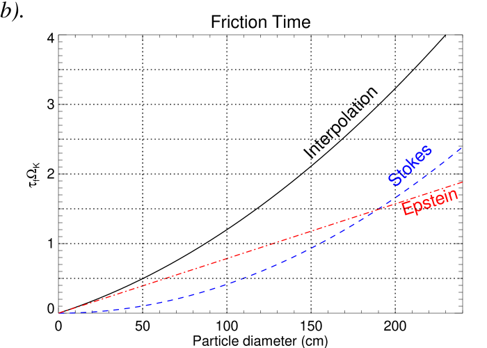
Figure 3: a). The drag coefficient translated to friction times for our choice of numerical parameters at Jupiter’s orbital position. In b). we show a slice of a). at subsonic regime, where the predictions of Epstein and Stokes law are shown for comparison. The general drag yields more loose coupling than both limiting cases.

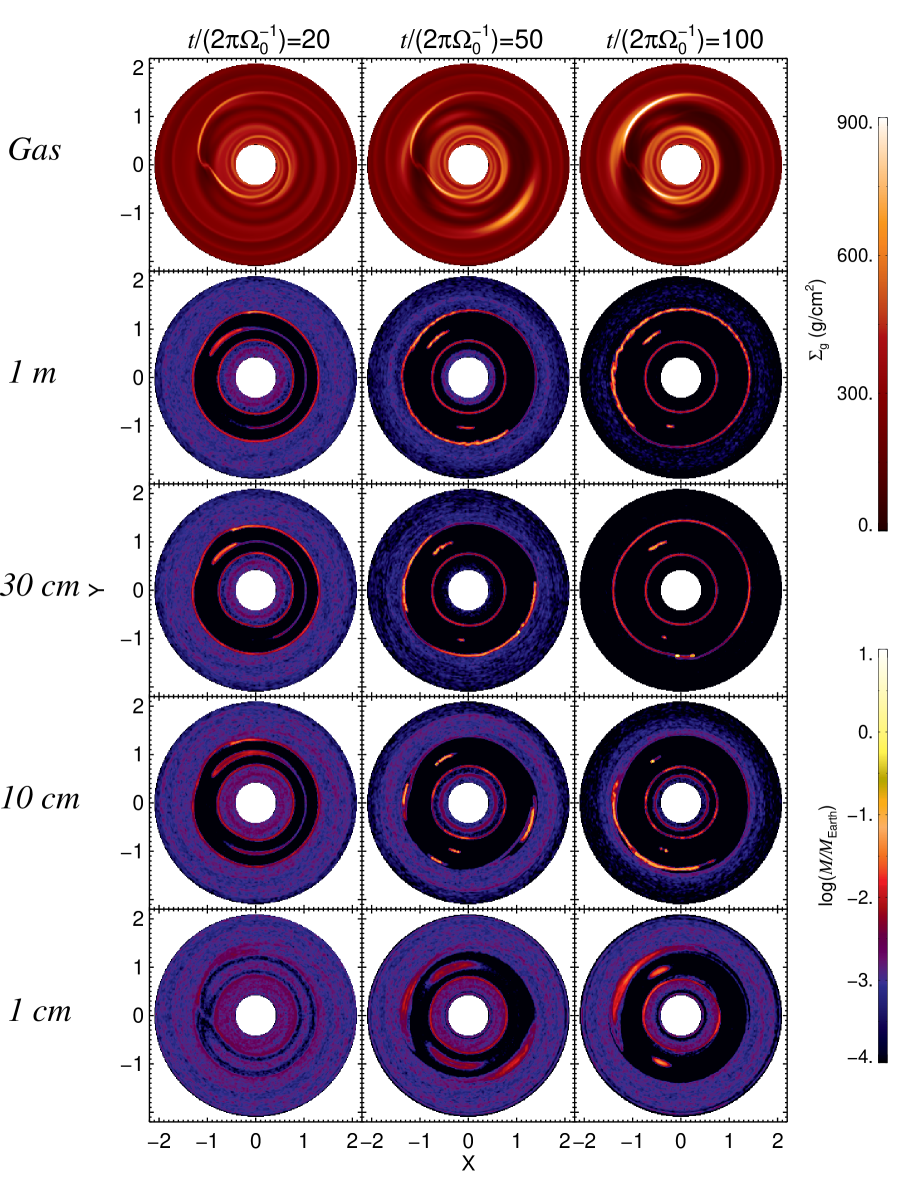
Figure 4: Snapshots of the gas and solid phase of the disk for several single particle species runs, for a perturber of Jupiter’s mass. At the end of the simulations at 100 orbits, the swarms of particles in the L4 and L5 points of the $a_{\bullet}$=1 m run remain unbound. The 10 cm and 30 cm particles underwent collapse at the Lagrangian points, with the fragmentation being more efficient for the 10 cm particles than for the 30 cm ones. In the $a_{\bullet}$=10 cm case, the particles underwent collapse in both Lagrangian points, L5 harboring a 2.6 $M_{\oplus}$ planet, L4 a 0.6 $M_{\oplus}$. At the edges of the gap, even $a_{\bullet}$=1 cm particles are trapped within the vortices. In the $a_{\bullet}$=10 cm run, the effect of the anti-cyclonic motion lead to a final collapsed mass of 0.3 $M_{\oplus}$. When the vortices merge into a single giant vortex, the $a_{\bullet}$=30 cm particles are seen to have undergone runaway growth of solids, reaching 17 $M_{\oplus}$.

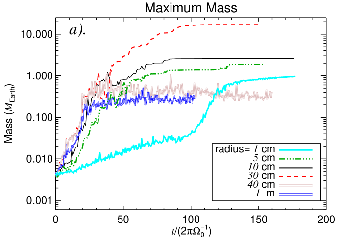
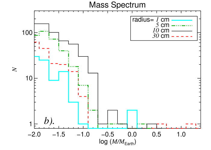
Figure 5: a). Time evolution of the maximum concentration of mass for different particle radii. From 40 cm onwards, the drag force is too weak to provide enough damping for collapse. For 1 cm to 30 cm radii, gravitational collapse occurs forming Earth-mass planets. For 5 cm, a 2 $M_{\oplus}$ planet is formed. For 10 cm, the final maximum collapsed mass is around 3 $M_{\oplus}$. The particles of 30 cm radius collapse in a planet as massive as 17 Earths. The $a_{\bullet}$=1 cm are subject to strong coupling and undergo growth on the timescale of depletion of gas in the Lagrangian points. This leads to a delay in the collapse, taking twice the time it took in the 5-30 cm case. The final mass is 1 $M_{\oplus}$.
b). The mass spectrum in the end of the simulations. Along with the super-Earths formed with the 30 cm, 10 cm and 5 cm particles, dozens of Mars sized and hundreds of Moon sized objects were also formed. The two symmetric Trojan Earths in the 1 cm case are apparent. The runs with particles of $a_{\bullet}$=40 cm and $a_{\bullet}$=1 m were excluded for clarity.

2.3 Initial conditions

We use a Cartesian box ranging $x,y\in[-2.0,2.0]r_{0}$, with resolution 256$\times$256. The small extent in radius is justified because we want to understand what is happening at the vicinity of the planet’s orbit at $r_{0}$ and the gap it opens. The density profile follows the power law $\varSigma_{g}$=$\varSigma_{0}r^{-0.5}$ and the sound speed is also set as a power law $c_{s}=c_{s_{0}}r^{-0.5}$.

The gravitational potential is then computed via the Poisson solver and the initial velocity profile is set to match the condition of centrifugal equilibrium

$$\dot{\phi}^{2}=\varOmega_{\rm K}^{2}+\frac{1}{r}\left[\frac{1}{\varSigma_{g}}\frac{\partial{P}}{\partial{r}}+\frac{\partial{\varPhi_{\rm sg}}}{\partial{r}}\right]$$ (20)

The planet is placed initially at ($r$,$\phi$)=($r_{0}$,0), and the star at ($r$,$\phi$)=(0,$\pi$). To avoid giving the gas and the particles too much impulse when the planet is introduced in the unperturbed disk, we ramp its mass up from 0 to its final mass in five orbits, in the way described in de Val-Borro et al. (2006). We computed simulations with companion mass ratios $q$=$10^{-3}$ (Jupiter) and $q$=$10^{-4}$ (“Neptune”). The quotation marks are used because calling this mass ratio “Neptune” is a jargon, since the actual mass of the planet is the equivalent to $q$=$5\times 10^{-5}$. The Earth has a mass ratio of $q$=$3\times 10^{-6}$.

We use units such that $r_{0}$=$\varSigma_{0}$=$GM_{\odot}$=1. We choose $c_{s_{0}}=0.05$ and a Toomre $Q$ parameter of 30 at the position of the planet, so the gas there is stable against gravitational instability. Assuming that $r_{0}$ is the position of Jupiter (5.2 AU) and that $\varSigma_{0}$=300 g cm^-2, the disk has $10^{-2}M_{\odot}$ of gas within the modeled range.

For the solids, we use $10^{5}$ Lagrangian numerical particles, and the interstellar solids-to-gas ratio of $10^{-2}$. Each numerical particle therefore is a super-particle containing $10^{-9}M_{\odot}\simeq 3\times 10^{-2}M_{\rm Moon}$ of material. The super-particle formalism considers that each numerical particle is an ensemble of a large number of individual smaller physical particles of radius $a_{\bullet}$. These particles share the same position and velocity, interacting gravitationally by their collective mass (the mass of the super-particle). The aerodynamics, however, is controlled by the radius $a_{\bullet}$, which in turn means that there is free space between the physical particles, so that each of them exposes its whole surface area to the nebular gas.

We stress that the mass resolution of solids in the models presented in this paper is not much greater than that used by Beaugé et al. (2007). The main difference between this study and theirs lies in the global character of our study; the greater number of numerical particles; and the radius $a_{\bullet}$ of the individual pebbles and boulders, which translates into a much stronger drag force.

We survey several particle radii. The dimensionless friction time as a function of particle size is found by plugging Eq. (12) into Eq. (18), which yields

$$T_{{}_{f}} = \tau_{{}_{f}}\varOmega_{K}$$ (21)

$$= \frac{\sqrt{32\pi}}{\mathrm{Kn}^{\prime}\mathrm{Ma}}\frac{\lambda\rho_{\bullet}}{\varSigma_{g}}\frac{(\mathrm{Kn}^{\prime}+1)^{2}}{\left(\mathrm{Kn}^{\prime 2}C_{D}^{\rm Eps}+C_{D}^{\rm Stk}\right)}$$

where we already substituted $\rho_{g}$=$\varSigma_{g}/(\sqrt{2\pi}H)$. Here, $H=c_{s}/\varOmega_{K}$ is the pressure scale height. We consider that the particles have an internal density $\rho_{\bullet}$=3 g cm^-3. The mean free path $\lambda$ is

$$\lambda=\frac{\mu_{\rm mol}}{\rho_{g}\sigma_{\rm mol}}$$ (22)

where $\mu_{\rm mol}=3.9\times 10^{-24}$ g is the mean molecular weight of a 5:1 H₂-He mixture, and $\sigma_{\rm mol}=2\times 10^{-15}$ cm² is the cross section of molecular hydrogen. For our densities and sound speed, it corresponds to 20 cm at the inner radius $r$=0.3, and to 1.3 m at the outer radius $r$=2.0.

The result of Eq. (21) for our choice of parameters (at the position of Jupiter’s orbit) is shown in Fig. 3a for the grid of Knudsen and Mach numbers. Fig. 3b shows a slice of the grid at the subsonic regime. For particle of 1m diameter, the coupling due to Eq. (21) is 50% looser than predicted by Epstein law. A factor 2 in the friction time is seen at 2m diameter between Eq. (21) and the Stokes law.

The particles are initialized as to yield a surface density following the same power law as the gas density, and their velocities are initialized to the Keplerian value.

We use reflective boundaries and damp waves in the way described in de Val-Borro et al. (2006). Particles are removed from the simulation if they cross the inner boundary or if they approach the giant planet by less than 1/5 of its Hill’s radius.

3 Simulations with single particle species

In Fig. 4 we show the time evolution of the disk under the influence of a $q$=$10^{-3}$ companion, for different particle radii. Each run has only one particle size, but as the gas density does not change significantly between the runs, we just show the gas for the $a_{\bullet}$=1 cm case.

3.1 Collapse in the Lagrangian points L4 and L5

As the planet opens a gap in the gas, the particles also move out of the co-rotational region, in the same manner seen in Paardekooper (2007) and Fouchet et al. (2007). The solids at the border of the gap are expelled and those in the immediate vicinity of the planet are accreted. The particles inside the co-rotational region librate in horseshoe orbits. The stable leading (L4) and trailing (L5) Lagrangian points retain high gas densities even after the planet has carved a deeper gas gap in its orbit, which has a beneficial effect for the particle concentration. Due to the presence of high gas densities, the Lagrangian islands are not only a region of convergence of streamlines, but also a region with higher pressure than its surroundings. The drag force therefore forces the particles into them, also damping the motion caused by eventual perturbations that could otherwise make a particle drift away from it. These effects combined make L4 and L5 highly stable points in the motion of a solid particle.

At 20 orbits, an asymmetry is seen in the particle concentration between L4 and L5, as the trailing Lagrangian point is more efficient in trapping than the leading one. The 10 cm, 30 cm and 1 m particles achieve high concentrations in the vicinity of L5, while experiencing depletion in L4. The 1 cm particles are too coupled to the gas to be affected by particle-gas drift.

At 50 orbits, the concentration in the Lagrangian points has increased by two orders of magnitude relative to the initial condition in the 10 cm, 30 cm and 1 m runs. The particles of 10 cm and 1 m still present an azimuthally extended cloud of material in L4 and L5, but the particles of 30 cm radii have already concentrated into a small swarm spanning but a few grid cells. Inspection of the snapshot reveals that the maximum mass in this swarm is of 0.03 $M_{\oplus}$. The L4 concentration is more extended, but the maximum density is greater, achieving 0.25 $M_{\oplus}$, already exceeding the mass of planet Mars (0.1  $M_{\oplus}$).

At the end of the simulation at 100 orbits, the swarms of particles in the L4 and L5 points of the $a_{\bullet}$=1 m run remain unbound. We ran for additional 50 orbits, but no progress in the maximum mass was seen. If collapse happens, it requires timescales longer than 150 orbits. The total mass in L4 is 0.29 $M_{\oplus}$, peaking at 0.05. The L5 point has 1.9 $M_{\oplus}$ in total, with maximum mass concentration of 0.3 $M_{\oplus}$. The 10 cm and 30 cm particles underwent collapse at the Lagrangian points, with the gravitational fragmentation being more efficient for the 10 cm particles than for the 30 cm ones. For the $a_{\bullet}$=30 cm case, what appears in Fig. 4 as a single clump at L4 has a mass of 0.18 $M_{\oplus}$. The L5 point is still azimuthally extended, with a total mass of 2.5 $M_{\oplus}$ but maximum concentration of only 0.27 $M_{\oplus}$ by the end of the simulation.

The $a_{\bullet}$=10 cm particles underwent collapse in both Lagrangian points, L5 harboring a 2.6 $M_{\oplus}$ planet, L4 a 0.6 $M_{\oplus}$. In Fig. 5a we plot the time evolution of the maximum mass of solids for different runs. In addition to the runs showed in Fig. 4 we add runs with particles of 5 cm and 40 cm radii. Collapse in the Lagrangian points occurs for the 5 cm case as well, forming a planet of 2 $M_{\oplus}$. In this figure, the difference between a run where collapse occurred and a run where collapse did not occur is readily apparent by the behavior of the time-series. The non-collapsed ones are very noisy at late times, as the number of particles in a cell fluctuates up and down. When collapse is achieved, the maximum mass stays constant unless more mass is accreted. This gives the time series a ladder-like appearance, as seen in the figure for the 5,10, and 30 cm cases. Collapse is hindered for $a_{\bullet}$=40 cm onwards.

The 1 cm particles present an interesting behavior. They are so strongly coupled to the gas that their collapse does not occur at the same time-scale, as seen from Fig. 5a. Instead, as Fig. 4 evidences, it occurs on the timescale of depletion of gas in the tadpole orbits. As the gap is cleared and its depth increases, the gas clouds in the Lagrangian islands shrink in size. As the particle are strongly coupled, they are forced to concentrate as the cloud shrinks, eventually achieving high densities. As the time series of Fig. 5 shows, after 100 orbits the steady increase due to gas clearing gives place to a runaway growth that lasts for about 20 orbits. In the end, one gravitationally bound planet encerring one Earth mass of solids - purely out of 1 cm sized pebbles -, is formed in each stable Lagrangian point.

3.2 Collapse at the gap edge vortices

Concurrently, at the edges of the gap, the considerable density gradient resulting from the gap opening process excites the RWI, leading to a large generation of potential vorticity. At fifty orbits, two vortices are seen to have been excited by the planet at the outer edge of the gap, seen in Fig. 4 at 5 and 10 o’clock. The effect of these vortices in the motion of the solids can be readily seen in the $a_{\bullet}$=1 cm run, as even for these tightly coupled particles, the concentration reaches an order of magnitude higher than in the immediate surroundings.

In the $a_{\bullet}$=10 cm run, as the particles are more loosely coupled to the gas, the effect of the anti-cyclonic motion is better appreciated. The particles are forced in spiral trajectories towards the center of the vortices, raising the density of solids by another order of magnitude when compared to the $a_{\bullet}$=1 cm particles.

In the $a_{\bullet}$=30 cm and $a_{\bullet}$=1 m runs, the coupling is too loose to form the extended structure seen for the $a_{\bullet}$=1 cm and 10 cm particles. However, the looseness is a benefit as long as the goal is to increase the concentration of solids. As the coupling weakens, the particles are not forced away from the center, and concentrate more efficiently. A massive clump of particles is seen in the 4 o’clock vortex in the $a_{\bullet}$=30 cm run, that already concentrates 2 $M_{\oplus}$ of solid material. High particle concentration is also seen for the $a_{\bullet}$=1 m particles, but they do not seem to get dense enough to achieve gravitational collapse. Instead, they form a very azimuthally extended belt of particles at the outer and inner edge. No collapse is seen at the inner edge of the gap in any of the runs. At 100 orbits, the vortices have merged into a single giant vortex. Inside it, in the 30 cm run, the collapsed mass underwent runaway growth of solids, reaching 17 $M_{\oplus}$. The 10 cm particles have a maximum mass in the vortex of 0.3 $M_{\oplus}$. The 1 m particles show a similar maximum mass, of 0.25 $M_{\oplus}$. The high mass achieved in the 30 cm run is quite likely overestimated, since it is seen that the efficient and unimpeded particle drift had the effect of feeding this radial region with virtually all particles present in the simulation. Such a situation may be made quite different in a more realistic case, where particle drift is stalled by turbulence, for instance.

In Fig. 5b, we show the mass spectrum at the end of the different simulations. In addition to the super-Earths, two planets in the 0.5-0.8 $M_{\oplus}$ range were formed out of 5 cm particles, and other two in the 0.3-0.5 range with the 30 cm particles. Dozens of Mars-sized planets in the 0.08-0.3 $M_{\oplus}$ range, along with hundreds of smaller Moon-sized objects, were also formed in all simulations.

4 A spectrum of particle sizes - segregation and the counter-intuitive role of self-gravity

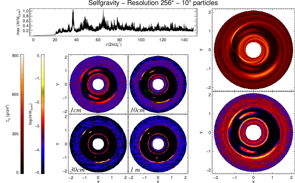
Figure 6: Comparison between the runs with resolution $256^{2}$, $10^{5}$ particles and multiple particle species, with and without self-gravity (upper and lower panels, respectively). Counter-intuitively, self-gravity is seen to work against collapse as in the second run the maximum mass is never high enough to allow it. In the presence of self-gravity, the tadpole orbits are modified, and gas tides from the massive vortices can be disruptive for planets forming within them. The motion of the particles inside the vortices are also modified in the presence of self-gravity. Notice in particular how the 30 cm and 1 m particles are spatially split in the vortex at 10 o’clock, near L5. Collapse proceeds only if the grid resolution is refined (see text and Fig. 7.)

To understand the effect of self-gravity in the runs, we perform a control run with only gas drag. To diminish the computational time, we include in this run a spectrum of particles radii, including four species: 5, 10, 30, and 100 cm. Each particle species is represented by 1/4 of the total number of particles. To compare with this non-selfgravitating run, we also compute a self-gravitating run with a size spectrum. These runs not only shed light onto the role of self-gravity, but can also discern the possible artificial effects introduced by the single-species approximation used by us so far.

4.1 Excluding self-gravity: gas drag alone assembles super-Earths

In Fig. 6a we show the time evolution of the maximum mass in the non-selfgravitating run, along with the disk appearance in the gas phase as well as the contribution of each particle species in the solids phase. As stated before, the drag provides a very efficient damping, so that the particles of all species except 1 cm concentrate in the L4 and L5 as well as in vortices as early as 50 orbits. The 30 cm and 1 m particles successfully concentrate all its remaining particles that lie in the co-orbital region in a single cell in each of the stable Lagrangian points. The 30 cm particles concentrate with 0.66 $M_{\oplus}$ in L5 and 0.04 in L4; the 1 m particles with 0.54 $M_{\oplus}$ in L5 and 0.1 in L4. The concentration of 10 cm particles is less efficient, with a maximum concentration of only 25% of the particles in L5 (which nonetheless means 0.13 $M_{\oplus}$). Of the 2.1 Earth masses of material in L5, the representation is 0.25 $M_{\oplus}$ in 1 cm particles, equal shares of 0.66 $M_{\oplus}$ of 10 and 30  cm, and 0.54 $M_{\oplus}$ of 1 m particles. The L4 point has 0.55 $M_{\oplus}$, distributed 0.23, 0.17, 0.04, and 0.1 $M_{\oplus}$ for 1, 10, 30, and 100 cm, respectively.

At the outer edge of the gap, as more material is available, the concentration achieves higher masses. Without self-gravity, the clumps cannot collapse, quickly dispersing and regrouping instead. The maximum mass then is highly fluctuating. After 60 orbits, it has grown to 2 Earth masses, but sporadicly reaching as high as 6 $M_{\oplus}$, due to gas drag alone. The vortex closest to L5 seen in Fig. 6, a snapshot at 62 orbits, concentrates 2.9 $M_{\oplus}$ in the densest cell. The 1 m particles have a maximum concentration of 2.75 $M_{\oplus}$, similarly to the 30 cm ones, which peak at 2.3 $M_{\oplus}$. It shows that the different particle species preferentially concentrate in different cells, a result of the different drag they feel. The same was seen in the Lagrangian points. The 10 cm is more extended, peaking at 0.1 $M_{\oplus}$, a relatively low mass. The leading vortex presents the same qualitative behavior, with a peaking mass of 1.64 $M_{\oplus}$, 10, 30, and 100 cm particles showing highest concentration of 0.3, 1.3 and 1.25 $M_{\oplus}$, respectively.

4.2 Including self-gravity: collapse hampered

When self-gravity is considered (Fig. 6b), the accretion is seen to be stalled. Sparse episodes of high particle concentration happen at $\sim$38 and 65 orbits, reaching maximum masses of 1 $M_{\oplus}$, but the collapse of this mass did not occur and the clump quickly dispersed. After a hundred orbits, the maximum mass was still at the 0.2 $M_{\oplus}$ level. The L4 point was cleared of particles compared to the non-selfgravitating run, displaying 0.7 $M_{\oplus}$ of solid material, more than half of it in 1 cm particles. The highest concentration is of 0.19 $M_{\oplus}$, which is mostly represented by 10 cm particles, contributing 0.17 $M_{\oplus}$, 100% of the 10 cm particles remaining in the L4 vicinity. The totality of 30 cm particles in the region are also concentrated in a single cell, but its mass is of only 0.04 $M_{\oplus}$, and although spatially close to the 0.17 $M_{\oplus}$ clump of $a_{\bullet}$= 10 cm, they are not at the same cell. The 1 m particles still show a slightly extended cloud, with total mass 0.1 $M_{\oplus}$, some degrees away from both 10 cm and 30 cm concentrations. The tadpole of particles around L5 is still highly extended spatially. We ran the simulation for additional 50 orbits, but the conditions remained unchanged. In particular, the 3 nearby clumps of different particle species did not collapse into a single body.

There are four reasons as to why collapse did not proceed as in the single species runs. First, the mass of solids was equally split in particles of different size. The 1 cm particle retain 1/4 of the mass, and they concentrate very poorly due to their short friction time. This mass is thus effectively removed from the mass of potentially collapsable bodies. Running for longer times to allow the shrinking Lagrangian gas clouds to squeeze the 1 cm particles into a collapsed body (as occurred in the single species $a_{\bullet}$=1 cm run after 150 orbits) did not produce the same results, as seen in the time series in the lower panels of Fig. 6.

Second, the gravitational potential of the massive particles acts to de-stabilize the Trojan orbits. As the mass in the Lagrangian points grow, the massless approximation ceases to apply, and the body starts to librate around the otherwise stable point. As the mass increases, the librations increase in amplitude and lead the other particles into close encounters with the giant, that are thence accreted or ejected from the system. In the limiting case that the mass of the Trojan body becomes comparable to the mass of the planet itself, the amplitude of libration would become so high that an encounter between the two would occur. Beaugé et al. (2007) find that a 0.15 $M_{\oplus}$ object is enough to de-stabilize the orbits of other bodies in the vicinity of L4.

The effect of this libration in our simulations is evident when comparing Fig. 6a and Fig. 6b. Instead of concentrating at L4 and L5 as the massless particles do, the massive particles display an azimuthally extended structure, evidence of the enhanced librating motion.

Third, the inclusion of gas gravity leads to tides that can be disruptive for a prospective planet (Lyra et al. 2008b). In a simple yet informative approximation, the tides can be taken as proportional to the radius $R$ of the clump and to the gradient of the gravitational acceleration which, by the Poisson equation, is proportional to the local value of the density, $F_{T}\propto R\rho_{g}$. For a spherical clump of constant density $\rho_{p}=3M_{p}/(4\pi R^{3})$, the self-gravitational pull it exerts on its own surface is $F_{G}$=$GM_{p}/R^{2}\propto R\rho_{p}$. The ratio $F_{T}/F_{G}$ is therefore proportional to the gas-to-solids ratio. For a protoplanet forming inside high-pressure regions such as vortices or the Lagrangian clouds, the gas tides can lead to destruction or significant erosion of the forming planets (Lyra et al. 2008b).

Fourth, a common feature of all simulations is that the particles of different radii tend to concentrate in different locations within the tadpole region. This is somewhat similar to the effect of self-gravity. Gas drag taps energy from the Keplerian motion, so the stability conditions on the Lagrangian points are modified. As gas drag depends on radius, the location of the stable points of the 3-body problem with gas drag also depend on particle size. In other words, the L4 and L5 points of the restricted 3-body problem are defined as points where there is a balance between the gravitational attraction between the 2 massive bodies and the centrifugal force. When including gas drag, a third force comes into play in the particle motion, and the stable points will be displaced accordingly. In general, a particle of a given size will librate about its own particular stationary point. Numerical and analytical investigations by Peale (1993) and Murray (1994) confirm that the location of the stable points is a function of particle radius. Asymmetries between L4 and L5 are also expected from the analytical treatment, which are seen in our simulations as well, with L4 shifting further away than 60^∘ ahead of the planet, while L5 is displaced closer behind it. In some extreme cases, the stable points can vanish altogether. As the drag force increases and L5 approaches the planet, it can merge with the shifted L2 point. L4 experiences the same as it moves further out and merges with the shifted L3 point. Both Murray (1994) and Peale (1993) find a limiting location of 108^∘ ahead of the planet for L4. At this maximum angular separation, the merging with L3 takes place and the leading stationary point disappears. For a 13 $M_{\oplus}$ proto-Jupiter, Peale (1993) finds that L4 does not exist for objects smaller than $a_{\bullet}$=15 m. L5 is seen to be more stable, but the stable point of a $a_{\bullet}$=50 cm particle is expected to lie only a few degrees behind the proto-Jupiter. In this location, they speculate, the wake of the planet (not taken into account in their model) might effectively eliminate L5.

Increasing the mass of the perturber to that of Jupiter’s present mass tends to increase stability and to bring L4 and L5 closer to the “classical” locations predicted by the restricted 3-body problem. In a gap homogeneously depleted by 1 order of magnitude relatively to the initial density, the shift for the 10 m particles is less than 2^∘. However, the analysis of Peale (1993) and Murray (1994) did not consider the presence of higher gas densities in the (classical) Lagrangian points as the gap is cleared. As we see, it has an effect similar to a potential well, keeping the particles around the classical tadpole. As the 1 cm particles have shorter friction time, the gas trap is more efficient, and the prediction of their particular L5 getting too close to the planet, or L4 merging with L3 is avoided as long as a local pressure maximum is present at the classical L4 and L5. The more loosely coupled 1 m particles had their L4 shifted to 90^∘ ahead of the planet, and L5 to 50^∘ behind it.

5 Resolution study

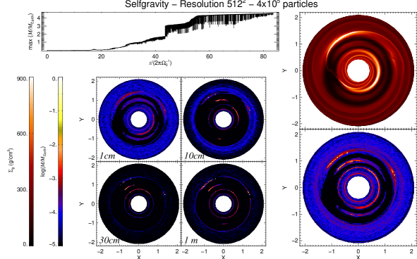
Figure 7: Results of the high-resolution run ($512^{2}$ grid points and $4\times 10^{5}$ particles) with multiple particle species. Four rocky planets form at the outer edge of the gap, the most massive one with 4.5 $M_{\oplus}$. They are easily spotted in the solids plot as very bright small dots. A movie of this simulation can be found at http://www.astro.uu.se/$\sim$wlyra/planet.html

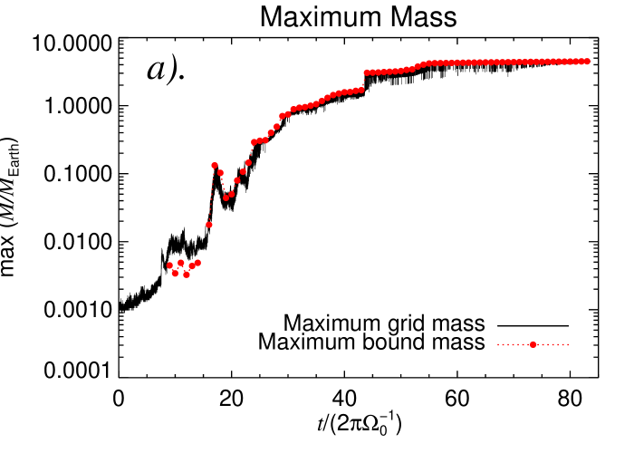
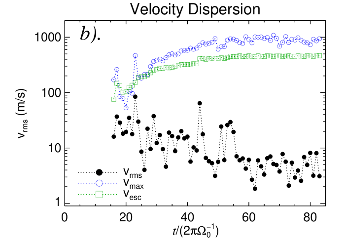
Figure 8: Time-series of the most massive clump present in Fig. 7. a). The maximum mass in a grid cell and the maximum bound mass. Even though the Hill’s radius exceeds the dimension of a grid cell, the planet has most (or all) of its mass within a single cell. This is evidence of subgrid compactness.
b). The internal velocity dispersion $v_{\rm rms}$  of the planet, compared with its escape velocity $v_{\rm esc}$  defined at the Hill’s radius. Throughout most of the simulation, $v_{\rm rms}$is below 10 m s^-1. The maximum internal speed is plotted for comparison. It usually exceeds the escape velocity, so some particles are not bound to the planet.

Motivated by the failure of the run just presented above to assemble massive gravitationally bound structures, we explore the effects of particle and grid resolution in our simulations. We first raise the total number of particles to $N_{p}$=400 000, to verify the effect of particle resolution. The mass of the disk is the same, so the mass of an individual super-particle decreases, being now $2.5\times 10^{-10}M_{\odot}\simeq 7\times 10^{-3}M_{\rm Moon}$. This first run has the same grid resolution as used before, 256². The second is twice as fine, 512².

The $N_{\rm x}\times N_{\rm y}$=256² and $N_{p}=4\times 10^{5}$ run does not show major differences when compared to the simulation with same resolution but only $10^{5}$ particles. The same behavior of sparse episodes of high concentrations but never achieving critical densities is seen. At the end of the simulation, the maximum mass is still around only 0.2 $M_{\oplus}$. We conclude from this that changing the particle resolution by at least a factor 4 does not change the results significantly.

On the other hand, the situation changes considerably when changing the grid resolution. In the run with $N_{\rm x}\times N_{\rm y}$=512² and $N_{p}$=$4\times 10^{5}$ (Fig. 7), the maximum mass steadily increases towards 1 $M_{\oplus}$ in 30 orbits. Inspection of the snapshots reveals that this high concentration occurs inside the vortices excited in the outer gap. At fifty orbits, the leading vortex shows two planets, one of 1.43 $M_{\oplus}$, and a smaller one of 0.38 $M_{\oplus}$. Unlike the 256² run, the mass peaks of different particles species occur at the same cell, attesting to the boundness of the structures. The first planet is 57.6% composed of 30 cm particles, 35.0% of 10 cm, 6.5% of 1 m and 0.9% of 1 cm particles. The second is 87% composed of 30 cm particles, about equal shares (6.5%) of 10 cm and 1 m particles, with only trace amounts of 1 cm particles.

The trailing vortex also shows two gravitationally bound planets, both of high mass. The most massive one has 3.1 $M_{\oplus}$, its composition of 1, 10, 30, and 100 cm particles being 0.2%, 17.9%, 63.0%, and 18.9%, respectively. The other planet is of 1.9 $M_{\oplus}$, being constituted by 0.2%, 27.8%, 48.9%, and 23.1% of 1, 10, 30, and 100 cm, respectively.

A common trait of these planets is, therefore, that they are formed by a majority of 30 cm particles, with approximately equal shares of 10 cm and 1 m particles. This is expected, since for our choice of parameters, the 30 cm particles are those for which the drift due to gas drag is maximum. The 1 cm are too well coupled to the gas to contribute significantly to the growth of terrestrial planets inside the vortices. For reasons of load imbalance, we terminated the simulation at 83 orbits, when a large fraction of the computational time was idle and one orbit took 6 hours in 64 processors. The most massive planet had grown to 4.5  $M_{\oplus}$ by then. The other planets formed at the outer edge of the gap show masses of 4.36, 4.14, and 0.80 Earth masses.

In Fig. 8a we show the time evolution of the mass of this massive planet. The black solid line represents the maximum mass of solids contained in a single grid cell. The red dashed line marks the maximum mass that is gravitationally bound. We decide for boundness based on two criteria. First we consider the clump defined by the black line, and calculate the center of mass of its particles. The Hill’s sphere associated with this mass is drawn, centered on the center of mass. As the Hill’s sphere encompasses more/less than a grid cell, particles inside/outside are added/removed from the total mass, and the center of mass and Hill’s radius recomputed. The process is iterated until convergence. After the clumps’ mass and Hill’s radius are defined, we compare the internal velocity dispersion $v_{\rm rms}$  of its constituent particles with the escape velocity of the enclosed mass, defined at the Hill’s radius. If $v_{\rm rms}$$<$ $v_{\rm esc}$, we consider that the cluster of particles is gravitationally bound. As seen in Fig. 8b, the internal velocities are usually lower than 10 m s^-1. We also plot the maximum speed and escape velocity of the planet (defined at the Hill’s radius). The maximum speed is usually greater than the escape velocity, which means that not all particles present in the cluster are actually bound, and the planet (as we define it) can lose mass during the accretion process. However, the low $v_{\rm rms}$  compared to $v_{\rm esc}$  attests that the vast majority of the particles is gravitationally bound.

At the end of the simulation, the gas in co-rotation is still spread over the whole horseshoe region, so a massive loss of particle from L4 is observed. The same process was seen in the other runs, with single and/or multiple species. But in this case, the effect is more severe as the L4 point of the 30 cm particles disappeared. At the end of the simulation, a small cloud of 2 $M_{\rm Mars}$ of 10 cm particles is observed in the tadpole region around L4, peaking at a maximum mass of 3.5 $M_{\rm Moon}$. L5 presents 3.3 $M_{\oplus}$ of solid material, but still in extended clouds. The boundness analysis shows that these clouds are fragmented into $\approx$20 sub-Mars sized bodies of mass between 1-5 lunar masses.

6 Neptune-mass perturber

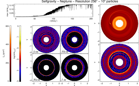
Figure 9: Same as Fig. 7 but for a Neptune-mass perturber. The Lagrangian point L4 has vanished and the L5 shifted to a position much nearer to the planet than in the Jupiter case. The wake of the planet does not destroy the stability of the shifted L5, and a Trojan of 1.6 $M_{\rm Mars}$ was formed.

In this section, we consider the case of a giant planet perturber of mass ratio $q$=$10^{-4}$, dubbed “Neptune”. This case is important to assess since, according to our current understanding, a forming gas giant is expected to spend a long time (of the order of millions of years) with a mass similar to this value - corresponding to the phase II of the model of Pollack et al. (1996). Even models that predict a faster transition from Neptune to Jupiter mass (Klahr & Bodenheimer, 2006) still predict timescales of ($\sim$10⁵ years). Therefore, when the perturber has achieved Jupiter’s mass, the state of the solids subdisk should be more similar to the state left by a Neptune-mass perturber than to the unperturbed disk of particles we have used so far.

We observe that when the perturber has a smaller mass, a more pronounced asymmetry between the L4 and L5 point is observed, as expected from the analysis of Peale (1993) and Murray (1994). The 1 m and 30 cm sized particles experience more depletion, with their L4 point having vanished altogether and the L5 shifted to but a few degrees behind the planet (Fig. 9). The 10 cm particles also experience depletion but not as severe as the larger particles. The 1 cm particles are well coupled and remain in co-rotation as no deep gas gap is carved.

The shifted L5 points of the 30 cm and 1 m particles concentrate about only 0.01  $M_{\oplus}$ of solids, each. Nevertheless, a Trojan planet of 0.16 $M_{\oplus}$ was formed at the vicinity of L5, its bulk consisting of 99.4% of particles of 10 cm radii. A second bound clump of 0.09 $M_{\oplus}$, also consists of a large majority of 10 cm particles, is observed at the vicinity of L5, 0.39 AU away from the former.

We conclude that a Neptune Trojan can only be formed with a very narrow range of particle species around 10 cm, at least for our choice of parameters. A simulation at high-resolution (with 512² grid points and $4\times 10^{5}$ particles) showed the same behavior for the first 100 orbits.

A distinct difference from the Neptune runs when compared to the Jupiter runs is that there are no visible vortices formed at the edge of the gas gap, even when running as long as 200 orbits. This was unexpected, since the gap is shallow when compared to the one carved by the Jovian tides, but deep enough to excite the RWI. Therefore, there is no clear reason as to why vortices do not form. The solution was hinted by de Val-Borro et al. (2007), who notice the same feature. They identify it as being due to the Cartesian grid, as vortices are seen in a cylindrical run. Furthermore, in de Val-Borro et al. (2006), where several codes were compared in the specific problem of a planet opening a gas gap, vortices are seen in some of the inviscid runs with cylindrical codes. Indeed, we ran simulations with the cylindrical version of Pencil, and some weak vortices were excited after 100 orbits. This is readily understandable in view of the fact that for a flow with cylindrical symmetry, a Cartesian grid has exaggerated numerical dissipation for the same resolution ($r\Delta{\phi}$=$\Delta{y}$). To make matters worse, the azimuthal modes responsible for the RWI, are more coarsely resolved in a Cartesian grid. We are drawn to the conclusion that the combination of both drawbacks quenched the growth of the unstable modes of the RWI in the case of the shallow Neptune gap.

In the cylindrical run at two hundred orbits, the vortices had trapped large amounts of particles, with a few cells achieving masses above 0.1 $M_{\oplus}$. However, the cylindrical Poisson solver- which relies on discretization of the analytical potential based on continuous Hankel transforms (Toomre 1963, Binney & Tremaine, 1987) - does not ensure that a particle is free of self-acceleration. Therefore we do not trust its accuracy to draw definitive conclusions on the possibility or impossibility of gravitational collapse in the cylindrical runs.

We stress that the expulsion of particle of radii $>$10 cm from the co-rotational region during the Neptune-phase does not imply that these particles will not be present when the giant planet achieves Jupiter’s mass. As the planet grows in mass, the width of the gas gap increases. This has the positive effect of feeding the co-rotational region with fresh larger particles from the outer and inner edge of the narrow and shallow gap carved during phase II. Moreover, it is reasonable to suspect that growth by coagulation should be continuously replenishing the population of these particles, as the pebbles sweep up dust grains that remain in the co-rotational region.

We show in Fig. 10 the mass spectrum at the end of the Neptune simulation, comparing it with the one from the Jupiter case (Sect. 5). In addition to the two Trojans, the Neptune run also shows a smaller planet, of mass 4.6 times that of the Moon, which was formed at the outer edge of the gap. The outer edge also displays hundreds of other Moon-sized objects. In the Jupiter case the three super-Earths are conspicuous in the plot. The smaller 0.80  $M_{\oplus}$ planet is also visible. Of the seven lunar-sized bodies in the bin centered at $\log(M/$ $M_{\oplus}$$)$=$-1.4$ ($M$$\approx$$4M_{\rm Moon}$), three are in the co-rotational region. Their masses are 4.8, 4.3, and 4.2 $M_{\rm Moon}$. Other sixteen lunar-sized bodies in the mass range 1-4$M_{\rm Moon}$ are also observed in the co-rotational region. As more mass is trapped in the bigger planets, the Jupiter run shows a smaller number of Moon-mass gravitationally bound clumps when compared to the Neptune case.

7 Summary and conclusions

We have undertaken simulations of low mass self-gravitating disks with gas and solids. While the gas is gravitationally stable ($Q\approx 30$), the solid phase undergoes rapid collapse in the Lagrangian points of a giant planet. A companion with the mass of Jupiter (mass ratio $q$=$10^{-3}$) produces Earth-mass Trojan planets for particle radii up to $a_{\bullet}$=30 cm. The particles of $a_{\bullet}$=40 cm and 1 m remained unbound. The 10 cm and 30 cm particles underwent collapse at the Lagrangian points, with the gravitational fragmentation being more efficient for the 10 cm particles than for the 30 cm ones. In the $a_{\bullet}$=10 cm case, the particles underwent collapse in both Lagrangian points, L5 harboring a 2.6 $M_{\oplus}$ planet, L4 a 0.6 $M_{\oplus}$. The 30 cm particles show only a low mass 0.1 $M_{\oplus}$ at L4, and an extended unbound swarm at L5. Particles of 5 cm radius assembled in Trojans of 1.8  $M_{\oplus}$, 0.8 and 0.5  $M_{\oplus}$. The 1 cm particles present an interesting behavior. As they are too well coupled to the gas, their density increase primarily not due to their mutual attraction, but due to the shrinking of the gas cloud retained in the tadpole region. Their collapse therefore occurs on the timescale of gas depletion in the L4 and L5 points. Two symmetric Trojans of 1 $M_{\oplus}$ are formed out of particles of $a_{\bullet}$=1 cm after 150 orbits. The boundness of the formed planets is confirmed as the internal velocities are much lower than the escape velocity.

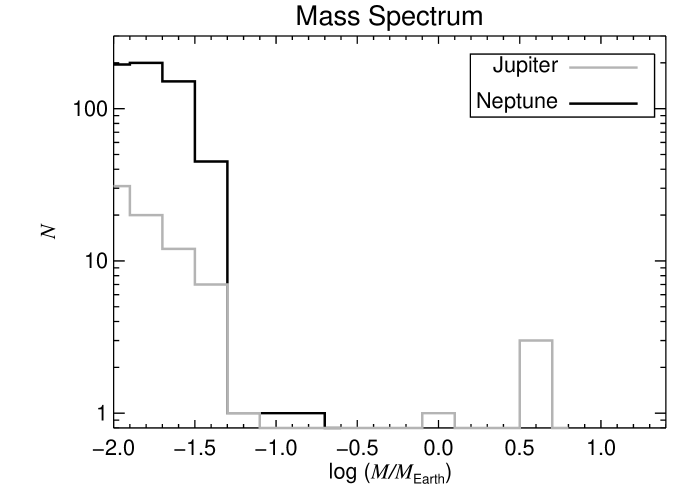
Figure 10: Mass spectrum at the end of the Jupiter (Sect. 5) and Neptune (Sect. 6) simulations. The most massive planet in the Neptune case is the Trojan of 0.16  $M_{\oplus}$. It is followed by another Trojan of 0.09 $M_{\oplus}$. In the Jupiter case the most massive planets are formed within the vortices at the outer edge of the gas gap. It includes the three super-Earths and a 8 $M_{\rm Mars}$ planet. The Jupiter simulation was terminated at 83 orbits. At that time, the mass in the tadpole orbits was split into 19 lunar-sized objects in the mass range 1-5 $M_{\rm Moon}$. Other 26 gravitationally bound objects of mass between 0.5 and 1 $M_{\rm Moon}$ are also observed in the co-rotational region.

Fast rocky planet formation also occurs in the vortices the giant planets induce at the edges of the gas gaps they open. In this case, the 30 cm particles set the record of highest concentration, by collapsing into a super-Earth encerring as much as 17 Earth masses. The mass is likely to be overestimated, since the vortex captured virtually all of the influx of particles from the outer disk, but this result nonetheless illustrates that the efficiency of vortex trapping for particles this size is superb. For other particle radii, the mass spectrum shows that dozens of Mars-sized planets were formed, along with hundreds of Moon-sized objects.

We compare runs with single and multiple particle species, finding that gas drag modifies the streamlines in the tadpole region around the classical L4 and L5 points. As a result, particles of different species have their stable points shifted to different locations. This brings down the mass of the Trojan planets, as now the clumps are segregated spatially by size, each of them having less mass available for assemblage. As a result, collapse is hindered in a low-resolution run with 256² grid points and $10^{5}$ particles equally distributed in mass and number among four species (1, 10, 30, and 100 cm). Counter-intuitively, a run with the same parameters but without self-gravity achieved higher mass concentrations (up to 6 $M_{\oplus}$). We conclude that the gravity of the solids modifies the stability of the tadpole orbits. Inside the massive vortices, the tidal forces from the gas also stall the gravitational growth of the solids into planets. The same negative results are observed when the number of numerical super-particles is raised by a factor 4.

Collapse resumed when the grid resolution was refined by a factor 2, producing 3 super-Earth mass planets at the outer edge of the gap. The most massive one has 4.5 $M_{\oplus}$ by the end of the simulation. The other super-Earths are of 4.36 and 4.14  $M_{\oplus}$. In addition, a fourth, smaller, planet of 8.0 $M_{\rm Mars}$ was also formed within the gap edge vortices. These planets are composed primarily of 30 cm particles ( $\approx$50%), with smaller and almost equal shares of 10 cm and 1 m, and only trace amounts of 1 cm particles. Judging by their mass and location, these objects may be the embryos that gave rise to planet Saturn. Although the distance of formation of Saturn in this model seems too close to Jupiter, it is not at all unlikely that Saturn was indeed formed in this orbital position. The ice giants Uranus and Neptune are presently located in regions of the solar system where the dynamical timescales are too large and the densities are too low to account for their current masses (Thommes et al. 2002, and references therein). This is an indication that they were formed further in and, therefore, that the giant planets displayed a much more compact spacing in the early Solar system than they present today. Our results seem to corroborate this scenario

When the mass of the perturber is reduced to that of Neptune, the asymmetry between L4 and L5 is accentuated. The L5 point of the particles of $a_{\bullet}$=10 cm moves to $\approx$35^∘behind Neptune, and the $a_{\bullet}$=1 m to $\approx$25^∘. The L4 point was shifted too far ahead of the planet and eventually lost all particles, a behavior attributed to its merging with the shifted unstable L3 point (Peale 1993, Murray 1994). Of the particles retained at L5, the ones of 10 cm concentrated into a 1.6 $M_{\rm Mars}$ Trojan planet.

One question to ask is if the formation of Trojan bodies as massive as terrestrial planets is so easily achievable, why we do not see it in the Solar System. The answer might lie in the fact that, according to recent models by Morbidelli et al. (2005), all Trojan orbits of the Jovian system were de-stabilized when Jupiter and Saturn crossed the 2:1 mean motion resonance. The initial Trojan population of Jupiter was lost and a new one was captured. Without the gas to damp their motions and increase the number density, the new Trojan population could not assemble into rocky planets. This scenario raises the possibility that in extrasolar planetary systems with only one giant or with giants that did not undergo the destructive resonance crossing that Jupiter and Saturn underwent, Trojan Earth-mass companions to the giant planets are common. This includes the giants in Earth-like orbits in a list of potentially habitable stellar systems.

Of course, it might as well be that the formation scenario we present is overly simplistic and that some important piece of physics that prohibits the process is missing. We did not include, for instance, the possibility of destructive collisions between boulders. Checking the velocity dispersion at the bound clumps, we find that they are typically lower than 10 m s^-1for a formed planet. As the initial stages of collapse, however, the speeds are greater, 10-30 m s^-1, eventually reaching as fast as 80 m s^-1. These speeds are comparable to or larger than the break-up collisional speeds ($\sim$10 m s^-1, Benz 2000). These high collision speeds indicate that collisional fragmentation will play an important role during the gravitational collapse in a more realistic coagulation-fragmentation model (Brauer et al. 2008a). On the other hand, the fact that collapse occurs for particles of 1-10 cm radius is particularly relevant since they are too small to be easily destroyed by collisions. Moreover, the escape velocities of the formed clumps are high enough so that most debris of catastrophic collisions might remain bound. Johansen et al. (2008) find that cm-sized fragments of such collisions are easily swept up away from the midplane by turbulent motions. This leaking is anticipated to not occur in the cases presented in this paper, where planets are formed inside vortices. As vortices do not have vertical shear and revolve at the Keplerian orbital rate (Klahr & Bodenheimer 2006) the sedimenation of the solids layer does not trigger the Kelvin-Helmholtz instability (Johansen et al. 2006b) when this sedimentation happens inside a vortex. The sedimentation is therefore more efficient, which helps collapse.

Our neglecting of coagulation is also an issue that causes pause. Solid bodies grow by sweeping up smaller dust grains, so coagulation raises the possibility that the trapped rocks and boulders might breach the meter-size barrier inside the gap edge vortices and Lagrangian gas clouds. If so, they would produce km-sized bodies that are too loosely coupled to undergo gravitational collapse in the way presented in this paper. Brauer et al. (2008b) has indeed showed that growth to kilometer-size is highly favored within gas pressure maxima. However, the timescale for coagulation seems to be slow ($\sim$1000 yr) compared to the timescales we observe for gravitational collapse in all cases except for the formation of Trojan planets with the $a_{\bullet}$=1 cm particles. In this case, the timescales are comparable and we can expect coagulation to influence the growth. In particular, coagulation onto the 1 cm particles can aid on replenishing the population of 10 cm and 30 cm particles lost during the Neptune phase.

Once a cluster of particles collapses to form a single object, aerodynamical drag ceases to be the most important driver of particle dynamics. Instead the planet enters the regime of gravitational drag in which it interacts with its own gravitational wakes. Since we solve for both the particle gravity (that causes the wakes) and gas gravity (that makes the wakes backreact on the particles), our simulations in principle resolve this stage as well, although limited by the grid resolution. However, the drag influence of the planet on the gas is strongly exaggerated, since the influence of particles is always spread over the nearest three grid points in each direction. The friction time is also still that of the individual rocks, where as a solidified body of a few thousand kilometers in size should have a much longer friction time. A better treatment would thus be to replace the ensemble of particles by a single particle representing the planet. This would also allow a much longer integration time, and we plan to go this way to model the long term evolution of the planet system in a future project.

An immediate question to ask is how (or if) the collapse would occur in three dimensions. Johansen & Klahr (2005), Fromang & Papaloizou (2006) and Lyra et al. (2008a) show that the particles are stirred up by the hydromagnetic turbulence to form a layer of finite vertical thickness, maintained by turbulent diffusion. We performed a 3D simulation of planet-disk interaction in spherical coordinates, similar to those of Bate et al. (2003), Kley et al. (2005) and Edgar & Quillen (2008), but inviscid instead of viscous. The Lagrangian points of the planet do not change much in 3D, with the scale height being about the same as in the unperturbed disk case. Fromang et al. (2004) and Lodato (2008) calculate the effects of self-gravity in the vertical extent of the disk, showing that the thickness is reduced by the disk’s self-gravity. This flattening of the scale height in self-gravitating disks bring it closer to the 2D configuration.

Of course, we are only assessing this by simple estimates based on isolated bits of physics done by individual works. A definite answer to this question has to be addressed by a 3D simulation that combines these effects.

The collapse of the solids is triggered by the gravitational influence of a perturber, but more fundamentally due to the presence of long-lived, high-pressure regions: the vortices and the accumulation of gas in the Lagrangian points. As such, a giant is not necessary for the rapid formation of rocky planets. Paardekooper et al. (2008) show that passing binaries can stir the material in the disk. Such encounters usually last for long times, and therefore gravitational collapse of the boulders might happen in such case. Vortices similar to the ones presented in this paper, excited by a giant planet, are also expected at the border of the dead zone (Varnière & Tagger, 2006; Lyra et al. 2008b). Therefore, the accumulation into rocky planets shown to occurs inside the vortices induced by a giant planet should also happen inside these dead zone vortices. If so, this paper provides not only a plausible mechanism for the formation of Trojan planets and Saturn, but also of the very first planetary embryos that - in the core accretion scenario - gave rise to Jupiter.

- (1) Baines, M. J., Williams, I. P., Asebiomo, A. S. 1965, MNRAS, 130, 63
- (2) Balsara, D. S., Tilley, D. A., Rettig, T., & Brittain, S. A. 2008, arXiv0810.0246
- (3) Barge, P., Sommeria, J. 1995, A&A, 295, 1
- (4) Bate, M. R., Lubow, S. H., Ogilvie, G. I., Miller, K. A 2003, MNRAS, 341, 213
- (5) Beaugé, C., Sándor, Zs., Érdi, B., Süli, Á. 2007, A&A, 463, 359
- (6) Benz, W. 2000, SSRv, 92, 279
- (7) Binney, J. & Tremaine, S. 1987, Galactic Dynamics, Princeton Univ. Press, Princeton, NJ
- (8) Bracco, A., Chavanis, P.-H., Provenzale, A.,& Spiegel, E. A. 1999, Physics of Fluids, 11, 2280
- (9) Brauer, F., Dullemond, C.P., & Henning, Th. 2008a, A&A, 480, 859
- (10) Brauer, F., Henning, Th., & Dullemond, C.P. 2008b, A&A, 487, L1
- (11) Chavanis, P.-H. 2000, A&A, 356, 1089
- (12) Edgar, R. G., Quillen, A. C. 2008, MNRAS, 387, 387
- (13) Fouchet, L., Maddison, S. T., Gonzalez, J.-F., Murray, J. R. 2007, A&A, 474, 1037
- (14) Freeman, K. C. 1970, ApJ, 160, 811
- (15) Fromang, S., Balbus, S. A., Terquem, C., De Villiers, J.-P. 2004, ApJ, 616, 364
- (16) Fromang, S., Nelson, R. P. 2005, MNRAS, 364, 81
- (17) Fromang, S., Papaloizou, J. 2006, A&A, 452, 751
- (18) Goldreich, P., Ward, W. R. 1973, ApJ, 183, 1051
- (19) Haghighipour, N. & Boss, A. P. 2003, ApJ, 583, 996
- (20) Haugen, N.E.L., Brandenburg, A., & Mee, A.J. 2004, MNRAS, 353, 947
- (21) Hockney, R. W., Eastwood, J. W. 1981, Computer Simulation Using Particles, McGraw-Hill, New York
- (22) Johansen, A., & Klahr, H. 2005, ApJ, 634, 1353
- (23) Johansen, A., Klahr, H., Henning, Th. 2006a, ApJ, 636, 1121
- (24) Johansen, A., Henning, Th., Klahr, H. 2006b, ApJ, 643, 1219
- (25) Johansen, A., Oishi, J. S., Mac Low, M.-M., Klahr, H., Henning, Th., & Youdin, A. 2007, Nature, 448, 1022
- (26) Johansen, A., Brauer, F., Dullemond, C., Klahr, H., & Henning, Th. 2008, A&A, 486, 597
- (27) Johansen, A., Youdin, A. 2007, ApJ, 662, 627
- (28) Klahr, H., Bodenheimer, P. 2006, ApJ, 639, 432
- (29) Kley, W., D’Angelo, G., Henning, Th. 2001, ApJ, 547, 457
- (30) Kwok, S. 1975, ApJ, 198, 583
- (31) Li, H., Colgate, S. A., Wendroff, B., Liska, R. 2001, ApJ, 551, 874
- (32) Lodato, G. 2008, arXiv0801.3848
- (33) Lyra, W., Johansen, A., Klahr, H., & Piskunov, N. 2008a, A&A, 479, 883
- (34) Lyra, W., Johansen, A., Klahr, H., & Piskunov, N. 2008b, arXiv0807.2622
- (35) Morbidelli, A., Levison, H. F., Tsiganis, K., Gomes 2005, Nature, 435, 462
- (36) Murray, C. D. 1994, Icarus, 112, 465
- (37) Paardekooper, S.-J. 2007, A&A, 462, 355
- (38) Paardekooper 2006, PhDT
- (39) Paardekooper, S.-J., Mellema, G. 2004, A&A, 425, 9
- (40) Paardekooper, S.-J., Thébault, P., Mellema, G. 2008, MNRAS, tmp, 370
- (41) Peale, S. J. 1993, Icarus, 106, 308
- (42) Pollack, J. B., Hubickyj, O., Bodenheimer, P., Lissauer, J. J., Podolak, M., Greenzweig, Y. 1996, Icarus, 124, 62
- (43) Rice, W. K. M., Lodato, G., Pringle, J. E., Armitage, P. J., & Bonnell, I. A. 2004, MNRAS, 355, 543
- (44) Rice, W. K. M., Lodato, G., Pringle, J. E., Armitage, P. J., Bonnell, I. A. 2006, MNRAS, 372, 9
- (45) Safronov, V.S. 1969, QB, 981, 26
- (46) Shakura, N.I., & Sunyaev, R.A., 1973, A&A, 24, 37
- (47) Skorov, Y. V. & Rickman, H., 1999, Planet. Space. Sci., 935, 949
- (48) Toomre, A. 1963, ApJ, 138, 385
- (49) Thommes, E. W., Duncan, M. J., & Levison, H. F. 2002, AJ, 123, 2862
- (50) de Val-Borro, M., Artymowicz, P., D’Angelo, G., Peplinski, A. 2007, A&A, 471, 1043
- (51) de Val-Borro, M., Edgar, R.G., Artymowicz, P., Ciecielag, P., Cresswell, P., D’Angelo, G., Delgado-Donate, E.J., Dirksen, G., Fromang, S., Gawryszczak, A., Klahr, H., Kley, W., Lyra, W., Masset, F., Mellema, G., Nelson, R., Paardekooper, S.-J., Peplinski, A., Pierens, A., Plewa, T., Rice, K., Schäfer, C., & Speith, R. 2006, MNRAS
- (52) Varnière, P., & Tagger, M. 2006, A&A, 446, L13
- (53) Weidenschilling, S. J. 1977, MNRAS, 180, 5
- (54) Weidenschilling, S. J., Cuzzi, J. N. 1993, Protostars and Planets III, p1031
- (55) Woitke, P. & Helling, C., 2003, A&A, 399, 297
- (56) Youdin, A. N., Goodman, J. 2005, ApJ, 620, 459
- (57) Youdin, A. N., Johansen, A. 2007, ApJ, 662, 613