Disordered driven lattice gases with boundary reservoirs and Langmuir kinetics

Abstract

The asymmetric simple exclusion process with additional Langmuir kinetics, i.e. attachment and detachment in the bulk, is a paradigmatic model for intracellular transport. Here we study this model in the presence of randomly distributed inhomogeneities (’defects’). Using Monte Carlo simulations, we find a multitude of coexisting high- and low-density domains. The results are generic for one-dimensional driven diffusive systems with short-range interactions and can be understood in terms of a local extremal principle for the current profile. This principle is used to determine current profiles and phase diagrams as well as statistical properties of ensembles of defect samples.

I Introduction

Despite several recent investigations Tripathy and Barma (1997a, 1998b); Krug (2000); Jain and Barma (2003); Shaw et al. (2004); Enaud and Derrida (2004); Chou and Lakatos (2004a); Harris and Stinchcombe (2004); Lakatos et al. (2006); Barma (2006); Juhász et al. (2006); Dong et al. (2007); Foulaadvand et al. (2007); Greulich and Schadschneider (2008a, b); Grzeschik et al. (2008) the influence of sitewise disorder in driven lattice gases is not yet fully understood Stinchcombe (2002).

One focus of studies on the influence of disorder and inhomogeneities was the Asymmetric Simple Exclusion Process (ASEP), especially its totally asymmetric variant (TASEP). This process is not only believed to capture the essentials of driven diffusive systems, but its homogeneous version is exactly solvable Derrida et al. (1993); Schütz and Domany (1993); Blythe and Evans (2007). The exact solution allows to determine the steady state properties analytically without approximations. These results can then be used as reference system to study the influence of disorder, inhomogeneities etc.

Here we will study the competition between disorder, realized through randomly distributed hopping rates associated to the sites in the TASEP, and Langmuir kinetics, i.e. attachment and detachment processes in the bulk. This is not only of theoretical interest due to the challenges posed by a non-trivial current profile, but also of direct relevance for the description of intracellular transport. The model which we will study here has originally been proposed to describe motor-based transport along microtubules. Although the microtubules itself are homogeneous, the presence of microtubule-associated proteins (MAP) Lodish et al. (2003) can create inhomogeneities which influence the motion of the motors Goldsbury et al. (2006).

In comparison to the ASEP, the current profile in the presence of Langmuir kinetics is no longer constant. This requires a slightly different approach since now a ”local” point of view becomes necessary. Our main interest will be in the (local) transport capacity defined in Sec. II. This important observable is now also a local variable and is of direct relevance for biological applications.

This paper is organized as follows: In Sec. II we define the models that are considered here and review some relevant results. Sec. III reports results for current and density profiles obtained by computer simulations. In Sec. IV we develop a theoretical framework that helps us to understand the simulation results and the phase diagram. This theoretical approach is applied in Sec. V to compute the probability that a randomly chosen defect configuration exhibits phase separation. Finally, Sec. VI gives a summary and conclusions.

II Model and Definitions

We consider driven lattice gases with open boundary conditions and Langmuir kinetics (LK). To be more specific we focus on the TASEP which is believed to be a paradigmatic example for this class of dynamic processes. Here different extensions considering LK have been proposed, e.g. by including the diffusion of detached particles Lipowsky et al. (2001); Lipowsky and Klumpp (2005). We will focus on a less detailed model variant, the TASEP/LK Parmeggiani et al. (2003, 2004), which is a TASEP with additional particle creation and annihilation in the bulk. The TASEP is defined on a lattice of $L$ sites which are numbered from $j=1$ to $j=L$ beginning at the left. Each site can be occupied by at most one particle. The motion of the particles from left to right is defined by (local) transition rates between adjacent sites. The corresponding hopping rates $p_{j}$ describing the transitions of particles to their right neighbours are inhomogeneous. We will focus on a binary distribution with two possible values $p_{j}=p$ or $p_{j}=q$ at each site $j$ where $q<p$. Sites with transition rate $p_{j}=q$ will be referred to as defect sites, while a site with transition rate $p_{j}=p$ is called a non-defect site. In the following we will call a stretch of $l$ consecutive defect sites a bottleneck of size $l$.

The boundaries of the system are connected to reservoirs so that particles can enter at the left end ($j=1$) and leave at the right end ($j=L$). The (fixed) densities $\rho_{0}$ and $\rho_{L+1}$ of the reservoirs control the effective entry and exit rates, $\alpha:=\rho_{0}$ and $\beta:=1-\rho_{L+1}$, respectively.

Langmuir kinetics is realized by creation and annihalition of particles in the bulk. This can be interpreted as particle exchange with a bulk reservoir and corresponds to attachment and detachment processes in the biological context. The corresponding rates will be considered to be homogeneous, i.e. independent of the position, throughout this paper .

For large system size the investigation is usually simplified by performing a continuum limit. Since crucial properties, like the bottleneck lengths in a disordered system, might depend on the system size we have to specify this limit more carefully. We define a weak continuum limit where terms of ${\mathcal{O}}(1/L)$ are neglected while terms of ${\mathcal{O}}(1/\ln L)$ are kept, and a strong continuum limit where we even neglect terms of ${\mathcal{O}}(1/\ln L)$. In the following we restrict ourselves to systems where the local creation and annihilation rates $\omega_{a}$ and $\omega_{d}$ are rescaled with the system size, while the global rates $\Omega_{a}:=\omega_{a}\,L$ and $\Omega_{d}:=\omega_{d}\,L$ are kept constant. Hence $\Omega_{a}$ and $\Omega_{d}$ are system parameters while $\omega_{a}$ and $\omega_{d}$ are adjusted to the system size. In particular in the (weak and strong) continuum limit, the local rates vanish: $\omega_{a},\omega_{d}\to 0$ for $L\to\infty$.

In homogeneous regions of these systems there is a unique current-density relation (CDR) $J(\rho)$, usually called fundamental diagram in the context of traffic flow, that unambiguously gives the current for a given particle density $\rho=\langle\tau_{j}\rangle$ on any site Popkov et al. (2003), where $\tau_{j}=0,1$ is the occupation number of site $j$. The CDR of the TASEP has a single maximum. Later, when we will also consider more general driven lattice gases, we will always assume that their CDR also has a single maximum. The maximum is at the point $\rho_{M}$ and takes the value $J_{M}=J(\rho_{M})$. In this case for a given current $J$, two possible values for the density, the high density value $\rho_{H}(J)>\rho_{M}$ and the low density value $\rho_{L}(J)<\rho_{M}$ exist.

For these systems, the non-conservation of particles can be expressed by a source term in the equation of continuity of the stationary state :

$$J_{j}-J_{j-1}=s(\rho)\,$$ (1)

where $J_{j}$ is the current through the bond between sites $j$ and $j+1$. The attachment of particles is assumed to be inhibited by particles occupying sites, so we assume $s(\rho)$ to be a globally decreasing function. In fact one can construct models with attractive interactions where $s(\rho)$ is an increasing function. However, those systems might exhibit non-ergodic behaviour Rákos et al. (2003) that we do not consider here. Since $\omega_{a},\omega_{d}\to 0$ in the continuum limit, we also have $s(\rho)\to 0$ in this limit. Hence locally the current is almost constant for large systems and the CDR is the same as in the corresponding system without LK Popkov et al. (2003); Greulich (2006).

The time evolution per time interval $\Delta t$ of the TASEP/LK can be written in terms of transition rules:

For $1<j<L$:

$$\begin{array}[]{lll}\mbox{Hopping}:&10\to 01&\quad\mbox{with probability }p_{j}\Delta t\\ \mbox{Attachment}:&0\to 1&\quad\mbox{with probability }\omega_{a}\Delta t\\ \mbox{Detachment}:&1\to 0&\quad\mbox{with probability }\omega_{d}\Delta t\end{array}$$ (2)

for $j=1$:

$$\begin{array}[]{lll}\mbox{Hopping}:&10\to 01&\quad\mbox{with probability }p_{1}\Delta t\\ \mbox{Entry}:&0\to 1&\quad\mbox{with probability }\alpha\Delta t\\ \mbox{Detachment}:&1\to 0&\quad\mbox{with probability }\omega_{d}\Delta t\end{array}$$ (3)

and for $j=L$:

$$\begin{array}[]{lll}\mbox{Attachment}:&0\to 1&\quad\mbox{with probability }\omega_{a}\Delta t\\ \mbox{Exit}:&1\to 0&\quad\mbox{with probability }\beta\Delta t\end{array}$$ (4)

Other transitions are prohibited. Here “0” represents empty and “1” occupied sites. We can write the time evolution of the density $\rho_{j}=\langle\tau_{j}\rangle$ as

$$\frac{d\rho_{j}}{dt}(t) = p_{j-1}\langle\tau_{j-1}(t)(1-\tau_{j}(t))\rangle-p_{j}\langle\tau_{j}(t)(1-\tau_{j+1}(t))\rangle$$ (5)

$$+ \omega_{a}(1-\rho_{j}(t))-\omega_{d}\rho_{j}(t)$$

in the bulk and

$$\frac{d\rho_{1}}{dt}(t) = -p_{1}\langle\tau_{1}(t)(1-\tau_{2}(t))\rangle$$ (6)

$$+ \alpha(1-\rho_{1}(t))-\omega_{d}\rho_{1}(t)$$

$$\frac{d\rho_{L}}{dt}(t) = p_{L-1}\langle\tau_{L-1}(t)(1-\tau_{L}(t))\rangle$$ (7)

$$- \beta\rho_{L}(t)+\omega_{a}(1-\rho_{L}(t))$$

at the left and right boundary, respectively. The parameters $\alpha,\beta$ correspond to the generic boundary rates defined before. The source term is $s(\rho)=\omega_{a}(1-\rho)-\omega_{d}\rho$. We call the hopping rates $p_{j}$ which are site-dependent properties intrinsic parameters which in the following will be considered as fixed, $p=1$ and $q=0.6$, if not stated otherwise. In contrast to this we consider the explicit dependence of the system properties on the external parameters $\alpha,\,\beta,\,\Omega_{a}$ and $\Omega_{d}$. Other driven lattice gases of the class characterized above can be written in the same way, while the local parameters might depend on the states in the vicinity of the sites and additional correlations might occur. Nonetheless one can assume that the TASEP/LK is quite universal as a paradigmatic model Greulich (2006).

In this work we are especially interested in randomly distributed defect sites. Here the defect density $\phi$, which is the probability that a given site is a defect site, serves as an additional system parameter. Hence, transition rates are distributed as

$$p_{j}=\left\{\begin{array}[]{ll}q&\quad\mbox{with probability }\phi\\ p&\quad\mbox{with probability }1-\phi\end{array}\right.\,\,.$$ (8)

Defect distributions of this kind are called disordered . The properties of such systems are not fully determined by the defect density $\phi$, but also depend on the spatial distribution of the defects. Since these properties can vary from sample to sample even for fixed system parameters, an investigation of ensembles of systems (e.g. disorder average) rather than single samples is an issue of physical relevance.

In the following sections we will make use of the particle-hole-symmetry exhibited by the TASEP/LK which is invariant under the symmetry operation

$$1\longleftrightarrow 0,\,\,\,\alpha\longleftrightarrow\beta,\,\,\,j\longleftrightarrow L+1-j,\,\,\,\Omega_{a}\longleftrightarrow\Omega_{d}\,\,.$$ (9)

However, the particle-hole-symmetry is not essential for the generic behaviour, but it allows to reduce the parameter space that needs to be investigated.

The TASEP/LK with one defect site was already investigated numerically and analytically in Pierobon et al. (2006). Now we want to generalize these results to arbitrary defect samples. Therefor we introduce a local quantity, the transport capacity $J^{*}_{j}$, which is the site-dependent maximum current that can be achieved by tuning the external parameters $\alpha,\,\beta,\,\Omega_{a}$ and $\Omega_{d}$ in the continuum limit . This quantity will be discussed in detail in section  IV.

III Observations by Computer Simulations

In this section we summarize some properties of the system that can be observed with Monte Carlo simulations. Therefor we compare quantities of the inhomogeneous TASEP/LK with the homogeneous TASEP/LK and the TASEP with defects. For simulations we used random-sequential update with fast hopping probability $p=1$. If not specified else, we fix $q=0.6$ as slow hopping rate. The unit of time is just one timestep so that probabilities and rates have the same numerical value.

III.1 Few defects/vanishing fraction of defects

Before we consider finite defect densities $\phi>0$ we discuss systems with a fixed number of defects in the continuum limit ($\phi=0$). Figs. 1–3 display the dependence of the densities and the current on the position in the system.

Fig. 1 shows the density and current profiles of a TASEP/LK-system with five defects, a homogeneous TASEP/LK-system and a TASEP with five defects in the low density phase. The density profiles of inhomogeneous and homogeneous TASEP/LK-systems differ only in the occurrence of narrow density peaks at the defects, while globally the density profile is the same. The current profiles of the homogeneous and inhomogeneous system are identical. In contrast, the density profile of the TASEP with defects at the same sites shows density peaks as well, but the current profile (and the density profile far from the boundaries) is flat. This is due to particle conservation while the lateral influx of particles allows a spatial variation of the current profile in the TASEP/LK where particles are not conserved in the bulk.

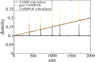
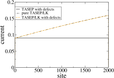
Figure 1: (Colour online) Comparison of current and density profiles for $\alpha=0.1$ and $\beta=0.9$ (low density phase) in the TASEP with defects, homogeneous TASEP/LK and TASEP/LK with defects and $\Omega_{a}=\Omega_{d}=0.1$.

Fig. 2 shows the corresponding situation for low exit rate and high entry rate. Due to particle-hole-symmetry, the results are analogous to the previous case. Adopting the terminology of the homogeneous system, the inhomogeneous TASEP/LK-system can be considered to be in a high and low density phase, respectively.

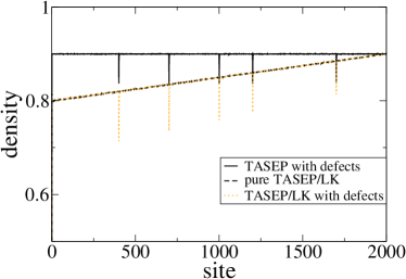
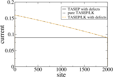
Figure 2: (Colour online) Comparison of current and density profiles for $\alpha=0.9$ and $\beta=0.1$ (high density phase) in the TASEP with defects, homogeneous TASEP/LK and TASEP/LK with defects.

Fig. 3 displays density profiles for $\alpha\approx\beta$. As in the case above, homogeneous and inhomogeneous TASEP/LK-systems exhibit the same density profiles, apart from the peaks. In this case we see a shock in the density profile which is characteristic for non-particle-conserving dynamics in the bulk and which cannot be observed in the particle conserving TASEP (except at $\alpha=\beta$).

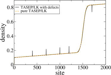
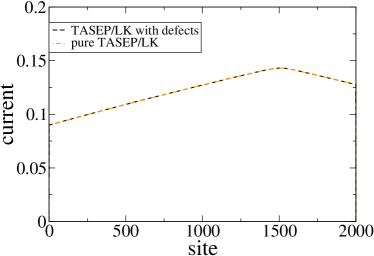
Figure 3: (Colour online) Comparison of current and density profiles for $\alpha=0.1$ and $\beta=0.15$ (high density phase) in the homogeneous TASEP/LK and TASEP/LK with defects.

Increasing the entry rate $\alpha$ for fixed and large $\beta$ one observes a queuing transition in Fig. 4: At a critical entry rate $\alpha^{*}$ the peak at the leftmost defect broadens, forming a high density region. This corresponds to phase separation and is also observed in the inhomogeneous TASEP at critical boundary rates. In the TASEP, however, the high density regime always extends to the left boundary. In contrast, the inhomogeneous TASEP/LK-system exhibits a stationary shock separating the low and high density region. Numerical finite-size scaling in Fig. 5 shows that the shock is getting sharper with increasing system size. Thus the high density region extends over a finite fraction of the system, corresponding to phase separation. In contrast, the peaks diminish for larger systems indicating that they are just local phenomena. We can associate this phase separation with a phase transition at the critical parameter value $\alpha^{\prime}$.

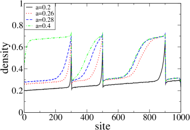
Figure 4: (Colour online) Density profiles for increasing values of $\alpha$ and fixed $\beta=0.9$. At a critical value $\alpha^{*}$ a high density region at the most right defect occurs (phase separation). For higher $\alpha$ multiple high density regions appear.

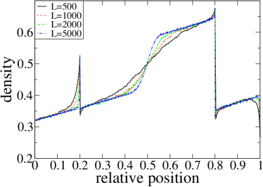
Figure 5: (Colour online) Density profiles for identical macroscopic parameters $\Omega_{a}=0.1,\,\,\Omega_{d}=0.1,\,\,\alpha=0.35,\,\,\beta=0.9$ but different system sizes $L$. The left boundary of the high density region (shock) becomes steeper with increasing system size, indicating a macroscopic regime.

Increasing $\alpha$ further moves the shock position to the left. The density profile right of the defect where phase separation occurred does not change anymore by varying the entry rate. The same is true for the output current at the right boundary $J_{\text{out}}=J(L)$. At some value of $\alpha$ a second high density region starts to form. Thus in a system with many defects multiple shocks can occur associated with alternating domains of high and low density.

Above a critical value $\alpha^{*}$, where a high density domain extends to the left boundary, the density profile and the current in the system is independent of the entry rate. Since this independence also holds for large $\beta$, we call this a Meissner phase in analogy to superconductors, where the magnetic field in the interior bulk is independent of exterior fields. This terminology was also used for the boundary independent phase in the homogeneous TASEP/LK Parmeggiani et al. (2004). However, one has to note that while in the homogeneous system there are long-range boundary layers in the density profile which do depend on boundary rates, the Meissner phase in the disordered system only exhibits short-range boundary layers. The current profile in fact does not depend on the boundary rates, both in the homogeneous and the inhomogeneous system.

Due to particle-hole-symmetry all considerations made in this section can be transferred to the high density phase by replacing $\alpha$ with $\beta$.

III.2 Finite fraction of defects and disordered systems

If the density of defects $\phi$ is finite and the number of defects is of order of the system size, even a local increase of the density in the vicinity of the defects has considerable impact on the average density due to the large number of defects. The effect can be observed in Fig. 6 where we have simulated disordered systems with small but finite defect density $\phi$ for small $\alpha$ and large $\beta$. In contrast to systems with few defects, the current profile of the disordered system differs from the that of the homogeneous system. This is due to the change of the density by defects, which leads to an altered influx of particles in the bulk by attachment/detachment. So the gradient of the current profile in the disordered system is different from the one in the homogeneous system and also from the system with few defects because in the latter the effect on the average density is negligible.

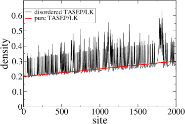
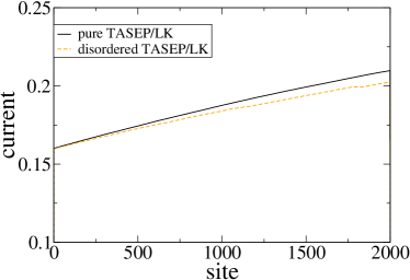
Figure 6: (Colour online) Comparison of current and density profiles for $\alpha=0.1$ and $\beta=0.9$ (low density phase) in the disordered TASEP/LK with defect density $\phi=0.1$ and homogeneous TASEP/LK.

Like in the TASEP/LK with few defects we observe multiple high and low density domains for large boundary rates, which is displayed in Fig.  7. In fact it is harder to distinguish macroscopic high and low density regimes in the disordered case because of the rapid changes of density on a microscopic scale. We have to simulate rather large systems in order to identify a macroscopic high(low) density domain by inspection. In Sec. V we introduce a numerical method that can detect high and low density domains automatically.

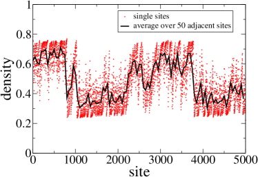
Figure 7: (Colour online) Density profile for $\alpha=0.9$ and $\beta=0.9$ in the disordered TASEP/LK with defect density $\phi=0.2$. One observes phase separation with alternating high and low density domains. The black line displays the density, averaged over 50 adjacent sites.

IV Theoretical treatment

In this section we develop a theoretical framework for the observations made by Monte Carlo simulations. We expect that concepts developed in this section are generic for a larger class of disordered driven lattice gases that have a single maximum in the current-density relation and weak induced effective interactions between defects. The restriction “weak interaction” is discussed in detail in Greulich and Schadschneider (2008b). In addition, we assume that the bulk influx term $S(\rho)$ is decreasing with increasing density.

First we summarize the properties that distinguish the inhomogeneous (disordered) TASEP/LK from the TASEP and homogeneous TASEP/LK, respectively.

1. In the TASEP/LK the particle number is not conserved in the bulk. Therefore generically the current profile is not flat and stationary shocks can occur in the bulk. For particle conserving systems these are not possible Popkov et al. (2003); Evans et al. (2003).

2. In the homogeneous TASEP, the current is restricted by the upper bound $J^{\rm max}_{\rm hom}=p(1-p)=0.25$ (for hopping rate $p=1$) due to the bulk exclusion. Already a single defect site with lower hopping rate $q<p$ reduces this maximum stationary current Janowsky and Lebowitz (1992). In Pierobon et al. (2006) it was shown that also in the TASEP/LK a single defect site $d$ restricts the current by a value $J^{*}_{d}:=J^{\rm max}_{d}<J^{\rm max}_{\rm hom}$ at this site, that cannot be exceeded by tuning external parameters. The quantity $J^{*}_{d}$ is exactly the local transport capacity defined in Sec. II. However, due to the spatially varying current, this effect is only local and the maximum value of the current $J^{\rm max}_{i}$ on sites $i$ far away from the defect can be larger than $J^{*}_{d}$. For completeness, we define $J^{*}_{i}=J^{\rm max}_{\rm hom}$ on non-defect sites $i$, so the transport capacity is peaked on a single site. If the current imposed by the boundary rates is larger than the transport capacity of a defect, phase separation occurs, exhibiting stationary shocks. In the inhomogeneous TASEP no stationary shocks can occur in the bulk, thus the high density regime always fills the whole system left of the current limiting defect.

3. In systems with only few defects the relation between the average density and the current at a given site is the same as in the homogeneous system. Thus current profiles are almost the same (as long as the maximum current is not exceeded). In disordered systems with a finite fraction of defects, however, the current-density relation is not the same as in the homogeneous system and depends on $q$ and the distribution of defects, since the large number of density peaks have influence on the source term $s(\rho)$ in (1) on a macroscopic scale. Therefore the current profiles differ from the homogeneous case.

In order to capture these properties, we follow the concept of Pierobon et al. (2006) by focusing on the current profiles $J(x)$.

IV.1 The influence of defects: additional initial conditions

Locally the current profiles are determined by the continuity equation (1). Introducing the continuous variable $x:=\frac{i-1}{L-1}$, which is the relative position in the system, one can write $J_{i-1}=J_{i}-\frac{1}{L}\frac{dJ}{dx}+{\cal O}(1/L^{2})$. In the stationary state the continuity equation (1) becomes

$$\frac{dJ}{dx}=S(\rho)+{\cal O}(1/L)$$ (10)

where the global source term $S(\rho)=L\,s(\rho)$ was introduced. In the TASEP/LK, for example, we have $S(\rho)=\Omega_{a}(1-\rho)-\Omega_{d}\rho$. In the continuum limit we neglect terms of $\mathcal{O}(1/L)$ so that (10) becomes an ordinary first order differential equation in the continuous variable $x$. The system, however, has at least two initial conditions (e.g. the boundary conditions in the homogeneous case), thus it is overdetermined. Each initial condition at a point $x_{0}$ is associated with one solution of the differential equation (10) $J_{x_{0}}(x)$ for the current and $\rho_{x_{0}}(x)$ for density, respectively. We call the mathematical solutions to single initial conditions $J_{x_{0}}(x)$ and $\rho_{x_{0}}(x)$ local current/density profiles. Physically these solutions are not necessarily realized.

For the TASEP/LK with a single defect it was shown by Pierobon et al. Pierobon et al. (2006) that the finite transport capacity at the defect site, corresponding to a local upper bound of the current, can be regarded as an additional condition on the current profile. They argued that the local solution of (10) with the initial condition $J(x_{d})=J^{*}(x_{d})$ becomes relevant if the local current profiles of the boundary conditions exceed $J^{*}$ at the defect site. Here we want to justify this approach and generalize it to a larger class of driven lattice gases with many defects, including randomly disordered systems, that meet the restrictions noted earlier in this section.

In Greulich and Schadschneider (2008b) it was shown that the maximum current in particle conserving driven lattice gases with randomly distributed defects but low defect density depends approximately only on the size of the longest bottleneck (Single Bottleneck Approximation, SBA). This fact, together with the observations made in Pierobon et al. (2006), motivates the generalization of the transport capacity to driven lattice gases (including TASEP/LK) with many defects but low defect density, introducing an approximation similiar to SBA. We call it the locally independent bottleneck approximation (LIBA): The transport capacity at a site $x$, $J^{*}(x)$, is approximately equal to the maximum current that can be achieved by tuning the boundary rates in the corresponding system containing only one bottleneck at this site . Thus $J^{*}(x)$ can be obtained by refering to a single-bottleneck system where all other defects (except the bottleneck at site $x$) have been removed.

In systems without LK the current is spatially constant and cannot exceed the minimum of $J^{*}(x)$ which corresponds to the transport capacity of the longest bottleneck, since in single bottleneck systems the maximum current is equal to the local transport capacity $J^{*}(x)$ and decreases with $l$ Greulich and Schadschneider (2008a); Dong et al. (2007); Chou and Lakatos (2004b). In this case the LIBA reduces to the SBA.

The LIBA neglects the influence of other defects on the transport capacity at site $x$. Nonetheless, we claim that the influence of other defects on the transport capacity can be considered as a perturbation in the same way as it is the case for the SBA in particle conserving systems Greulich and Schadschneider (2008a). Since the local attachment and detachment rates vanish in the continuum limit, the transport capacity of a bottleneck should be the same as in the corresponding particle conserving system. Therefore $J^{*}(x)$ is independent of $\Omega_{a}$ and $\Omega_{d}$. For the TASEP without LK analytical results are available Greulich and Schadschneider (2008a); Chou and Lakatos (2004b) that can be used to obtain approximations for the transport capacity. Since the maximal current in these systams depends only on the bottleneck length $l(x)$ Greulich and Schadschneider (2008a); Dong et al. (2007) this holds also for the transport capacity. The concept of a local transport capacity is applicable if interactions of defects near a bottleneck are not to large and distances of defects are not too small (i.e. low defect density ).

Hence, the transport capacity $J^{*}(x)$ yields an upper bound for the current profile,

$$J(x)\leq J^{*}(x)\hskip 14.22636pt\mbox{ for all $x$,}$$ (11)

while the function $J^{*}(x)$ of course is not continuous. Since on non-defect sites (which correspond to bottlenecks of size $l=0$) the transport capacity is $J^{*}=J^{\rm max}_{\rm hom}$, it is sufficient to check condition (11) for defect sites. Their number is finite in finite systems but can be infinite in the continuum limit (e.g. for disordered systems with finite defect density).

The problem of condition (11) is that it is given as an inequality and does not provide initial conditions for (10) on the defect sites. We now want to show that (11) is identically fullfilled by a set of initial conditions

$$J(x)=J^{*}(x)\hskip 14.22636pt\mbox{ at defect sites $x$}\,\,,$$ (12)

if one assumes additionally that the physical local solution at $x$ is selected by shock dynamics.

First of all, if we assume the conditions (12) we see that, in contrast to the boundary conditions of the system which are usually given by a fixed density, the initial condition imposed by a defect provides the possibility of two realizations of the local density profile. Given the initial condition $J(x_{0})=J^{*}(x_{0})$ at a point $x_{0}$, only the current is a fixed initial condition while, due to the non-unique inversion of the current-density relation (one maximum!), there are two possible values for the density, $\rho_{H}$ and $\rho_{L}$ (with $\rho_{H}>\rho_{L}$), leading to two possible local solutions of (10), a high density solution $J_{H}(x)$ and a low density solution $J_{L}(x)$:

$$J^{*}\begin{array}[]{l}\nearrow\\ \searrow\end{array}\begin{array}[]{l}\rho_{H}\longrightarrow J_{H}(x-x_{0},J^{*})\\ \\ \rho_{L}\longrightarrow J_{L}(x-x_{0},J^{*})\end{array}$$ (13)

Taking into account shock dynamics, a constraint on the selection of a physical solution is given by the collective velocity

$$v_{c}(x)=J^{\prime}(\rho(x))$$ (14)

where $J(\rho)$ is the current density relation and the prime denotes the derivative with respect to $\rho$ Kolomeisky et al. (1998). A solution can only propagate away from the initial point if the direction of $v_{c}$ is pointing away from it, i.e. left of it only solutions with $v_{c}<0$ can exist, while right of it solutions must have $v_{c}>0$. In a system with a single maximum at density $\rho_{m}$ in the CDR, $\frac{dJ}{d\rho}>0$ for $\rho<\rho_{m}$ and $\frac{dJ}{d\rho}<0$ for $\rho>\rho_{m}$, thus left of an initial point, only the high density solution $J_{H}$ can be realized, while right of it only $J_{L}$ can physically exist. This principle is displayed in Fig. 8, top. Hence, each initial condition at a point $x_{0}$ can have its own solutions. We denote these local solutions by

$$J(x-x_{0},J^{*})=\left\{\begin{array}[]{lc}J_{H}(x-x_{0},J^{*})&\mbox{for $x\leq x_{0}$}\\ J_{L}(x-x_{0},J^{*})&\mbox{for $x>x_{0}$}\end{array}\right.\,\,.$$ (15)

Actually the dependence on $J^{*}$ can easily be obtained by a shift operation if two functions $\tilde{J}_{L}(x)$ and $\tilde{J}_{H}(x)$ with initial conditions $\tilde{J}_{L}(0)=J^{0}_{L}$ and $\tilde{J}_{H}(0)=J^{0}_{H}$, where $J^{0}_{L}$ and $J^{0}_{H}$ are arbitrary chosen values in the high- and low density branch of the CDR. If the range in both branches of the CDR includes $J=0$, one can simply choose $J^{0}_{L}=J^{0}_{H}=0$ . Since the ODE (10) is of first order and does not explicitly depend on $x$, the high and low density solutions unambigiously depend on $\rho$ and are monotonic. Thus different local solutions $J_{L,H}$ can only differ by a shift in the variable $x$. An arbitrary solution $J_{L,H}(x-x_{0},J^{*})$ can be obtained by shifting $\tilde{J}_{L,H}(x)$ by an amount $\tilde{x}_{L,H}(J^{*})$ so that the value of the shifted function at $x=0$ is equal to $J^{*}$. The functions $\tilde{x}_{L,H}(J^{*})$ are just the inverse functions of the unique functions $\tilde{J}_{L,H}(x)$. Then the local solutions at a point with initial condition $J^{*}$ are given as

$$J(x-x_{0},J^{*})=\tilde{J}(x-x_{0}-\tilde{x}(J^{*}))\,.$$ (16)

The functions $\tilde{J}_{L,H}(x)$ and $\tilde{x}_{L,H}(J)$ can for example be obtained by numerical solution of (10) with initial conditions $J^{0}_{L,H}$.

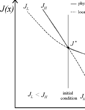
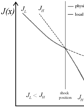
Figure 8: Top: Local solutions in the vicinity of a point with an initial condition $J^{*}$. Due to the non-unique inversion of the current-density relation, there are two possible solutions. Since for a physical solution the direction of the collective velocity must point away from this position, only solutions with maximal current are realized.
Bottom: Intersection point of local solutions of the density profile. The constraint that only upward shocks can exist implies that only solutions with minimal current are physically realized.

IV.2 Selection of the global current profile

The physically realized global current profile in the steady state is also determined by shock dynamics Popkov et al. (2003); Kolomeisky et al. (1998). Shocks manifest themselves as discontinuities in the density profiles. If they are stationary they connect different local steady state solutions of (10) to form a global solution. The crucial quantity for this selection is the shock velocity

$$v_{s}=\frac{J_{+}-J_{-}}{\rho_{+}-\rho_{-}}$$ (17)

that determines the propagation of a discontinuity in a (not necessarily stationary) density profile. Here $J_{+}$($\rho_{+}$) is the current (density) right of the shock and $J_{-}$ ($\rho_{-}$) is the current (density) left of the shock. In homogeneous driven lattice gases with a single maximum in the CDR only upward shocks with $\rho_{+}>\rho_{-}$ can exist (see for example Kolomeisky et al. (1998); Schütz (2001)). In Popkov et al. (2003) this was generalized to systems with particle creation and annihilation in the bulk, as long as the local creation and annihilation rates vanish in the continuum limit, i.e. $s(\rho)\to 0$ for $L\to\infty$. In this case, the CDR is the same as in the corresponding particle conserving system.

In inhomogeneous systems there can also be “downward” discontinuities at the defect sites due to the imposed maximum current. However, these discontinuities usually are not called “shocks” since their dynamics differ. In contrast to shocks they are sharp also in finite systems, thus there are no fluctuations. Due to the local character of $v_{s}$ and $v_{c}$ we can state that away from defects, where locally the system is homogeneous, only upward shocks can exist.

Since the source term $s(\rho)$ of (1) vanishes in the continuum limit, shocks can only be stationary at intersection points of a high and a low density solution $J_{H}(x)$ and $J_{L}(x)$. So only at these intersection points a switch of the physical realized local solution can occur. Note that local solutions of the same kind $J_{L}$ or $J_{H}$ cannot intersect since the differential equation (10) is of first order. Since $S(\rho)$, which determines the slope of the current profile, is assumed to be a monotonically decreasing function in $\rho$, we have $S(\rho_{H})<S(\rho_{L})$, hence the gradient of the high density solution $J_{H}(x)$ is smaller than the one of the low density solution $J_{L}(x)$. Therefore left of an intersection point, we have $J_{L}(x)<J_{H}(x)$, while right of it $J_{H}(x)<J_{L}(x)$. Since $J_{L}$ is the physical solution left of a shock and $J_{H}$ right of it, always the minimal local solution is the physical one (see Fig. 8, bottom). We define the minimal envelope of all the local current profiles as the capacity field of the system

$$\mathcal{C}(x):=\min_{x^{\prime}}\left\{J(x-x^{\prime},J^{*}(x^{\prime}))\right\}$$ (18)

with defects at the points $x^{\prime}$. This function does not depend on the boundary rates. The capacity field is a generalization of the capacity introduced in Pierobon et al. (2006). Note that in general the capacity field is not identical with the local transport capacity $J^{*}(x)$ . The local transport capacity can be viewed as the source or “charge” of the capacity field. In this view, the function $\tilde{J}_{L,H}(x-x_{0})$, which generates all local current profiles via (16), can be called the “Green’s function” of the capacity field.

Additional conditions on the current profile are given by the boundary rates so that $\rho(0)=\alpha$ and $\rho(1)=1-\beta$. Of course the maximum current of the homogeneous system $J^{\rm max}_{\rm hom}$ remains an upper bound also in the inhomogeneous system. The capacity field together with the boundary conditions can be used to express the physically realized current profile as

$$J(x)=\min\left[J_{\alpha}(x),J_{\beta}(x),\mathcal{C}(x)\right]$$ (19)

This principle is the generalization of the extremal current principle for the homogeneous TASEP Popkov and Schütz (1999). It provides a tool to obtain the global current profile if it is possible to obtain the local solutions of (10) and the local maximum current $J^{*}(x)$.

Indeed the global current profile given by (19) identically fulfills the condition (12) that the current must always be lower than the transport capacity.

In Fig. 9 we compare computer simulations of a system with a few defects with results obtained by the minimal principle (19) in order to illustrate some features of the TASEP/LK with defects. We chose high boundary rates, so that the resulting current profile is exactly the capacity field ${\mathcal{C}}(x)$. For the values $\Omega=\Omega_{a}=\Omega_{d}=0.2$ analytical results for the local current profiles in the continuum limit are available. Following Parmeggiani et al. (2003); Evans et al. (2003) we used the reference functions $\tilde{J}_{L}(x)=\Omega x-\Omega^{2}x^{2}$ and $\tilde{J}_{H}=-\Omega x+\Omega^{2}x^{2}$ that obey the initial condition $\tilde{J}_{L,H}(0)=0$ to reproduce the local solutions of (10). The transport capacity was obtained in LIBA by results of a TASEP with a single bottleneck. The first three bottlenecks are well separated by a large distance. Here we see that LIBA works quite well and the current profile is reproduced by the minimal principle quite accurately. We also find that at the position of bottleneck 2, the actual current is less than the transport capacity since the local solution of defect 1 is less than $J^{*}(x_{2})$ . For bottleneck 4 there are deviations to LIBA since bottleneck 5 which is quite close to bottleneck 4 (distance $=$ 6 sites) perturbs the transport capacity by further decreasing it. Nonetheless also in this region the minimal principle works if one takes the real transport capacity instead of LIBA.

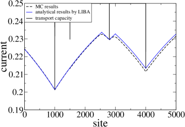
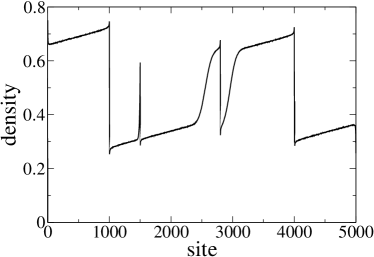
Figure 9: (Colour online) Comparison of MC results and semi-analytical results for the capacity field (= current profile for high boundary rates; here $\alpha=\beta=0.9$) by LIBA. Bottlenecks are at sites $x_{i}$ (first defect site) with size $l_{1}$:
$x_{1}=1000,\,\,l_{1}=4$
$x_{2}=1500,\,\,l_{2}=2$
$x_{3}=2800,\,\,l_{3}=2$
$x_{4}=4000,\,\,l_{4}=3$
$x_{5}=4008,\,\,l_{5}=1$.
Further details are given in the text.

IV.3 Local current profiles in the disordered TASEP/LK

We now want to quantify our results by finding the local solutions of the differential equation (10) and the continuity equation (1), respectively. For a numerical evaluation of these equations we need the CDR $J(\rho)$ and its inverse $\rho_{L,H}(J)$.

If there are only few defects in the system we have seen that the CDR is the same as in the homogeneous system, as long as the current is below the maximum current $J^{*}$, since the increase of the average density is negligible. Thus in the TASEP/LK with defects we can use the same CDR as in the homogeneous system: $J(\rho)=\rho(1-\rho)$. Therefore the local solutions are the same as the ones of the homogeneous systems.

The situation is different for a finite fraction of defects in the system. Then the average density is strongly influenced by the dense distribution of defect peaks which leads to an altered current-density relation even in the non-plateau region Barma (2006). We will give an approximation to calculate the current-density relation for small, but finite, defect density $\phi\ll 1$ if it is not too close to the maximum current. For that purpose we virtually divide the system into homogeneous subsystems with fast hopping rate $p$, while the slow hopping bonds connect these subsystems . In first instance we neglect correlations on the defect bonds. The subsystems have an average size ${1}/{\phi}$. In this point of view, the peaks at the defects are the boundary layers of the homogeneous subsystems. Without losing generality, we can assume the system to be in the low density phase and observe the local solution of the right boundary where peaks are concave. This can be transfered to high density solutions by particle-hole symmetry operation. Since $\omega_{a},\omega_{d}\sim 1/L$ we can neglect them for large systems when looking at a single subsystem, thus we can treat them as homogeneous TASEPs. In a large homogeneous TASEP in the low density phase, the density is given by $\rho_{0}=1/2-\sqrt{1/4-J}$ in the bulk far from the boundary. We can write the mass $m:=\sum_{i=1}^{L}\rho_{i}$ of the system as $m=L\rho_{0}+m_{p}$ with $m_{p}$ being the mass of the boundary layer. $m_{p}$ thus corresponds to the mass of a peak in the inhomogeneous system.

We approximate that the mass of the peaks does not depend on distance of adjacent defects. Then we can write the average density as

$$\rho(x)=\rho_{0}(J(x))+\phi\,m_{p}(J(x)),$$ (20)

since $\phi$ is the fraction of defect sites. Surprisingly this rather uncontrolled approximation is supported by Fig. 10 where we plotted the mass in a system with two defects in dependence on the distance of latter ones.

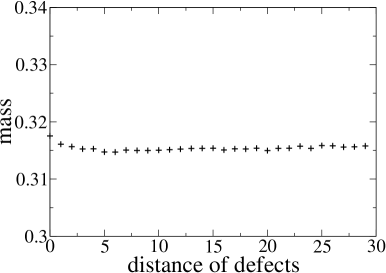
Figure 10: Mass $m$ of two density-peaks $m=\sum_{i=1}^{L}(\rho_{i}-\alpha)$ in the low density phase of the TASEP with two defects in dependence on the distance of the defects. One observes that the dependence is rather weak.

In this approximation, the mass of the peaks can be calculated analytically, since due to the independence of distance we can take it as the mass of the boundary layer in a large homogeneous TASEP, where exact results are available for given current $J$ Derrida et al. (1993). The density at a site $L-n$ is given by

$$\langle\tau_{L-n}\rangle=JS_{n}\left(J\right)+J^{n+1}R_{n}\left(1/(1-\rho)\right)$$ (21)

with

$$S_{n}(x) = \frac{1-\sqrt{1-4x}}{2x}-\sum_{j=n}^{\infty}\frac{(2j)!}{(j+1)!j!},$$ (22)

$$R_{n}(x) = \sum_{j=2}^{n+1}\frac{(j-1)(2n-j)!}{n!(n+1-j)!}x^{j}\,.$$ (23)

Thus the peak mass is

$$m_{p}=\sum_{n}\left[\langle\tau_{L-n}\rangle-\alpha(1-\alpha)\right]\,,$$ (24)

while the sum is truncated once the terms are small enough.

Eqs. (20)-(23) can be used to calculate the current $J$ for a given density $\rho$ in the low density phase (and in the high density phase by particle-hole symmetry) and vice versa:

$$J(\rho)=(\rho-\phi\,m_{p})(1-\rho+\phi\,m_{p})\,.$$ (25)

This relation can be used to obtain a local solution of the differential equation (10) for a given initial condition $J_{i}$ by iteration. In Fig. 11 we compared profiles obtained by this procedure with results from computer simulations. One observes an excellent agreement which holds if the current is not close to the transport capacity. Together with the minimal current principle (19) the global current profile can be obtained.

The corresponding density profile can be obtained by inverting the CDR with respect to its two branches. Regions with a high density solution of the current profile correspond to a high density domain with the density $\rho_{H}(J(x))$ obtained by the inverted current density relation. Analogous to that low density domains exist in regions of low density solutions.

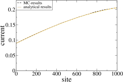
Figure 11: (Colour online) Comparison between simulation and analytical results for the current profile in a disordered system with $\phi=0.2,\,\omega_{a}=0.2,\,\omega_{d}=0.1$ for entry rate $\alpha=0.1$ and exit rate $\beta=0.9$. Since the current is less than the transport capacity throughout the system the profile corresponds to the local current profile of the boundary condition $\rho(0)=\alpha$. We observe excellent agreement between numerical and analytical results. This agreement holds for low current. Deviations occur only if the current comes close to the transport capacity.

IV.4 Phase diagram of disordered systems

We now want to investigate the phase diagram of inhomogeneous driven lattice gases.

If one of the local boundary solutions $J_{\alpha}(x)$ or $J_{\beta}(x)$ is the minimum of all local solutions in the whole system, we have a low density phase (L) in the former case and a high density phase (H) in latter one and there are no shocks in the system. These phases have the same macroscopic properties like in the corresponding homogeneous system.

If there are intersecting points of local solutions they manifest themselves as shocks in the density profile, separating high and low density regions (phase separation) corresponding to the realized high and low density solutions of the current profile. Phase separation can also be observed in homogeneous systems with Langmuir kinetics like the TASEP/LK and the NOSC-model Parmeggiani et al. (2003); Nishinari et al. (2005); Greulich et al. (2007). Here the local solutions of the boundaries $J_{\alpha}$ and $J_{\beta}$ can intersect leading to a single stationary shock in the density profiles, separating a low density domain left of it and a high density region right of it. This is called the shock phase (S) Parmeggiani et al. (2003) which is preserved as long as the minimum local profiles are the boundary current profiles. However, this kind of phase separation differs from the phase separation induced by defects. While in the S-phase the bulk behaviour is still determined by the boundary conditions, phase separation due to the finite transport capacity of defects is accompanied by a region where the current is “screened” by the defect(s) and is independent of the boundary condition, i.e. $\frac{\partial J(x)}{\partial\alpha}=0$ for all $x$ inside this region. If the phase separation is due to the screening by defects we rather refer to a defect-induced phase separated phase (DPS). If both boundary profiles $J_{\alpha}(x)$ and $J_{\beta}(x)$ are larger than $\mathcal{C}(x)$ in the whole system, the complete system is screened. The current profile is completely determined by the defect distribution and identical to the capacity field $\mathcal{C}(x)$. As argued in Sec. II we call this fully screened phase Meissner phase (M).

Another possible scenario is that the current near the boundaries is only limited by the maximum current of the bulk, i.e. ${\mathcal{C}}=J^{\rm max}_{\rm hom}$ and we have a maximum current phase with long ranging boundary layers like in the homogeneous TASEP. However in disordered systems with randomly disordered defects, distances of defects are microscopic and the probability that ${\mathcal{C}}=J^{max}_{\rm hom}$ vanishes in the continuum limit.

We can characterize the phases by two quantities:

1. The total length $\lambda_{H}$ of high density regions. This is the sum of individual high density regions and corresponds to the total jam length in traffic models Chowdhury et al. (2000).

2. The screening length $\xi$ , which is the size of the area where the current profile does not depend on the boundary conditions. This is exactly the region where the boundary independent capacity field $\mathcal{C}(x)<J_{\alpha,\beta}(x)$ and the local boundary profiles are not the physically realized ones.

In table 1 the behaviour of these quantities in the different phases is displayed. Indeed this can be used to define the phases. For $\xi=0$ defects do not influence the current profile and the system is in one of the “pure” phases, L,H or S, determined by the boundary conditions. If $0<\xi<1$ there is phase separation and a part of the system does not depend on the boundary conditions, the system is in the DPS-phase. For $\xi=1$ the complete system is screened and the current profile is solely determined by the defect distribution and the system is in the M-phase. The “pure” phases L,H,S can be characterized by $\xi=0$ and the vanishing of high density regions (L, $\lambda=0$), coexistence of high and low density regions (S, $0<\lambda<1$), and a global high density region (H, $\lambda=1$).

The transition from L or H to DPS is marked by a discontinuity in $\xi$, but it is continuous in $\lambda$. Indeed due to the discrete distribution of defects, $\xi$ itself is discontinuous throughout the DPS-phase while $\lambda$ is not. In the M-phase both $\xi$ and $\lambda$ are constant, while $\xi=1$ and $\lambda$ takes a finite value $\lambda_{M}$ that is determined by the fraction of high density regions in the capacity field $\mathcal{C}(x)$ which depends on the individual defect distribution.

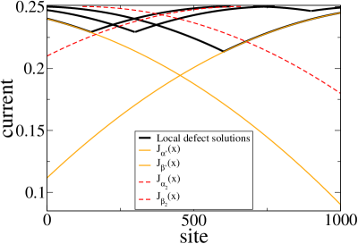
Figure 12: (Colour online) Illustration of some current profiles, including critical profiles. We see that the critical rates are related by the critical current profiles: $\alpha^{*}=\rho_{L}(J_{\beta^{\prime}}(1))$, while $\rho_{L}(\rho)$ is the inverted (low density) CDR and $J_{\beta^{\prime}}(1)$ is the local right boundary solution for $\beta=\beta^{\prime}$. An analog relation is valid for $\beta^{*}$. The bold lines are the local current profiles consistent with the initial conditions imposed by the defects, whose minimal envelope is the capacity field. The thin lines are the critical boundary profiles and the dashed line corresponds to phase separated boundary current profiles.

	L	H	S	DPS	M
$\lambda$	0	1	$\begin{array}[]{c}0<\lambda<1\\ \mbox{continuous}\end{array}$	$\begin{array}[]{c}0<\lambda<1\\ \mbox{continuous}\end{array}$	$\lambda_{M}$
$\xi$	0	0	0	$\begin{array}[]{c}0<\xi<1\\ \mbox{discontinuous}\end{array}$	1

Table 1: Values and properties of the characteristic order parameters $\xi$ and $\lambda$ in the different phases. These properties can be used to define phases.

We see that at most phase boundaries both quantities $\xi$ and $\lambda$ are non-analytic. At the transition from S to DPS though $\lambda$ is analytic, thus it cannot be characterized by $\lambda$. Hence for theoretical investigations it appears to be more convenient to use $\xi$ to discriminate defect- and non-defect phases. In simulations it is easier to detect phase separation (see next section) and use the non-analytic behaviour of $\lambda$ to obtain critical points. Due to the analytic behaviour between S- and DPS-phase, however, this approach is only applicable at L-DPS and H-DPS-transitions. The S-DPS transition has to be obtained by theoretical considerations.

In particle-conserving systems with defects the DPS- and S-phases vanish since no stationary shocks are possible. Here both $\xi$ and $\lambda$ are discontinuous at the transition to the M-phase. However, in these systems the Meissner phase usually is also called “phase separated phase” Greulich and Schadschneider (2008a) since no distinction between several phases with phase separation has to be made.

A sketch of the $\alpha-\beta$ phase diagram of a disordered driven lattice gas with LK is displayed in Fig. 13. Attachment and detachment rates are fixed, while here $\omega_{d}>\omega_{a}$. L-,H- and even S-phase might vanish for large $\Omega_{a,d}$ if $J_{\alpha=0}(L)>J^{*}(x_{b})$ at some point $x_{d}$ for any boundary rate $\alpha$ or $\beta$ so that phase separation with screening already occurs for vanishing boundary density. The dashed lines mark the phases of the homogeneous system. These pure phases are overlayed by the DPS- and M- phase which are characterized by the critical boundary rates $\alpha^{\prime},\beta^{\prime}$ and $\alpha^{*},\,\beta^{*}$. $\alpha^{\prime}$ and $\beta^{\prime}$ mark the minimal boundary rates at which the respective local boundary profile intersects the capacity field, i.e $J_{\alpha,\beta}>\mathcal{C}(x)$ for at least one point $x$, while at the rates $\alpha^{*},\,\beta^{*}$, $J_{\alpha,\beta}>\mathcal{C}$ everywhere, so that local boundary profiles cannot propagate into the bulk. In Fig. 12 we sketched some critical current profiles to illustrate the critical parameters. In parameter regions where $J_{\alpha}$ and $J_{\beta}$ do not intersect, $\alpha^{\prime}$ and $\beta^{\prime}$ do not depend on each other as well as $\alpha^{*}$ and $\beta^{*}$, hence the phase diagram has a simple structure with phase boundaries parallel to the parameter axes. Though, as we can see in Fig. 12, $\alpha^{\prime}$ and $\beta^{*}$ do depend on each other since $J(\beta^{*})=J_{\alpha^{\prime}}(1)$. The same relation is valid for $\beta^{\prime}$ and $\alpha^{*}$. Inside the region of intersecting boundary profiles (the shock phase of the homogeneous system), the structure is nontrivial. The phase transition betweeen S- and DPS-phase depends explicitely on the variation of the intersection points of boundary profiles and minimal defect profiles. Explicitely it is given by the condition that a triple points $x_{t}$ with $J_{\alpha}(x_{t})=J_{\beta}(x_{t})=\mathcal{C}(x)$ exist. One special case for which this condition can be solved exactly is the disordered TASEP/LK for $\Omega_{a}=\Omega_{d}$ in the strong continuum limit, where terms of ${\mathcal{O}}(1/\ln L)$ are neglected and the defect density $\phi$ scaling to zero as $\phi\sim 1/\ln L$. In this case the capacity field ${\mathcal{C}}$ is constant and the transition line is just a diagonal straight line. The phase diagram in the strong continuum limit is derived in the Appendix and displayed in Fig. 14. Though this limit is not quite physical it can be used as a reference point to argue that for finite defect densities the S-phase is convex (see also the Appendix).

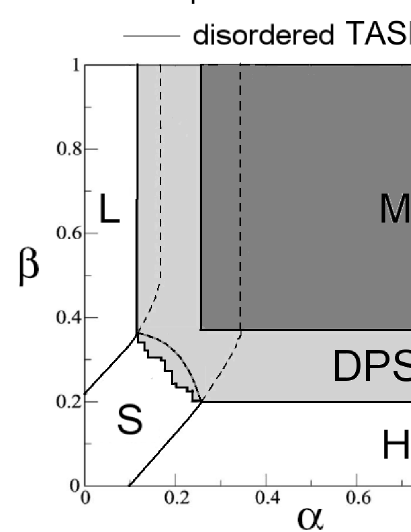
Figure 13: Phase diagram of the disordered TASEP/LK for $\Omega_{a}>\Omega_{d}$. The critical rates depend on each other as $\alpha^{*}=\rho_{L}(J_{\beta}^{\prime}(1))$, which is argued in the text. The transition line between S- and DPS-phase is not smooth in the weak continuum limit due to the unsmooth structure of the capacity field (bold line). In the strong continuum limit the DPS phase is concave (bold dashed line). The topology of other disordered driven lattice gases is expected to be the same.

If we go away from the strong continuum limit, $\mathcal{C}(x)$ is not a constant. The structure of $\mathcal{C}$ is not smooth as was argued in Sec. IV.2, so is the transition line. In Fig. 13 we displayed a rather generic sketch of a phase diagram that incorporates these arguments. Phase diagrams of other driven lattice gases with the properties noted in the introduction will have the same topology.

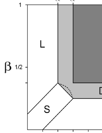
Figure 14: Phase diagram of the disordered TASEP/LK with $\Omega_{a}=\Omega_{d}=:\Omega$ in the strong continuum limit. The bold line at the S-DPS-boundary is valid for $\phi$ scaling as $1/\ln L$ and dashed line (sketched) is valid for finite defect density. The critical rates are given by $\alpha^{*}=\beta^{*}=(1-\sqrt{1-q})/2$, $\alpha^{\prime}=\alpha^{*}-\Omega$, same for $\beta$, with $\Omega=0.1,\,\,q=15/16$. The phase boundaries of the S-phase are of second order. For $\Omega>1/2$, L- and H-phase vanish.

V Expectation values for phase transitions

Like in particle conserving systems, the properties of disordered driven lattice gases with Langmuir kinetics depend strongly on microscopic details of the defect sample. Since we are interested in macroscopic properties that do not depend on microscopic defect distributions, we concentrate on probabilistic quantities of ensembles of systems. One quantity of interest is the expected fraction of systems that exhibit phase separation in an ensemble of systems with identical system parameters and defect density. In this section we derive a procedure to calculate this quantity based on analytical results obtained by the principles from the last section.

In order to compare these results with Monte Carlo simulations we introduce virtual particles similiar to second class particles Boldrighini et al. (1989) that indicate if phase separation occurs in the simulated system. These particles do not change the dynamics of the system. The predicted probability for phase separation is then compared with the relative frequency of phase separation in a set of simulations.

V.1 Automated detection of phase separation

We introduce so-called virtual particles (V-particles) to identify and distinguish high and low density regions. These particles do not follow the exclusion constraint, instead they can occupy all sites even if these are occupied by particles. The dynamics of the V-particles is the following: At the beginning, a V-particles is put on each defect site. After each lattice update the V-particles are updated sequentially beginning at the left. Each V-particle hops to the right if there is a particle on its site, while it hops to its left adjacent site if it is residing on an empty site. The V-particle cannot hop over slow bonds, thus if it is on a defect site, it cannot hop to the right, while if it is on a site right of a defect site, it cannot hop to the left. Hence, at any time, there is exactly one V-particle between each pair of contiguous defect sites. If the average density between two defects is larger than $1/2$, the V-particle tends to move to the right, while for $\rho<1/2$ it tends to move to the left. Thus, we can identify a high density region by a V-particle that is, on average, closer to the right defect. By computing the average distance of a V-particle to the defect right of it we can identify if there is a high density region in its vicinity.

Using this procedure we can run a large number of simulations and automatically identify whether high and low density regions coexist. In this way the relative frequency of phase separated systems and an estimate for the probability of phase separation can be determined.

V.2 Analytical approach for phase separation probability

We use the results from the last sections in order to derive a analytical approach that allows the determination of the probability that for a given defect density $\phi$ phase separation occurs. Again we consider ensembles of systems instead of a fixed configuration of defects.

The condition that no phase separation occurs is

$$J_{\alpha}(x)<J^{*}(x_{b})\mbox{\ \ and\ \ }J_{\beta}(x)<J^{*}(x_{b})\quad\mbox{for all $x_{b}$}.$$ (26)

The fact that only low density solutions can intersect high density solutions also implies that an increases of $\alpha$ leads to a left shift of phase boundaries (in the phase separated phase) to the left while a increase of $\beta$ moves the phase boundaries to the right. This can be seen in Fig. 4.

Following the LIBA we assume that the transport capacity at a position $x$ approximately depends only on the length of the bottleneck at this point, thus $J^{*}(x)\approx J^{*}(l(x))$. In a system with binary disorder there are on average $L(1-\phi)$ bottlenecks and the probability that one specific bottleneck has length $l$ is $P(l)=(1-\phi)\phi^{l}$ Greulich and Schadschneider (2008b).

The relation between bottleneck length and transport capacity $J^{*}(l)$ as well as its inverse relation $l(J^{*})$ can be obtained by analytical considerations or numerical computations in single bottleneck systems. The probability that the current is below the transport capacity at a given position $x$ is then

$$P(J<J^{*})=P(l<l(J))=\sum_{l^{\prime}=0}^{\lfloor l(J)\rfloor}P(l)=1-\phi^{\lfloor l(J(x))\rfloor}\,\,\,.$$ (27)

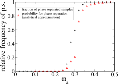
Figure 15: (Colour online) Fraction of samples that exhibit phase separation in dependence of the attachment rate $\omega_{a}$ for fixed $\alpha=0.1,\,\beta=0.9,\,\omega_{d}=0.3$. The system size is $L=1000$ and each data point is obtained by simulating 200 random defect samples with same system parameters. This is compared with analytical results obtained by (28).

.

The probability $\mathcal{P}$ that no phase separation occurs is equal to the probability that the current is below the transport capacity everywhere in the system:

$${\mathcal{P}}=\prod_{i=1}^{\langle N_{bn}\rangle}P(J(i)<J^{*}(l(i))=\prod_{i=1}^{L}(1-\phi^{\lfloor l(J(i))\rfloor})\,\,.$$ (28)

Here $N_{bn}$ is the number of bottlenecks from left to right, so $J(i)$ is the current at bottleneck $i$ counted from the left. Since on average there are $\langle N_{bn}\rangle=L(1-\phi)$ bottlenecks, we can determine $J(i)$ recursively by rescaling eq. (1) by the factor $1/(1-\phi)$ to obtain

$$J(i+1) = J(i)+\omega_{a}(1-\phi)(1-\rho(i))-\omega_{d}(1-\phi)\rho(i)\,,$$

$$\rho(i) = \rho_{0}(J(i))+\phi m_{p}\,\,.$$ (29)

This way the probability for phase separation, which explicitely depends on the system size can be computed iteratively by (28), while analytical results for $J(l)$ in the TASEP with a single bottleneck are available Greulich and Schadschneider (2008a). In comparison to Monte Carlo simulations, this computation can be made with little effort. In Fig. 15 we simulated ensembles of random defect samples for different parameter values. The fraction of samples exhibiting phase separation is determined by the method from subsection V.1 and compared with results obtained by (28). One observes a region with a quite steep increase of the probability. The analytical results fit the simulation results quite nicely, although there is a small shift to larger values of $\omega_{a}$.

VI Summary and conclusions

In this paper we have investigated the interplay between Langmuir kinetics (particle creation and annihilation in the bulk) and disorder, realized through randomly distributed hopping rates, in driven lattice gases connected to boundary reservoirs. Although both features provide a mechanism for phase separation (shock formation), the underlying mechanisms and dynamics is different and might lead to a form of competition.

Based on Monte Carlo simulations of the disordered TASEP/LK, a TASEP with Langmuir kinetics and site-disordered hopping rates, the main properties of such systems have been identified. Like in the disordered TASEP we observe narrow peaks in the vicinity of defect sites. Their width however vanishes in the continuum limit. For larger values of the boundary rates we observe defect-induced phase separation, where multiple macroscopic high and low density regions with a multitude of shocks occur.

These findings can be understood in terms of an extremal principle. In contrast to the principle originally proposed for homogeneous systems Popkov and Schütz (1999); Kolomeisky et al. (1998) it is a local principle for the current profile. This is a direct consequence of the interplay between Langmuir kinetics, which induces a site-dependence of the stationary current, and the randomly distributed inhomogeneities. In our approach we assumed that defects locally induce a reduced transport capacity imposing an upper bound to the current. For weakly interacting systems this quantity approximately depends only on the local distribution of defects, especially on the size of the bottleneck. In this approximation (LIBA) we can obtain the transport capacity by refering to single bottleneck systems. The transport capacity provides additional initial conditions to the differential equation (10) that gives the slope of the local current profile in the continuum limit, each of them representing a individual local solution. Shock dynamics impose additional conditions on the physical current profile. Hence, out of the multitude of solutions only the profile that locally minimizes all solutions is physically realized. The full current profile can be obtained by superposing the solutions of all single bottlenecks which are described in terms of the same “Green’s function” $\tilde{J}_{L,H}(x)$ defined in Sec. IV.2.

While in systems with only few defects local current profiles are almost identical to those of the homogeneous systems, they significantly differ in large systems with a finite fraction of defect sites. In the case of the disordered TASEP/LK local density profiles can be accurately reproduced by identifying the density peaks with boundary layers of small virtual subsystems where exact results are available.

The minimal principle can be used to predict some features of the phase diagram. As was already observed for single defects in Pierobon et al. (2006), defects can generate screened regions where the influence of boundary conditions vanishes. We can distinguish the original non-screened phases which are also present in homogeneous systems, a partially screened phase exhibiting phase separation and a fully screened phase where the influence of the boundary conditions vanishes completely. For the strong continuum limit where terms of ${\mathcal{O}}(1/\ln L)$ do not contribute, the minimal principle even allows the determination of the exact phase diagram, while in for the weak continuum limit at least most qualitative aspects of the phase diagram remain accessible.

The LIBA and the minimal principle can also be applied together with a statistical approach to obtain an approximation for the probability that a randomly produced disorder sample exhibits phase separation.

Although the results have been derived and tested on the TASEP/LK we believe that are generic for a large class of driven lattice gases, at least if they are ergodic with short-ranged interactions and a single maximum in the current-density relation. In more general processes the lateral current $s(\rho)$ takes the role of attachment/detachment processes.

APPENDIX: Phase transition lines in the strong continuum limit

Usually it is quite difficult to determine the transition line between S- and DPS-phase. One special case where it is possible to solve that problem exactly is in the strong continuum limit in the disordered TASEP/LK for $\Omega_{a}=\Omega_{d}=:\Omega$. In addition the number of defects is infinite, while the defect density is scaled to zero as $\phi=\mathcal{O}(1/\ln L)$. The average length of the longest bottleneck in a system of size $L$ scales as $\ln L/\ln\phi$ Krug (2000); Greulich and Schadschneider (2008b), so in the strong continuum limit there has to be an infinitely large bottleneck with a local transport capacity $J^{*}_{M}=q/4$. Moreover, we can say that this is the case for any small interval of length $\varepsilon$ if $\varepsilon$ is scaling slower than $\sqrt{1/L}$, corresponding to $L\sqrt{1/L}=\sqrt{L}$ sites. The global capacity field therefore simply is the constant function $\mathcal{C}(x)=q/4$. Since the defect density vanishes, the CDR is the same as in the homogeneous system as was shown in the last sections numerically and analytically. The local boundary current and density profiles will therefore be the same as in the homogeneous system. Now the problem we have to solve is equivalent to finding the transition from S- to LMH-phase in the homogeneous TASEP/LK if the homogeneous maximum current $J^{*}=1/4$ is exchanged by $q/4$ Parmeggiani et al. (2003); Evans et al. (2003). In these works, the transition line was determined to be $\tilde{\beta}^{*}(\tilde{\alpha})=\rho_{L}(J^{*})-\Omega-\tilde{\alpha}$. Inserting $J^{*}=q/4$, we obtain for the transition line

$$\tilde{\beta}^{*}(\tilde{\alpha})=1/2-\sqrt{\frac{1-q}{4}}-\Omega-\tilde{\alpha}$$ (30)

which is just a shift of the phase transition line to the right by the term $\sqrt{(1-q)/4}$. The properties of the phases of course are different to the ones in the homogeneous system as we have argued before (especially the absence of long ranged boundary layers). The phase diagram is displayed in Fig. 14. We have to point out that in this limit, the transition is of second order, since $\xi$ is continuous.

Nonetheless the vanishing of $\phi$ in the continuum limit is not quite physical, so we try to obtain at least qualitative results for the S-DPS transition line for finite $\phi$. In sec. III.2 and IV.3 we have seen that a small but finite defect density $\phi>0$ leads to a flattening of the local density profiles due to a broadening of the density peaks, so that their slopes $\frac{\partial\rho_{L,H}}{\partial x}$, which are positive for $\Omega_{a}=\Omega_{d},\,\,\alpha<1/2,\,\beta<1/2$, are decreasing for higher current $J$.

Assume the system is on the transition line between S and DPS, i.e. a triple point $x_{t}$ with $J_{\alpha}(x_{t})=J_{\beta}(x_{t})=q/4$ exists. A shift of both $\rho_{\alpha}$ and $\rho_{\beta}$ by an infinitisemal amount $dx$ also shifts the triple point though it persists. In parameter space, this corresponds to a movement along the transition line, while the boundary values are changed by

$$d\alpha = \left.\frac{\partial\rho_{\alpha}}{\partial x}\right|_{x=0}dx\,\,\,\mbox{ and }\,\,\,d\beta=-\left.\frac{\partial\rho_{\beta}}{\partial x}\right|_{x=1}dx$$ (31)

$$\Rightarrow \frac{d\beta}{d\alpha}=-\frac{\left.\frac{\partial\rho_{\beta}}{\partial x}\right|_{x=1}}{\left.\frac{\partial\rho_{\alpha}}{\partial x}\right|_{x=0}}$$ (32)

using the relations $\alpha=\rho_{\alpha}(0)$ and $\beta=1-\rho_{\beta}(1)$. Since the boundary current $J_{\alpha,\beta}$ is monotonously increasing with $\alpha$ and $\beta$ for $\alpha,\beta<1/2$, the flattening of the density profiles leads to:

$$\mbox{For }\beta>\alpha:\left.\frac{\partial\rho_{\beta}}{\partial x}\right|_{x=1}<\left.\frac{\partial\rho_{\alpha}}{\partial x}\right|_{x=0} \Rightarrow \,\,\frac{d\beta}{d\alpha}>-1$$ (33)

$$\mbox{For }\alpha>\beta:\left.\frac{\partial\rho_{\beta}}{\partial x}\right|_{x=1}>\left.\frac{\partial\rho_{\alpha}}{\partial x}\right|_{x=0} \Rightarrow \,\,\frac{d\beta}{d\alpha}<-1$$ (34)

along the transition line. This corresponds to a concave distortion of the DPS-phase as displayed in Fig. 14.

References

- Tripathy and Barma (1997a) G. Tripathy and M. Barma, Phys. Rev. Lett. 78, 3039 (1997a).
- Tripathy and Barma (1998b) G. Tripathy and M. Barma, Phys. Rev. E 58, 1911 (1998b).
- Shaw et al. (2004) L. Shaw, A. Kolomeisky, and K. Lee, J. Phys. A 37, 2105 (2004).
- Chou and Lakatos (2004a) T. Chou and G. Lakatos, Phys. Rev. Lett. 93, 198101 (2004a).
- Lakatos et al. (2006) G. Lakatos, J. O’Brien, and T. Chou, J. Phys. A 39, 2253 (2006).
- Barma (2006) M. Barma, Physica A 372, 22 (2006).
- Juhász et al. (2006) R. Juhász, L. Santen, and F. Iglói, Phys. Rev. E 74, 061101 (2006).
- Dong et al. (2007) J. Dong, B. Schmittmann, and R. Zia, J. Stat. Phys. 128, 21 (2007).
- Foulaadvand et al. (2007) M. E. Foulaadvand, S. Chaaboki, and M. Saalehi, Phys. Rev. E 75, 011127 (2007).
- Greulich and Schadschneider (2008a) P. Greulich and A. Schadschneider, Physica A 387, 1972 (2008a).
- Greulich and Schadschneider (2008b) P. Greulich and A. Schadschneider, J. Stat. Mech. p. P04009 (2008b).
- Grzeschik et al. (2008) H. Grzeschik, R. Harris, and L. Santen, arXiv:0806.3845 (2008).
- Krug (2000) J. Krug, Braz. Jrl. Phys. 30, 97 (2000).
- Enaud and Derrida (2004) C. Enaud and B. Derrida, Europhys. Lett. 66, 83 (2004).
- Harris and Stinchcombe (2004) R. J. Harris and R. B. Stinchcombe, Phys. Rev. E 70, 016108 (2004).
- Jain and Barma (2003) K. Jain and M. Barma, Phys. Rev. Lett. 91, 135701 (2003).
- Stinchcombe (2002) R. Stinchcombe, J. Phys.: Condens. Matter 14, 1473 (2002).
- Derrida et al. (1993) B. Derrida, M. R. Evans, V. Hakim, and V. Pasquier, J. Phys. A 26, 1493 (1993).
- Schütz and Domany (1993) G. Schütz and E. Domany, J. Stat. Phys. 72, 277 (1993).
- Blythe and Evans (2007) R. Blythe and M. Evans, J. Phys. A 40, R333 (2007).
- Lodish et al. (2003) H. Lodish, A. Berk, P. Matsudaira, C. Kaiser, M. Krieger, M. Scott, S. Zipursky, and J. Darnell, Molecular Cell Biology (W.H. Freeman and Company, 2003).
- Goldsbury et al. (2006) C. Goldsbury, M.-M. Mocanu, E. Thies, C. Kaether, C. Haass, P. Keller, J. Biernat, E. Mandelkow, and E.-M. Mandelkow, Traffic 7, 1 (2006).
- Lipowsky et al. (2001) R. Lipowsky, S. Klumpp, and T.M. Nieuwenhuizen, Phys. Rev. Lett. 87, 108101 (2001).
- Lipowsky and Klumpp (2005) R. Lipowsky and S. Klumpp, Physica A 352, 53 (2005).
- Parmeggiani et al. (2003) A. Parmeggiani, T. Franosch, and E. Frey, Phys. Rev. Lett. 90, 086601 (2003).
- Parmeggiani et al. (2004) A. Parmeggiani, T. Franosch, and E. Frey, Phys. Rev. E 70, 046101 (2004).
- Popkov et al. (2003) V. Popkov, A. Rakos, R. D. Willmann, A. B. Kolomeisky, and G. M. Schütz, Phys. Rev. E 67, 066117 (2003).
- Rákos et al. (2003) A. Rákos, M. Paessens, and G. M. Schütz, Phys. Rev. Lett. 91, 238302 (2003).
- Greulich (2006) P. Greulich, Diploma thesis, Universität zu Köln (2006).
- Pierobon et al. (2006) P. Pierobon, M. Mobilia, R. Kouyos, and E. Frey, Phys. Rev. E 74, 031906 (2006).
- Evans et al. (2003) M. R. Evans, R. Juhasz, and L. Santen, Phys. Rev. E 68, 026117 (2003).
- Janowsky and Lebowitz (1992) S.A. Janowsky and J.L. Lebowitz, Phys. Rev. A 45, 618 (1992).
- Chou and Lakatos (2004b) T. Chou and G. Lakatos, Phys. Rev. Lett. 93, 198101 (2004b).
- Kolomeisky et al. (1998) A. Kolomeisky, G. Schütz, E. Kolomeisky, and J. Straley, J. Phys. A 31, 6911 (1998).
- Schütz (2001) G. Schütz, in Phase Transitions and Critical Phenomena, edited by C. Domb and J. Lebowitz (Academic Press, 2001), vol. 19.
- Popkov and Schütz (1999) V. Popkov and G. M. Schütz, Europhys. Lett. 48, 257 (1999).
- Greulich et al. (2007) P. Greulich, A. Garai, K. Nishinari, A. Schadschneider, and D. Chowdhury, Phys. Rev. E 75, 041905 (2007).
- Nishinari et al. (2005) K. Nishinari, Y. Okada, A. Schadschneider, and D. Chowdhury, Phys Rev Lett 95, 118101 (2005).
- Chowdhury et al. (2000) D. Chowdhury, L. Santen, and A. Schadschneider, Phys. Rep. 329, 199 (2000).
- Boldrighini et al. (1989) C. Boldrighini, G. Cosimi, S. Frigio, and M. G. Nunes, J. Stat. Phys. 55, 611 (1989).