A Monte Carlo study of the three-dimensional XY universality class: Universal amplitude ratios

Institut für Theoretische Physik, Universität Leipzig

Postfach 100 920, D-04009 Leipzig, Germany

e–mail:   Martin.Hasenbusch@itp.uni-leipzig.de

We simulate lattice models in the three-dimensional XY universality class in the low and the high temperature phase. This allows us to compute a number of universal amplitude ratios with unprecedented precision: $R_{\Upsilon}=0.411(2)$, $R_{B}=2.83(1)$, $R_{\xi}^{+}=0.3562(10)$ and $R_{\xi}^{-}=0.850(5)$. These results can be compared with those obtained from other theoretical methods, such as field theoretic methods or the high temperature series expansion and also with experimental results for the $\lambda$-transition of ⁴He. In addition to the XY model, we study the three-dimensional two-component $\phi^{4}$ model on the simple cubic lattice. The parameter of the $\phi^{4}$ model is chosen such that leading corrections to scaling are small.

Keywords: $\lambda$-transition, Amplitude ratios, Classical Monte Carlo simulation

1 Introduction

In the neighbourhood of a second order phase transition various quantities diverge, following power laws. E.g. in a magnetic system, the magnetic susceptibility behaves as

$$\chi\simeq C_{\pm}|t|^{-\gamma}\;,$$ (1)

where $\gamma$ is the critical exponent of the magnetic susceptibility, $C_{+},C_{-}$ are the amplitudes in the high and low temperature phase, respectively, and $t=(T-T_{c})/T_{c}$ is the reduced temperature. Critical exponents like $\gamma$ assume universal values; i.e. they assume exactly the same value for all systems within a given universality class. Following Wilson (see e.g.[1]), such a universality class is characterized by the dimension of the system, the range of the interaction and the symmetry of the order parameter. In addition to the critical exponents, amplitude ratios like $C_{+}/C_{-}$ are universal, while the value of $C_{+}$ or $C_{-}$ depends on the microscopic details of the model. For a review on amplitude ratios see ref. [2].

In the present work we compute, using data obtained from Monte Carlo simulations of lattice models, the numerical values of four such universal amplitude ratios for the universality class of the three dimensional XY model. The $\lambda$-transition of ⁴He is supposed to share this universality class. At temperatures below the transition, ⁴He becomes superfluid. The $\lambda$-transition owes its name to the fact that the specific heat plotted as a function of temperature resembles the Greek letter $\lambda$. The order parameter of the $\lambda$-transition in ⁴He is the phase of a wave function. Therefore it should share the XY universality class, which is characterized by the O(2), or equivalently U(1), symmetry of the order parameter. The study of the $\lambda$-transition provides by far the most precise experimental results for universal quantities like critical exponents and amplitude ratios. Thus this transition gives us a unique opportunity to test the ideas of the renormalization group and to benchmark theoretical methods. For a review and an outlook on future experiments in space-stations see ref. [5].

The present work is the completion of ref. [6], where we had computed the ratio $A_{+}/A_{-}$ of the amplitudes of the specific heat. Our results can be compared with those obtained by using other theoretical methods and, which may be even more important, experimental results obtained for the $\lambda$-transition of ⁴He.

The outline of our paper is the following: First we define the models and the observables that are measured. We briefly discuss the Monte Carlo algorithm that has been used for the simulation. Since the continuous $O(2)$-symmetry is spontaneously broken in the low temperature phase, there is a Goldstone boson. As a consequence, the thermodynamic limit is approached with corrections that decay as inverse powers of the linear lattice size. Therefore, extracting estimates for the thermodynamic limit from Monte Carlo data requires special care. To this end, we summarize the relevant results of chiral perturbation theory as discussed in refs. [7, 8, 9]. Then we present our numerical estimates of various observables in the low and high temperature phases. Next we compute the amplitude ratios from these observables. Finally we compare our results with those of other theoretical methods and experiments.

2 The models

We study the $\phi^{4}$ model on a simple cubic lattice with periodic boundary conditions in each of the directions. The classical Hamiltonian is given by

$$H_{\phi^{4}}=-\beta\sum_{<x,y>}\vec{\phi}_{x}\cdot\vec{\phi}_{y}+\sum_{x}\left[\vec{\phi}_{x}^{2}+\lambda(\vec{\phi}_{x}^{2}-1)^{2}\right]\;\;,$$ (2)

where the field variable $\vec{\phi}_{x}$ is a vector with two real components. $<x,y>$ denotes a pair of nearest neighbour sites. The sites of the lattice are labelled by $x=(x_{1},x_{2},x_{3})$ with $x_{i}\in\{1,2,...,L_{i}\}$. Throughout we consider lattices with $L_{1}=L_{2}=L_{3}=L$. Note that in our convention, following ref. [10], the inverse temperature $\beta$ is absorbed into the Hamiltonian but does not multiply its second term. The partition function is given by

$$Z_{\phi^{4}}=\prod_{x}\left[\int\mbox{d}\phi_{x}^{(1)}\int\mbox{d}\phi_{x}^{(2)}\right]\;\;\exp(-H_{\phi^{4}})\;\;.$$ (3)

The reduced free energy density is then given by $f=-\frac{1}{L^{3}}\log(Z)$.

In the limit $\lambda\rightarrow\infty$ the classical XY (plane rotator) model is recovered. It is defined by the classical Hamiltonian

$$H_{XY}=-\beta\sum_{<x,y>}\vec{s}_{x}\vec{s}_{y}\;\;,$$ (4)

where $\vec{s}_{x}$ is a unit-vector with two real components. For $\lambda=0$ one gets the exactly solvable Gaussian model. For $0<\lambda\leq\infty$ the $\phi^{4}$ model undergoes a second order phase transition in the XY universality class; see e.g. ref. [11].

Power laws like eq. (1) are subject to corrections; see e.g. ref. [23];

$$\chi=C_{\pm}|t|^{-\gamma}\;\left(1+b_{\pm}t^{\theta}+...\right)$$ (5)

with $\theta\approx 0.5$ for the three-dimensional XY universality class. Such corrections complicate the determination of universal quantities from Monte Carlo simulations or high temperature series expansions of lattice models. Correction to scaling amplitudes like $b_{\pm}$ depend on the parameter $\lambda$ of the $\phi^{4}$ model. It is a rather old idea [12] to search for the value of such a parameter, where the leading correction to scaling amplitude vanishes. Note that the renormalization group predicts that the zero of the leading correction amplitude is the same for all quantities. It has been demonstrated numerically [13, 14] that such an improved value $\lambda^{*}$ indeed exists. The most accurate determination of the improved value is $\lambda^{*}=2.15(5)$ [10]. Previous estimates are $\lambda^{*}=2.07(5)$ in ref. [14] and $\lambda^{*}=2.10(6)$ in ref. [13].

We performed simulations at $\lambda=2.1$ and $\lambda=2.2$, where leading corrections to scaling are small. Following ref. [10] leading corrections to scaling at $\lambda=2.1$ and $\lambda=2.2$ should be at least by a factor of 20 smaller than in the XY model. Comparing results obtained with $\lambda=2.1$ and $\lambda=2.2$ allows us to estimate the effect of these small corrections. In ref. [10] the estimates $\beta_{c}=0.5091503(3)[3]$ and $\beta_{c}=0.5083355(3)[4]$ for the inverse critical temperatures at $\lambda=2.1$ and $\lambda=2.2$, respectively, were obtained. The number quoted in $()$ gives the statistical error, while the number given in $[]$ gives the systematic one. In the following analysis of our data we will just add up these two numbers. In order to clearly see effects due to leading corrections to scaling, we also have simulated the XY model. Recent estimates for the inverse of the critical temperature are $\beta_{c}=0.454165(4)$, $0.454167(4)$, $0.4541659(10)$ and $0.4541652(11)$ in refs. [15, 16, 17, 10], respectively. In the analysis of our numerical data we shall assume $\beta_{c}=0.0.4541655(10)$, which is roughly the average of the estimate of refs. [17] and [10].

2.1 Simulation algorithm

We have simulated the XY model using the single cluster algorithm [18]. The $\phi^{4}$ model was simulated using a hybrid of the single cluster algorithm and a local Metropolis algorithm. The cluster algorithm allows only to change the angle of the field $\vec{\phi}$. In order to to change the modulus $|\vec{\phi}|$, Metropolis updates are performed. Such a hybrid approach was originally proposed by Tamayo and Brower [19] for the one component $\phi^{4}$ model. The generalization to $N$ components is discussed in ref. [13]. For details of our implementation, in particular of the local updates see ref. [10].

3 Observables

In the following we give the precise definitions of the quantities that we have measured in our Monte Carlo simulations. To this end we use the notation of the $\phi^{4}$ model. The definitions for the XY model can be obtained by replacing $\vec{\phi}$ by $\vec{s}$ in these definitions.

3.1 The energy and the specific heat

In order to study universal quantities it is not crucial how the transition line in the $\beta$-$\lambda$ plane is crossed, as long as this path is smooth and not tangent to the transition line. Here, following computational convenience, we vary $\beta$ at fixed $\lambda$. Correspondingly we define the energy density as the derivative of the reduced free energy with respect to $\beta$. Furthermore we multiply by $-1$ to get positive numbers:

$$E=\frac{1}{L^{3}}\left\langle\sum_{<x,y>}\vec{\phi}_{x}\cdot\vec{\phi}_{y}\right\rangle\;.$$ (6)

We then define the specific heat as the derivative of the energy density with respect to $\beta$:

$$C_{h}=\frac{1}{L^{3}}\left(\left\langle\left[\sum_{<x,y>}\vec{\phi}_{x}\cdot\vec{\phi}_{y}\right]^{2}\right\rangle-\left\langle\sum_{<x,y>}\vec{\phi}_{x}\cdot\vec{\phi}_{y}\right\rangle^{2}\right)\;.$$ (7)

3.2 The magnetisation, the magnetic susceptibility and the correlation length

The magnetisation of a configuration is given by

$$\vec{m}=\frac{1}{V}\sum_{x}\;\vec{\phi}_{x}\;.$$ (8)

The second moment correlation length is defined by

$$\xi_{2nd}\;=\;\sqrt{\frac{\chi/F-1}{4\;\sin(\pi/L)^{2}}}\;\;\;,$$ (9)

where the magnetic susceptibility in the high temperature phase is given by

$$\chi\;=\;\frac{1}{2V}\;\left\langle\left(\sum_{x}\;\vec{\phi}_{x}\right)^{2}\right\rangle\;,$$ (10)

where we assume that the magnetisation vanishes in the high temperature phase. The Fourier transform of the correlation function at the lowest non-zero momentum is

$$F_{k}\;=\;\frac{1}{2V}\;\left\langle\left|\sum_{x}\exp\left(i\frac{2\pi x_{k}}{L}\right)\vec{\phi}_{x}\right|^{2}\right\rangle\;\;.$$ (11)

In order to reduce the statistical error we have averaged $F$ over all three directions $k=1,2,3$.

3.3 The helicity modulus $\Upsilon$

The helicity modulus $\Upsilon$ gives the reaction of the system under a torsion. To define the helicity modulus we introduce rotated boundary conditions in one direction: For $x_{1}=L_{1}$ and $y_{1}=1$ we replace the term $\vec{\phi}_{x}\vec{\phi}_{y}$ in the Hamiltonian by

$$\vec{\phi}_{x}\cdot R_{\alpha}\vec{\phi}_{y}=\phi_{x}^{(1)}\left(\cos(\alpha)\phi_{y}^{(1)}+\sin(\alpha)\phi_{y}^{(2)}\right)+\phi_{x}^{(2)}\left(-\sin(\alpha)\phi_{y}^{(1)}+\cos(\alpha)\phi_{y}^{(2)}\right)$$ (12)

The helicity modulus is then given by

$$\left.\Upsilon=-\frac{L_{1}}{L_{2}L_{3}}\frac{\partial^{2}\log Z(\alpha)}{\partial\alpha^{2}}\right|_{\alpha=0}\;\;.$$ (13)

Note that we have skipped for convenience a factor $1/(k_{B}T)$ compared with the standard definition. The helicity modulus can be directly evaluated in the Monte Carlo simulation. Following eq. (3) of ref. [20] one gets

$$\Upsilon=\frac{\beta}{L_{1}L_{2}L_{3}}\left\langle\sum_{x}\vec{\phi}_{x}\vec{\phi}_{x+(1,0,0)}\right\rangle-\frac{\beta^{2}}{L_{1}L_{2}L_{3}}\left\langle\left[\sum_{x}(\phi_{x}^{(1)}\phi_{x+(1,0,0)}^{(2)}-\phi_{x}^{(2)}\phi_{x+(1,0,0)}^{(1)})\right]^{2}\right\rangle$$ (14)

To arrive at this expression, the torsion by $\alpha$ is spread over the lattice ; i.e. using a torsion by $\alpha/L_{1}$ at any $x_{1}$. In order to reduce the statistical error we have measured the helicity modulus also in $x_{2}$ and $x_{3}$-direction.

The helicity modulus is of particular interest, since it plays a central role in the effective description of the behaviour in the low temperature phase, as we shall see below. Furthermore it can be accessed experimentally in the superfluid phase of ⁴He. In the literature, the inverse of the helicity modulus, as defined here, is called transverse correlation length. It is given by [21]

$$\frac{1}{\Upsilon}=\xi_{\perp}=\frac{m_{4}^{2}k_{b}T}{\hbar^{2}\rho_{s}}\;,$$ (15)

where $\rho_{s}$ is the superfluid density and $m_{4}$ the mass of a ⁴He atom. The superfluid density can be obtained from measurements of the second sound and the specific heat.

4 The Goldstone mode and finite size effects

Before we discuss the numerical results in the low temperature phase, let us summarize the relevant results from chiral perturbation theory. These results are derived in ref. [7, 8] for $O(N)$-invariant nonlinear $\sigma$ models in three dimensions. Let us briefly recall the results for our case $N=2$, which is simpler than the general case. Furthermore, we consider only the case of a vanishing external field.

The basic assumption of chiral perturbation theory is that in the broken phase, on scales much larger than the correlation length, only fluctuations perpendicular to the overall magnetisation remain as degrees of freedom. Their fluctuations can be described by an effective Hamiltonian $H_{eff}[\psi]$, where the field $\psi$ gives the angle of the fluctuation. Due to the $O(2)$ invariance of the underlying microscopic model, the effective model has to be invariant under global shifts of the field. I.e. it can only depend on derivatives of the field $\psi$. Also by symmetry, it can only depend on even powers of odd derivatives.

In the leading, Gaussian approximation, the effective Hamiltonian, using lattice notation, is given by

$$H_{eff}[\psi]=\frac{\beta_{eff}}{2}\sum_{<xy>}(\psi_{x}-\psi_{y})^{2}\;.$$ (16)

In the limit $\beta\rightarrow\infty$, the effective Hamiltonian provides an approximation of the XY model in a microscopic sense with $\beta_{eff}=\beta$. However, in the neighbourhood of the phase transition, it serves (only) as an effective model. This means in particular that the relation between $\beta_{eff}$ and $\beta$ is a priori not known. Hence $\beta_{eff}$ has to be determined from observables that characterize the behaviour of the system at large scales. To this end, the helicity modulus is particularly useful. Plugging in the effective Hamiltonian $H_{eff}[\psi]$ into definition (13) one obtains $\beta_{eff}=\Upsilon$. Corrections to this relation are due to higher order terms in the effective Hamiltonian. One gets

$$\Upsilon(L)=\Upsilon(\infty)\;+\;c_{\Upsilon}\;L^{-3}\;\;,$$ (17)

for the $L$-dependence of the helicity modulus. A similar relation holds for the energy density:

$$E(L)=E(\infty)\;+\;c_{E}\;L^{-3}\;\;.$$ (18)

In the case of the two-point function, a non-trivial effect arises from the fact that the spin is a non-linear function of the angle. This has to be taken into account in the case of the expectation value of the square magnetisation. From eq. (2.18) of ref. [9] we read

$$\langle m^{2}\rangle=\Sigma^{2}\left[\frac{1}{2}\rho_{1}^{2}+2\rho_{2}\alpha^{2}\right]$$ (19)

where

$$\rho_{1}=1+\frac{1}{2}\beta_{1}\alpha+\frac{1}{8}(\beta_{1}^{2}-2\beta_{2})\alpha^{2}\;\;,\;\;\;\;\;\rho_{2}=\frac{1}{4}\beta_{2}$$ (20)

with $\beta_{1}=0.225785$, $\beta_{2}=0.010608$ and

$$\alpha=\frac{1}{\Upsilon L}\;\;.$$ (21)

These results are derived from more general expressions given in section 10 of ref. [7]. Corrections to eq. (19) are proportional to $\alpha^{3}$.

5 Simulations in the low temperature phase

We have simulated the $\phi^{4}$ model at $\lambda=2.1$ and $\lambda=2.2$ and the XY model for various values of $\beta$ in the low temperature phase. Most of these simulations were already carried out in the context of ref. [6], where only the data for the energy density were analysed. For each value of $\beta$ and each model we have simulated a number of lattice sizes to extrapolate, following the predictions of chiral perturbation theory, to the thermodynamic limit. In the case of the $\phi^{4}$ model, for our smallest values of $\beta$, we have simulated lattices up to the linear size $L=288$. Typically we performed $10^{5}$ to $2\times 10^{5}$ measurements for each value of $\lambda$, $\beta$ and $L$. For each of these measurements one Metropolis sweep and a few single cluster updates were performed. In total the simulations in the low temperature phase took about 1.5 years of CPU time on a 2 GHz Opteron CPU.

As a typical example, we give in table 1 the results for $\lambda=2.1$ and $\beta=0.515$.

Table 1: Results for various lattice sizes $L$ for the 2-component $\phi^{4}$ model at $\lambda=2.1$ and $\beta=0.515$. We give numerical estimates for the helicity modulus $\Upsilon$, the energy density $E$ and the square of the magnetisation $<m^{2}>$. $\Sigma^{2}$ is defined by eq. (19). For a detailed discussion see the text.

$L$	$\Upsilon$	$E$	$\langle m^{2}\rangle$	$\Sigma^{2}/2$
32	0.05097(14)	1.01763(8)	0.09038(8)	0.07822(7)[2]
48	0.04989(14)	1.01655(5)	0.08504(6)	0.07725(5)[2]
64	0.04968(14)	1.01620(3)	0.08249(5)	0.07677(5)[1]
96	0.04938(15)	1.01606(2)	0.08036(6)	0.07661(6)[1]
128	0.04938(14)	1.01603(1)	0.07938(4)	0.07657(4)[1]

First we have fitted the helicity modulus $\Upsilon$ and the energy density $E$ with the ansätze (17,18), respectively. Using the data for all lattice sizes given in table 1, we get $\Upsilon(\infty)=0.049394(8)$ and $E(\infty)=1.016005(8)$. These values are close to those obtained for the largest lattice size $L=128$ that we have simulated for $\lambda=2.1$ and $\beta=0.515$. Therefore we regard the extrapolation as save. In table 2 we summarize our results for $\Upsilon(\infty)$ and $E(\infty)$ for all values of $\beta$ that we have simulated in the low temperature phase of the $\phi^{4}$ model at $\lambda=2.1$. Analogous results for $\lambda=2.2$ and the XY model can be found in tables 3 and 4, respectively. In addition to the statistical error, we give in parenthesis the differences $\Upsilon(\infty)-\Upsilon(L_{max})$ and $E(\infty)-E(L_{max})$ as a rough estimate of the systematic error. $L_{max}$ is the largest lattice size that is available at a given value of $\beta$. In order to compute the thermodynamic limit of the magnetisation we used the results of chiral perturbation theory summarized in section 4. As input, we have taken our result for the thermodynamic limit of the helicity modulus. In the last column of table 1 we give our results for $\Sigma/2$ for each value of $L$ using eq. (19). In order to get an estimate for the thermodynamic limit, we have fitted these results with the ansatz $\Sigma(L)=\Sigma(\infty)+c_{S}L^{3}$. Results obtained this way, for all values of $\beta$ that have been simulated, are given in the last column of table 2, 3 and 4 for $\lambda=2.1$, $\lambda=2.2$ and the XY model, respectively.

Table 2: Results for the low temperature phase of the 2-component $\phi^{4}$ model at $\lambda=2.1$. $\beta$ is the inverse temperature, $\Upsilon$ the helicity modulus, $E$ is the energy and $\Sigma^{2}$ the square of the magnetisation. For the definition of these quantities and a detailed discussion see the text.

$\beta$	$\Upsilon$	$E$	$\Sigma^{2}$
0.51	0.01330(15)[+4]	0.931674(14)[-16]	0.04020(5)[-7]
0.5105	0.01818(18)[-31]	0.941232(16)[-13]	0.05545(5)[-5]
0.511	0.02265(17)[-25]	0.950382(11)[-9]	0.06905(5)[-4]
0.512	0.03036(10)[-17]	0.967852(11)[-24]	0.09322(5)[-6]
0.513	0.03717(11)[-29]	0.984474(10)[-29]	0.11480(7)[0]
0.515	0.04939(8)[+1]	1.016005(8)[-27]	0.15305(7)[-12]
0.52	0.07456(7)[-13]	1.088210(8)[-17]	0.23338(8)[+4]
0.525	0.09628(7)[-3]	1.15416(1)[-2]	0.30099(9)[-14]
0.53	0.11565(7)[-15]	1.21557(2)[-7]	0.36133(11)[-16]
0.535	0.13349(6)[+6]	1.27342(2)[-5]	0.41614(11)[+2]
0.54	0.15035(6)[-7]	1.32830(2)[-4]	0.46694(14)[+14]
0.55	0.18145(6)[-8]	1.43072(3)[-7]	0.55824(17)[-33]
0.58	0.26340(5)[-18]	1.69533(6)[-35]	0.78325(22)[-52]

Table 3: Same quantities as in table 2 for $\lambda=2.2$.

$\beta$	$\Upsilon$	$E$	$\Sigma^{2}$
0.5095	0.01670(16)[+2]	0.937817(19)[-18]	0.04986(5)[-6]
0.51	0.02131(17)[0]	0.947000(19)[+5]	0.06386(5)[-6]
0.511	0.02877(16)[-20]	0.964370(17)[-14]	0.08840(4)[-3]
0.512	0.03602(24)[+17]	0.980920(19)[-14]	0.11022(5)[-4]

Table 4: Same quantities as in table 2 for the standard XY model.

$\beta$	$\Upsilon$	$E$	$\Sigma^{2}$
0.456	0.02043(16)[-11]	1.01820(1)[-2]	0.06674(6)[-8]
0.458	0.03331(16)[-7]	1.04568(2)[-3]	0.11036(6)[-9]
0.46	0.04399(9)[-22]	1.07095(1)[-6]	0.14648(4)[-16]
0.462	0.05334(13)[-18]	1.09473(2)[-15]	0.17851(12)[-31]
0.465	0.06618(12)[+4]	1.12832(2)[-9]	0.22097(11)[-18]
0.47	0.08460(7)[+5]	1.17991(1)[-9]	0.28224(12)[-24]
0.48	0.11591(7)[-25]	1.27155(5)[-27]	0.38405(15)[-20]
0.50	0.16644(8)[-8]	1.42298(3)[-21]	0.53885(16)[-31]
0.52	0.20886(5)[-11]	1.54594(2)[-17]	0.65719(18)[-2]
0.525	0.21859(6)[-2]	1.57336(3)[-10]	0.68335(4)[-12]
0.55	0.26344(6)[-14]	1.69440(4)[-24]	0.79552(39)[-10]

Our results for the helicity modulus for the XY model can be compared with those of refs. [9, 16]. We have taken the values of $F$ from table 6 of ref. [16]. The relation with the helicity modulus, as defined here, is $\Upsilon=F^{2}$. In the case of ref. [9] we have taken the same quantity from their table V. In figure 1 we have plotted the inverse of the helicity modulus as a function of $(\beta_{c}-\beta)^{-\nu}$ using the numerical value $\nu=0.6717$ for the exponent. The results of ref. [9] are in reasonable agreement with ours. On the other hand, those of ref. [16] clearly deviate. In particular for small reduced temperatures, the value of the helicity modulus seems to be underestimated in ref. [16]. Both ref. [9] and [16] did not directly measure the helicity modulus using eq. (14) but instead extracted it from the $L$-dependence of the magnetisation. In the case of ref. [16], in addition, the simulations were done for a finite external field, involving the extrapolation to vanishing external field.

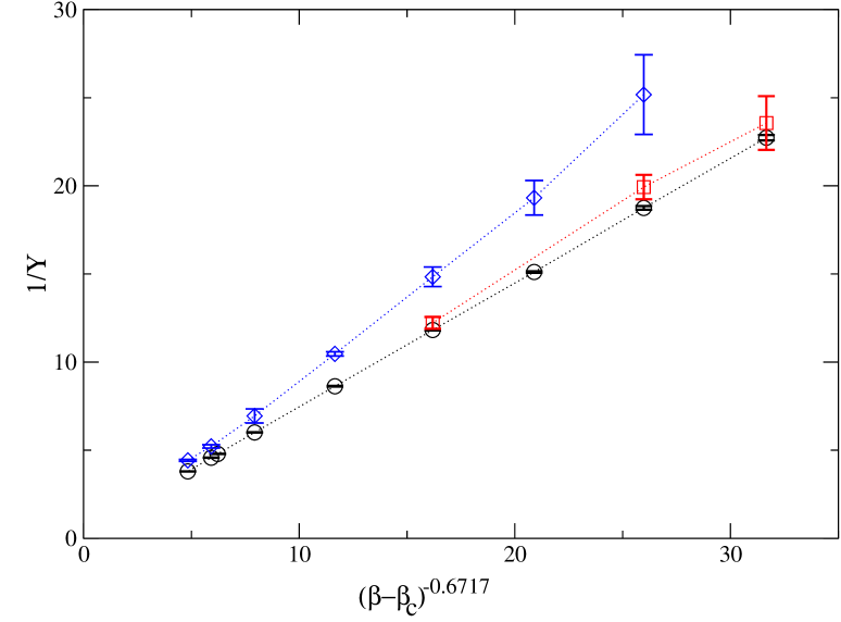
Figure 1: The inverse of the helicity modulus $\Upsilon$ is plotted as a function of $(\beta_{c}-\beta)^{-\nu}$ using the numerical value $\nu=0.6717$ for the exponent. Our results are given by the black circles; the data taken from ref. [9] are represented by red squares and the results of ref. [16] are given by blue diamonds. The dotted lines should only guide the eye.

6 Simulations in the high temperature phase

In the high temperature phase, we expect that the observables converge exponentially fast towards the thermodynamic limit. Therefore we have used lattice sizes that are large enough to ensure that the systematic error due to the finite lattice size is by far smaller than the statistical error of the observables that we have measured. We have checked that this is fulfilled for $L\gtrapprox 10\xi_{2nd}$. In fact for most of our the simulations we have chosen $L>12\xi_{2nd}$. Most of the simulations reported here were already performed in connection with refs. [10, 6]. The magnetic susceptibility $\chi$ and $F$ were measured using so called improved estimators; see e.g. ref. [22]. Note that these improved estimators are, in contrast to the naive ones, self-averaging. Hence, for large $L/\xi$ their statistical error is much smaller than that of the naive estimators. For the largest values of $\beta$ we have performed $2\times 10^{5}$ measurements. For each measurement we performed one Metropolis sweep and $n_{c}$ single cluster updates. The number $n_{c}$ of single cluster updates was chosen such that the average size of a cluster times $n_{c}$ is roughly equal to the number of sites of the lattice. The simulations for the largest lattice size $L=350$ took about one month on a 2 GHz Opteron CPU for each value of $\lambda$. Our results for the high temperature phase of the $\phi^{4}$ model at $\lambda=2.1$ and $\lambda=2.2$ and the XY model are summarized in tables 5, 6 and 7, respectively.

Table 5: Results for the high temperature phase of the 2-component $\phi^{4}$ model at $\lambda=2.1$. $\beta$ is the inverse temperature, $\xi_{2nd}$ the second moment correlation length, $\chi$ the magnetic susceptibility, $E$ the energy and $C$ the specific heat. For the definition of these quantities and detailed discussion see the text.

$\beta$	$\xi_{2nd}$	$2\chi$	$E$	$C$
0.40	1.07551(2)	0005.7056(2)	0.512689(10)	2.091(3)
0.41	1.15844(2)	0006.4486(2)	0.534164(10)	2.213(3)
0.42	1.25591(3)	0007.3867(3)	0.556926(12)	2.349(3)
0.43	1.37262(3)	0008.6013(4)	0.581128(13)	2.500(4)
0.44	1.51582(4)	0010.2280(5)	0.607060(12)	2.692(4)
0.45	1.69738(4)	0012.5045(5)	0.635073(7)	2.902(7)
0.455	1.80821(4)	0014.0117(5)	0.649978(6)	3.050(8)
0.46	1.93718(5)	0015.8770(8)	0.665592(8)	3.199(8)
0.465	2.08960(6)	0018.2377(8)	0.682020(8)	3.377(7)
0.47	2.27341(8)	0021.3070(13)	0.699359(9)	3.580(9)
0.475	2.50035(11)	0025.4333(18)	0.717754(9)	3.813(8)
0.48	2.79047(12)	0031.2425(22)	0.737430(9)	4.081(10)
0.485	3.17678(14)	0039.909(3)	0.758610(9)	4.385(11)
0.49	3.72370(19)	0053.998(5)	0.781682(7)	4.87(2)
0.493	4.1825(2)	0067.451(6)	0.796679(6)	5.09(3)
0.495	4.5763(2)	0080.177(6)	0.807259(6)	5.42(2)
0.50	6.1498(5)	141.899(17)	0.836367(6)	6.26(2)
0.503	8.0424(8)	238.88(5)	0.856373(7)	7.14(5)
0.505	10.4822(16)	400.38(11)	0.871351(8)	7.95(3)
0.506	12.6264(16)	575.74(14)	0.879580(6)	8.52(5)
0.507	16.318(4)	950.7(4)	0.888476(7)	9.43(8)
0.5075	19.498(6)	1347.1(8)	0.893283(9)	9.83(7)
0.508	24.845(8)	2164.6(1.4)	0.898418(6)	10.81(8)
0.5083	30.453(10)	3225.0(2.0)	0.901727(4)	11.32(9)

Table 6: Same quantities as in table 5 for $\lambda=2.2$.

$\beta$	$\xi_{2nd}$	$2\chi$	$E$	$C$
0.501	7.1723(5)	191.372(23)	0.849150(4)	6.681(10)
0.5035	9.5018(9)	330.80(6)	0.866864(5)	7.545(15)
0.5055	13.6104(21)	667.11(20)	0.882972(5)	8.62(4)
0.5067	19.710(5)	1376.2(6)	0.894014(6)	9.87(6)
0.50748	30.475(10)	3231.4(2.0)	0.902171(4)	11.41(9)

Table 7: Same quantities as in table 5 for the standard XY model.

$\beta$	$\xi_{2nd}$	$2\chi$	$E$	$C$
0.4	1.87550(7)	16.8465(10)	0.740797(15)	3.139(4)
0.41	2.18009(8)	22.0757(13)	0.773412(11)	3.388(5)
0.42	2.62528(12)	31.019(2)	0.809006(12)	3.736(6)
0.425	2.93916(12)	38.242(2)	0.828195(8)	3.957(6)
0.43	3.35803(15)	49.064(4)	0.848624(8)	4.231(7)
0.435	3.9514(2)	66.702(5)	0.870561(8)	4.561(6)
0.44	4.8769(2)	99.564(6)	0.894452(5)	5.014(8)
0.441	5.1305(2)	109.704(8)	0.899537(6)	5.139(7)
0.442	5.4184(2)	121.801(8)	0.904735(5)	5.242(8)
0.443	5.7489(3)	136.464(12)	0.910056(6)	5.390(7)
0.444	6.1327(3)	154.524(14)	0.915514(6)	5.542(7)
0.445	6.5851(4)	177.23(2)	0.921133(6)	5.704(8)
0.446	7.1286(5)	206.53(2)	0.926937(6)	5.874(10)
0.447	7.7960(4)	245.53(2)	0.932911(4)	6.104(9)
0.448	8.6402(4)	299.62(2)	0.939131(3)	6.342(9)
0.449	9.7488(6)	378.69(4)	0.945605(4)	6.644(10)
0.45	11.2871(7)	503.40(5)	0.952402(3)	6.959(10)

7 Universal amplitude ratios

In this section, we first define the amplitude ratios that we consider. Then we compute their values from the Monte Carlo data discussed in the previous sections. Finally we compare our results with those obtained by using other theoretical methods and experimental results obtained for the $\lambda$-transition of ⁴He.

7.1 Definition of the amplitude ratios

Here we define the amplitude ratios that we have studied. For a more comprehensive list see e.g. page 18 of ref. [2] or table 2 of ref. [23]. The first amplitude combination relates the correlation length in the high temperature phase with the helicity modulus which is defined in the low temperature phase:

$$R_{\Upsilon}\equiv f_{2nd,+}\Upsilon_{0}\;\;,$$ (22)

where the amplitudes are defined by

$$\xi_{2nd}=\simeq f_{2nd,+}(-t)^{-\nu}\;\;,\;\;\;\;\Upsilon\simeq\Upsilon_{0}t^{\nu}\;\;,\;\;\;\;(t>0)$$ (23)

where $\nu$ is the critical exponent of the correlation length. In this section we use, for computational convenience,

$$t=\beta-\beta_{c}$$ (24)

as definition of the reduced temperature. It has been shown in ref. [21] that the helicity modulus behaves as an inverse correlation length. The exponential correlation length $\xi_{exp}$, which describes the asymptotic decay of the correlation function, differs only slightly from $\xi_{2nd}$ which has been used here. Following ref. [14]:

$$\lim_{t\rightarrow 0}\frac{\xi_{exp}}{\xi_{2nd}}=1.000204(3)\;\;,\;\;\;\;(t<0)\;\;.$$ (25)

Next we consider

$$R_{B}\equiv\frac{C_{+}}{f_{2nd,+}^{3}B^{2}}\;\;,$$ (26)

where the amplitudes of the magnetic susceptibility and the correlation length in the high temperature phase are defined by eqs. (1,23), respectively. The amplitude of the magnetisation in the low temperature phase is defined by

$$\Sigma/2\simeq\left(Bt^{\beta}\right)^{2}\;\;,\;\;\;\;(t>0)\;\;.$$ (27)

As the third combination of amplitudes we consider

$$R_{\xi}^{+}\equiv(\alpha A^{+})^{1/3}f_{2nd,+}\;,$$ (28)

where the amplitude of the specific heat $C_{h}$ is given by

$$C_{h}\simeq A_{\pm}|t|^{-\alpha}+b\;.$$ (29)

The analytic background $b$ has to be taken into account, since the exponent of the specific heat $\alpha$ is negative for the three-dimensional XY universality class. The fourth combination of amplitudes that we consider is

$$R_{\xi}^{-}\equiv\frac{(\alpha A^{-})^{1/3}}{\Upsilon_{0}}\;\;.$$ (30)

In the case of $R_{\xi}^{+}$ and $R_{\xi}^{-}$ one has to be careful about the precise definition of the specific heat and the reduced temperature. We have checked that, due to a cancellation, our definitions of $R_{\xi}^{+}$ and $R_{\xi}^{-}$ indeed coincide with those used in the literature.

7.2 Numerical results

A straight forward way to obtain numerical estimates of amplitude ratios is to fit the numerical data for the various observables using ansätze like eqs. (1,23,27,29). Then the amplitude ratios are simply computed from the amplitudes that are obtained from these fits. Here instead we follow a strategy that had already been employed in ref. [24] where universal amplitude ratios for the three-dimensional Ising universality class had been computed. In order to eliminate the dependence of the result on the critical exponents, we consider ratios at a finite reduced temperature (24). As a first example let us consider

$$R_{\Upsilon}=\lim_{t\rightarrow 0}\xi_{2nd}(-t)\Upsilon(t)\;\;,\;\;\;\;(t>0)\;\;.$$ (31)

We have computed this product for the reduced temperatures $t=\beta_{low}-\beta_{c}$, where $\beta_{low}$ are those values of $\beta>\beta_{c}$ for which simulations have been performed. The values for $\Upsilon$ are taken from tables 2, 3 and 4. The tables 5, 6 and 7 contain no exact matches for $-t=\beta_{c}-\beta_{low}$. Therefore we computed $\xi_{2nd}$ at $-t$, i.e. at $\beta_{high}=2\beta_{c}-\beta_{low}$, by interpolating the results given in tables 5, 6 and 7. For this purpose, we took two values $\beta_{high,1}$ and $\beta_{high,2}$, where we have simulated, such that $\beta_{high,1}\leq\beta_{high}\leq\beta_{high,2}$ and $\beta_{high,2}-\beta_{high,1}$ is minimal. Then we interpolate linearly in $f_{2nd}(\beta)=\xi_{2nd}(\beta)(\beta_{c}-\beta)^{0.6717}$ to get $\xi_{2nd}$ at $\beta_{high}$. Our results for $\xi_{2nd}(-t)\Upsilon(t)$ are shown in figure 2. The statistical error of the product is completely dominated by the error of $\Upsilon$. Unfortunately, the error rapidly increases as we approach the critical temperature. We have checked that the error of $\xi_{2nd}(-t)\Upsilon(t)$ induced by the uncertainty of $\beta_{c}$ is negligible.

Based on RG theory (see e.g. ref. [23]), we expect that the product behaves as

$$\xi_{2nd}(-t)\Upsilon(t)=R_{\Upsilon}\;+\;b_{1}t^{\theta}+c_{1}t+d_{1}t^{\theta^{\prime}}+b_{2}t^{2\theta}+...\;\;.$$ (32)

The leading non-analytic correction is characterized by the exponent $\theta=\nu\omega$. As numerical values we take $\nu=0.6717(1)$ and $\omega=0.785(20)$ given in ref. [10]. This value of $\omega$ is consistent with e.g. the result of ref. [25] $\omega=0.789(11)$ from the perturbative expansion in $d=3$ and $\omega=0.802(18)$ from the $\epsilon$-expansion. There is little information on $\theta^{\prime}$ in the literature. We assume the value $\theta^{\prime}\approx 2\theta$ as obtained in ref. [26]. Since $2\theta\approx 1$, it is difficult to disentangle the three terms $c_{1}t$, $d_{1}t^{\theta^{\prime}}$ and $b_{2}t^{2\theta}$. Therefore we have used the ansatz

$$\xi_{2nd}(-t)\Upsilon(t)=R_{\Upsilon}\;+\;bt^{\theta}+ct$$ (33)

for our fits. Since $\lambda=2.1$ and $2.2$ are close to $\lambda^{*}$ we expect that $b$ is small for these values of $\lambda$.

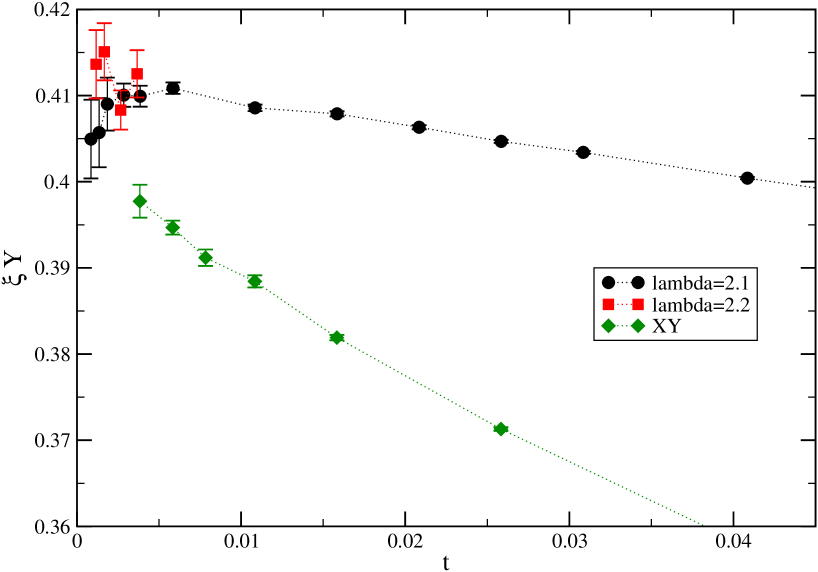
Figure 2: The product $\xi_{2nd}(-t)\Upsilon(t)$ for the $\phi^{4}$ model at $\lambda=2.1$, $\lambda=2.2$ and the XY model is plotted as a function of $t=\beta-\beta_{c}$, where we have taken $\beta_{c}=0.5091503$, $0.5083355$ and $0.4541655$ for the $\phi^{4}$ model at $\lambda=2.1$, $\lambda=2.2$ and the XY model, respectively. The dotted lines should only guide the eye.

We have fitted our results for the $\phi^{4}$ model at $\lambda=2.1$ and the XY model with the ansatz (33). In both cases, all available data points were included into the fit. In the case of $\lambda=2.2$ we have just averaged the available results, since we have only results for small values of $t$. The results of these fits are given in table 8. In all cases we get an $\chi/$d.o.f. close to 1. For $\lambda=2.1$, the coefficient $b$ of corrections $\propto t^{\theta}$ is within error-bars consistent with zero, confirming that $\lambda=2.1$ is close to $\lambda^{*}$. Within two standard deviations the result for $R_{\Upsilon}$ is consistent among the three different models. As our final result we quote

$$R_{\Upsilon}=0.411(2)\;\;,$$ (34)

where the error-bar is chosen such that the result for each of the models is covered.

Table 8: Fits of the product $\xi_{2nd}(-t)\Upsilon(t)$ using the ansatz (33) in the case of the $\phi^{4}$ model at $\lambda=2.1$ and the XY model. In the case of the $\phi^{4}$ model at $\lambda=2.2$ we have just averaged over all data that are available.

model	$R_{\Upsilon}$	$b$	$c$	$\chi/$d.o.f.
$\lambda=2.1$	0.4118(8)	–0.001(10)	–0.28(2)	1.12
$\lambda=2.2$	0.4092(11)	-	-	0.67
XY	0.4097(18)	–0.186(28)	–0.43(8)	0.22

Next we have computed the amplitude ratio $R_{B}$. Also here we have computed the ratio of observables at finite reduced temperatures:

$$R_{B}=\lim_{t\rightarrow 0}\frac{2\chi(-t)}{\xi_{2nd}(-t)^{3}\Sigma(t)}\;\;,\;\;\;\;(t>0)\;\;.$$ (35)

To this end we have followed a similar approach as for $R_{\Upsilon}$. We took the values $\Sigma(\beta_{low})$ given in tables 2, 3 and 4 for the $\phi^{4}$ model at $\lambda=2.1$ and $\lambda=2.2$ and the XY model, respectively. Then we computed $\xi_{2nd}(\beta_{high})$ and $\chi(\beta_{high})$ at $\beta_{high}=2\beta_{c}-\beta_{low}$ by interpolation of the results given in tables 5, 6 and 7, for the $\phi^{4}$ model at $\lambda=2.1$ and $\lambda=2.2$ and the XY model, respectively. The interpolation is done in an analogous way as discussed above. Our results are plotted in figure 3.

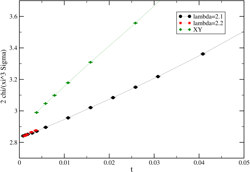
Figure 3: We plot the product $\frac{2\chi(-t)}{\xi_{2nd}(-t)^{3}\Sigma(t)}$ for the $\phi^{4}$ model at $\lambda=2.1$, $\lambda=2.2$ and the XY model as a function of $t=\beta-\beta_{c}$, where we have taken $\beta_{c}=0.5091503$, $0.5083355$ and $0.4541655$ for the $\phi^{4}$ model at $\lambda=2.1$, $\lambda=2.2$ and the XY model, respectively. The dotted lines should only guide the eye.

In principle, a similar ansatz as for $R_{\Upsilon}$ could be used here. However it turns out that the analytic background of the magnetic susceptibility has to be taken into account to get acceptable fits for a large range of $\beta$-values. Hence we have used the ansatz

$$\frac{2\chi(-t)}{\xi_{2nd}(-t)^{3}\Sigma(t)}=R_{B}+bt^{\theta}+ct+dt^{\gamma}\;\;.$$ (36)

The results of these fits are summarized in table 9.

Table 9: Fits of the $\phi^{4}$ model at $\lambda=2.1$ and the XY model using the ansatz (36). In the case of the XY model all available data are used, while in the case of the $\phi^{4}$ model all data up to $\beta=0.55$ are used; i.e. $\beta=0.58$ is skipped. In these fits $\beta_{c}=0.5091503$ and $\beta_{c}=0.4541655$ is used as input for the $\phi^{4}$ model at $\lambda=2.1$ and the XY model, respectively.

model	$R_{B}$	$b$	$c$	$d$	$\chi^{2}/$d.o.f.
$\lambda=2.1$	2.828(5)0	0.14(20)	7.2(2.1)	14.3(5)	1.44
XY	2.801(15)	3.2(5)	–3.1(4.7)	46.4(7.6)	2.21

To check the uncertainty due to the error of $\beta_{c}$, we have repeated the fits for shifted values of $\beta_{c}$ (both for computing the combination $\frac{2\chi(-t)}{\xi_{2nd}(-t)^{3}\Sigma(t)}$ as well as in the ansatz). We get $R_{B}=2.815(3)$, $2.797(16)$ using $\beta_{c}=0.5091509$ and $\beta_{c}=0.4541665$ for the $\phi^{4}$ model and the XY model, respectively.

We also performed fits for $\lambda=2.1$ and $2.2$ taking only analytic corrections into account:

$$\frac{2\chi(-t)}{\xi_{2nd}(-t)^{3}\Sigma(t)}=R_{B}+ct\;\;.$$ (37)

The results of these fits are given in table 10.

Table 10: Fits of the $\phi^{4}$ model at $\lambda=2.1$ and $\lambda=2.2$ using the ansatz (37). In the case of $\lambda=2.1$ we have taken into account all data up to $\beta=0.513$, while for $\lambda=2.2$ all available data have been used.

model	$R_{B}$	$c$	$\chi^{2}/$d.o.f.
$\lambda=2.1$	2.8329(26)	9.7(9)	0.24
$\lambda=2.2$	2.8276(29)	13.4(1.0)	1.13

Also here we have repeated the fits with shifted values of $\beta_{c}$. We get $R_{B}=2.83040(26)$ and $2.82494(29)$ using $\beta_{c}=0.5091509$ and $\beta_{c}=0.5083362$ for $\lambda=2.1$ and $\lambda=2.2$, respectively. Based on the fits with the ansatz (37) we arrive at our final result:

$$R_{B}=2.83(1)\;\;.$$ (38)

The error which is quoted covers the statistical error, the error due to the uncertainty of $\beta_{c}$ and the error due to residual leading corrections. The latter is estimated by the difference of the results for $\lambda=2.1$ and $\lambda=2.2$.

Finally we have computed $R_{\xi}^{+}$ and $R_{\xi}^{-}$. To this end we have analysed our very accurate data for the energy density. In the neighbourhood of the critical temperature, the energy density behaves as

$$E(t)=e_{ns}+c_{ns}t+a_{\pm}t^{1-\alpha}+...$$ (39)

with $a_{\pm}(1-\alpha)=A_{\pm}$. $e_{ns}$ and $c_{ns}$ are the non-singular contributions to the energy density and the specific heat at the transition temperature. Their numerical values had been accurately determined for the $\phi^{4}$ model at $\lambda=2.1$ and $2.2$ in ref. [6] using finite size scaling at the transition temperature. These results are given by [6]:

$$e_{ns}=0.913213(5)+20\times(\beta_{c}-0.5091503)+5\times 10^{-7}\times(1/\alpha+1/0.0151)$$ (40)

for $\lambda=2.1$ and

$$e_{ns}=0.913585(5)+20\times(\beta_{c}-0.5083355)+6\times 10^{-7}\times(1/\alpha+1/0.0151)$$ (41)

for $\lambda=2.2$. The results for the non-singular part of the specific heat are [6]:

$$c_{ns}=157.9(5)+147000\times(\beta_{c}-0.5091503)-2.1\times(1/\alpha+1/0.0151)$$ (42)

for $\lambda=2.1$ and

$$c_{ns}=155.6(4)+121000\times(\beta_{c}-0.5083355)-2.1\times(1/\alpha+1/0.0151)$$ (43)

for $\lambda=2.2$. Corresponding results for the XY model are not available.

Using these results we have computed the singular part of the energy density as

$$e_{s}(\beta)=E(\beta)-e_{ns}-c_{ns}(\beta-\beta_{c})\;,$$ (44)

where the numerical values for $E(\beta)$ are taken from tables 5 and 6 for the high temperature phase and from tables 2 and 3 for the low temperature phase. First we have computed

$$R_{\xi}^{+}=\lim_{t\rightarrow 0}\xi_{2nd}(t)\left[-\alpha(1-\alpha)e_{s}(t)(-t)\right]^{1/3}\;\;,\;\;\;\;(t<0)\;\;,$$ (45)

for the high temperature phase. Note that the combined critical exponent of the right hand side vanishes due to the hyperscaling relation $d\nu=2-\alpha$. Our results for this combination are given in figure 4.

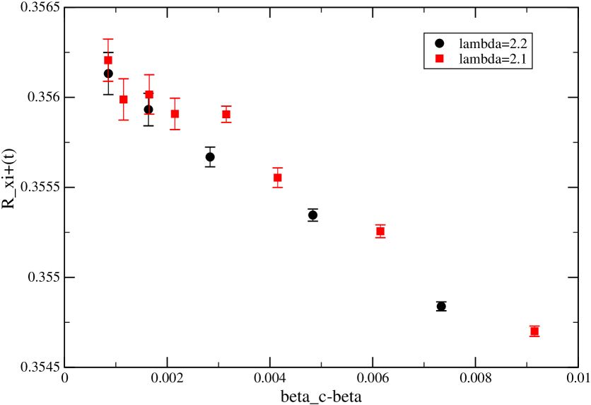
Figure 4: In this figure we show $R_{\xi}^{+}(t)=\xi_{2nd}(t)\left[-\alpha(1-\alpha)e_{s}(t)(-t)\right]^{1/3}$ for the $\phi^{4}$ model at $\lambda=2.1$ at $\lambda=2.2$. This product is plotted as a function of $-t=\beta_{c}-\beta$, where we have taken $\beta_{c}=0.5091503$ and $0.5083355$ for the $\phi^{4}$ model at $\lambda=2.1$ and $\lambda=2.2$, respectively. $e_{ns}$ and $c_{ns}$ are set to their central values. $\nu=0.6717$ is assumed.

In improved models, the corrections that are clearly visible, are to leading order due to terms $\propto t^{2}$ and $\propto t^{2-\alpha}$ missing in eq. (39). Our data do not allow to disentangle these two terms. Therefore we just linearly extrapolated our results for $\xi_{2nd}(t)\left[-\alpha(1-\alpha)e_{s}(t)(-t)\right]^{1/3}$ to $t=0$. We get from the extrapolation of the 5 largest values of $\beta$ the results $R_{\xi}^{+}=0.35616(11)$ and $R_{\xi}^{+}=0.35626(6)$ for $\lambda=2.1$ and $\lambda=2.2$, respectively. The error of $R_{\xi}^{+}$ is actually dominated by the error induced by the uncertainty of our input parameters, $e_{ns}$, $c_{ns}$, $\beta_{c}$ and $\alpha$. In order to estimate this error, we have repeated the whole procedure for shifted values of these input parameters. In particular, we have replaced $e_{ns}$ by $e_{ns}+\mbox{error}$ and similarly for the other input parameters. The errors obtained this way are very similar for the two values of $\lambda$. The largest contribution to the error originates from the uncertainty in $c_{ns}$ followed by $\beta_{c}$, $\alpha$ and $e_{ns}$. Note that the relatively small error due to the uncertainty of $\alpha$ is due to a cancellation of the variation of the $\alpha$ that appears explicitly in the definition of $R_{\xi}^{+}$ and that due to the dependence of $c_{ns}$ (42,43) on $\alpha$. Adding up all these errors we arrive at our final estimate

$$R_{\xi}^{+}=0.3562(10)\;\;.$$ (46)

Finally we computed

$$R_{\xi}^{-}=\lim_{t\rightarrow 0}\frac{1}{\Upsilon(t)}\left[-\alpha(1-\alpha)e_{s}(t)\;(-t)\right]^{1/3}\;\;,\;\;\;\;(t>0)\;\;.$$ (47)

Note that in the low temperature phase $e_{s}(t)$ is negative, hence the product contained in $[]$ is positive. Our numerical results for the $\phi^{4}$ model at $\lambda=2.1$ and $2.2$ are shown in figure 5. Unfortunately the statistical error blows up for small reduced temperatures. This is mainly due to the fact that the relative error of the helicity modulus $\Upsilon$ rapidly increases as the critical temperature is approached. In the case of $\lambda=2.1$, the value of $R_{\xi}^{-}$ stays essentially constant over the range $0.01<\beta-\beta_{c}<0.03$. Therefore we regard the apparent increase of the value at small $\beta-\beta_{c}$ as a statistical accident. This is confirmed by the fact that for $\lambda=2.2$ no such trend can be seen. Motivated by this consideration, we take our final result for $R_{\xi}^{-}$ as the average over all data with $\beta-\beta_{c}<0.005$. We get $R_{\xi}^{-}=0.852(2)$ and $0.848(3)$ for $\lambda=2.1$ and $\lambda=2.2$, respectively. As our final result we take the average over the two values of $\lambda$:

$$R_{\xi}^{-}=0.850(5)\;\;.$$ (48)

The error-bar is chosen such that the results of both values of $\lambda$, including their individual error-bars, are covered. We have also checked the possible error due to the uncertainty of the input parameters $\alpha$, $\beta_{c}$, $e_{ns}$ and $c_{ns}$. Here, in contrast to $R_{\xi}^{+}$, these errors can be ignored. Actually the result for $R_{\xi}^{-}$ is virtually independent on $\alpha$. Using the experimental value $\alpha=-0.0127$ [3, 4] instead of our theoretical one, the result for $R_{\xi}^{+}$ changes only in the fourth digit. This is due to the fact that the variation of $\alpha$ that appears explicitly in the definition of $R_{\xi}^{+}$ essentially cancels with that of $c_{ns}$ (42,43).

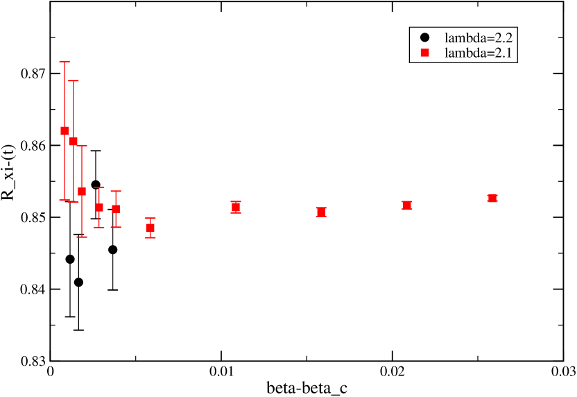
Figure 5: In this figure we give $R_{\xi}^{-}(t)=\Upsilon(t)^{-1}\left[-\alpha(1-\alpha)e_{s}(t)\;(-t)\right]^{1/3}$ for the $\phi^{4}$ model at $\lambda=2.1$ at $\lambda=2.2$. It is plotted as a function of $t=\beta-\beta_{c}$, where we have taken $\beta_{c}=0.5091503$ and $0.5083355$ for the $\phi^{4}$ model at $\lambda=2.1$ and $\lambda=2.2$, respectively. $e_{ns}$ and $c_{ns}$ are set to their central values. $\nu=0.6717$ is assumed.

7.3 Comparison with other theoretical and experimental results

In table 11 we have summarized results from the literature that where obtained by different theoretical methods and from experiments on the $\lambda$-transition of ⁴ He. Essentially we followed table 22 of ref. [23].

For $R_{\xi}^{+}$ most theoretical results are in reasonable agreement among each other. In the case of the field theoretic expansion in three dimensions [27, 28] there is a discrepancy with our result that is somewhat larger than the combined error. There is no experimental result for this amplitude ratio, since there is no direct experimental access to the correlation length of ⁴He in the high temperature phase. The authors of ref. [16] quote their Monte Carlo result as a function of $\alpha$: $R_{\xi}^{+}=0.3382(14)-0.717(96)\alpha+0.87(1.13)\alpha^{2}$. We have inserted $\alpha=-0.0151$ to get the value quoted in table 11. It differs by about 3 times the combined error from our result.

In the case of $R_{\xi}^{-}$ our result is in perfect agreement with the experimental number given in table IV of ref. [34]. It is interesting to note that also the experimental value of $R_{\xi}^{-}$ shows very little dependence on the value of $\alpha$ that is assumed in the analysis; the authors of ref. [34] arrive at $R_{\xi}^{-}=0.86$ and $R_{\xi}^{-}=0.84$ using $\alpha=-0.007$ and $\alpha=-0.025$, respectively, instead of their preferred value $\alpha=-0.016$. They do not explicitly quote an error for their estimate of $R_{\xi}^{-}$. In section III.B. they write however that $(R_{\xi}^{-})^{3}$ is constant within $5\%$ over the entire range of pressures from 0 to 30 bars. In the review [2] the result of ref. [34] is quoted as $R_{\xi}^{-}=0.85\pm 0.02$. Concerning theory, there is a discrepancy by about twice the combined error with the field theoretic result [31, 32]. The error of the result obtained by the $\epsilon$-expansion [29, 33, 2] is quite large. The authors of ref. [16] quote their Monte Carlo result as $R_{\xi}^{-}=1.1580-0.696\alpha+0.97\alpha^{2}\pm 0.036$. The huge difference compared with our result is likely due to the difference in the estimates of $\Upsilon$ as discussed in section 5.

Table 11: We summarize results obtained by using different theoretical methods and experiments on the $\lambda$-transition of ⁴He. MC denotes Monte Carlo simulations of lattice models, HT the high temperature series expansion of lattice models, IHT-PR the high temperature series expansion of improved lattice models combined with the parametric representation of the equation of state, d=3 exp the field theoretic expansion in three dimensions fixed and $\epsilon$ exp the $\epsilon$-expansion. For convenience, we have added our present results in the second column of the table. A detailed discussion is given in the text.

	MC	HT,IHT-PR	d=3 exp	$\epsilon$ exp	Experiment
$R_{\xi}^{+}$	0.3562(10)	0.355(3) [14]	0.3606(20) [28, 27]	0.36 [29]
	0.349(5) [16]	0.361(4) [30]
$R_{\xi}^{-}$	0.850(5)		0.815(10) [31, 32]	1.0(2) [29, 33, 2]	0.85(2) [34]
	1.180(36) [16]
$R_{c}^{+}$	0.128(2)	0.127(6) [14]	0.123(3) [35]	0.106 [36, 37, 38]
	0.128(4) [16]
$R_{\Upsilon}$	0.411(2)			0.27 [33]	0.39 [40, 41, 33]
	0.293(9) [16]			0.33 [29, 39]	0.41 [40, 41, 29]

In the literature our universal amplitude ratio $R_{B}$ is not discussed. Instead one finds

$$R_{c}^{+}=\frac{\alpha A_{+}C_{+}}{B^{2}}\;\;.\;$$ (49)

It can be expressed as

$$R_{c}^{+}=(R_{\xi}^{+})^{3}R_{B}=0.128(2)\;\;.$$ (50)

where the error is dominated by the error of $R_{\xi}^{+}$. Our present result is in good agreement with that obtained in ref. [14] using the high temperature expansion of improved models in combination with the parametric representation of the equation of state. It also agrees with ref. [16], where a combination of Monte Carlo simulations and the parametric representation of the equation of state was used. In ref. [16] $R_{c}^{+}$ is given as a function of $\alpha$. The value in our table is at $\alpha=-0.0151$. Again there is a discrepancy with the field theoretic result [35] that is slightly larger than the combined error. The $\epsilon$-expansion for $R_{c}^{+}$ has been computed up to O($\epsilon^{2}$) [36, 37, 38]. The number given in the table is obtained by simply setting $\epsilon=1$. There is no experimental result for $R_{c}^{+}$, since there is no experimental access in ⁴He to the analogue of the magnetisation in spin models.

In the case of $R_{\Upsilon}$ we see the largest differences among the results obtained by using theoretical methods. The Monte Carlo result, quoted in eq. (97) of ref. [16], differs by more then 10 times the combined error from ours. This huge difference can be traced back to the discrepancy in $\Upsilon$ at given values of $\beta$ as discussed in section 5. Hohenberg et al. [33] have computed $R_{\Upsilon}$ by using the $\epsilon$-expansion to O($\epsilon$). Bervillier [29] extended the calculation up to O($\epsilon^{2}$). Okabe and Ideura [39] corrected the calculation of Bervillier, which does however not change the numerical value, and computed the $1/N$-expansion resulting in $R_{\Upsilon}=0.14$ for $N=2$.

There are no direct experimental results for the correlation length in the high temperature phase of ⁴He. Instead one might use the data for the specific heat in combination with the theoretical result for $R_{\xi}^{+}$ to arrive at the amplitude of the correlation length. This way, using $R_{\xi}^{+}=0.36$ and the experimental results of refs. [40, 41], Hohenberg et al. [33] arrive at $R_{\Upsilon}=0.39$. Bervillier noted, see section III.A. of [29], that there is an error in the experimental value of the amplitude of the transversal correlation length used by Hohenberg et al. [33]. He arrives at the corrected value $R_{\Upsilon}=0.41$. It would certainly be worth while to redo this calculation using most recent experimental data; e.g. those of ref. [3, 4] for the specific heat and our estimate of $R_{\xi}^{+}$.

8 Summary and Conclusions

In this paper we have computed universal amplitude ratios for the three dimensional XY universality class. These results are based on Monte Carlo simulations of the three dimensional XY model and the $\phi^{4}$-model at $\lambda=2.1$ and $\lambda=2.2$. Note that these values of $\lambda$ are close to $\lambda^{*}=2.15(5)$ [10], where leading corrections to scaling vanish. We performed simulations in the low and the high temperature phase of these models. Extracting results for the thermodynamic limit, one has to take into account the effect of the Goldstone mode in the low temperature phase. For a discussion see section 4.

Our results for universal amplitude ratios for the three-dimensional XY universality class are throughout more precise than previous theoretical results. They are obtained in a rather direct way, making hidden systematic errors unlikely. When available, our results agree nicely with experimental ones obtained for the $\lambda$-transition of ⁴He, giving further confirmation to the fact that this transition shares the three-dimensional XY universality class.

The numerical results obtained here for the correlation length $\xi_{2nd}$, the helicity modulus $\Upsilon$, the energy density $E$ and the specific heat set the stage also for the study of the specific heat or the Casimir force in confined geometries using improved models.

9 Acknowledgements

I like to thank Andrea Pelissetto and Ettore Vicari for remarks on the literature. The simulations were mainly carried out at the computer centre of the Dipartimento di Fisica dell’Università di Pisa. This work was partially supported by the DFG under grant No JA 483/23-1.

References

- [1] Wilson K G and Kogut J, The renormalization group and the -expansion, 1974 Phys. Rep. C 12 75
- [2] Privman V, Hohenberg P C, Aharony A, Universal Critical-Point Amplitude Ratios, in Phase Transitions and Critical Phenomena, edited by C. Domb and J.L. Lebowitz (Academic Press, New York, 1991) Vol. 14.
- [3] Lipa J A, Swanson D R, Nissen J A, Chui T C P and Israelsson U E, Heat Capacity and Thermal Relaxation of Bulk Helium very near the -Point, 1996 Phys. Rev. Lett. 76 944
- [4] Lipa J A, Nissen J A, Stricker D A, Swanson D R and Chui T C P, Specific heat of liquid helium in zero gravity very near the -point, 2003 Phys. Rev. B 68 74518 [cond-mat/0310163]
- [5] Barmatz M, Hahn I, Lipa J A, and Duncan R V, Critical phenomena in microgravity: Past, present, and future, 2007 Rev. Mod. Phys. 79 1
- [6] Hasenbusch M, The three-dimensional XY universality class: A high precision Monte Carlo estimate of the universal amplitude ratio , 2006 J. Stat. Mech. P08019 [cond-mat/0607189]
- [7] Hasenfratz P and Leutwyler H, Goldstone Boson Related Finite Size Effects In Field Theory And Critical Phenomena With O(N) Symmetry, 1990 Nucl. Phys. B 343 241
- [8] Dimitrović I, Hasenfratz P, Nager J and Niedermayer F, Finite size effects, Goldstone bosons and critical exponents in the Heisenberg model, 1991 Nucl. Phys. B 350 893
- [9] Tominaga S and Yoneyama H, Chiral perturbation theory, finite-size effects, and the three-dimensional XY model, 1995 Phys. Rev. B 51 8243 [hep-lat/9408001]
- [10] Campostrini M, Hasenbusch M, Pelissetto A, and Vicari E, Theoretical estimates of the critical exponents of the superfluid transition in He4 by lattice methods, 2006 Phys. Rev. B 74 144506 [cond-mat/0605083]
- [11] Bittner E and Janke W, Nature of Phase Transitions in a Generalized Complex Model, 2005 Phys. Rev. B 71 024512 [cond-mat/0501468]
- [12] Chen J H, Fisher M E, and Nickel B G, Unbiased Estimation of Corrections to Scaling by Partial Differential Approximants, 1982 Phys. Rev. Lett. 48 630
- [13] Hasenbusch M and Török T, High precision Monte Carlo study of the 3D XY-universality class, 1999 J. Phys. A 32 6361 [cond-mat/9904408]
- [14] Campostrini M, Hasenbusch M, Pelissetto A, Rossi P, and Vicari E, Critical behavior of the three-dimensional XY universality class, 2001 Phys. Rev. B 63 214503 [cond-mat/0010360]
- [15] Ballesteros H G, Fernandez L A, Martin-Mayor V, and Munoz-Sudupe A, Finite size effects on measures of critical exponents in O(N) models, 1996 Phys. Lett. B 387 125 [cond-mat/9606203]
- [16] Cucchieri A, Engels J, Holtmann S, Mendes T and Schulze T, Universal amplitude ratios from numerical studies of the three-dimensional O(2) model, 2002 J. Phys. A 35 6517 [cond-mat/0202017]
- [17] Deng Y, Blöte H W J, and Nightingale M P, Surface and bulk transitions in three-dimensional O(n) models, 2005 Phys. Rev. E 72 016128 [cond-mat/0504173]
- [18] Wolff U, Collective Monte Carlo Updating for Spin Systems 1989 Phys. Rev. Lett. 62 361
- [19] Brower R C and Tamayo P, Embedded dynamics for theory, 1989 Phys. Rev. Lett. 62 1087
- [20] Li Y-H and Teitel S, Finite-size scaling study of the three-dimensional classical XY model, 1989 Phys. Rev. B 40 9122
- [21] Fisher M E, Barber M N, and Jasnow D, Helicity Modulus, Superfluidity, and Scaling in Isotropic Systems, 1973 Phys. Rev. A 8 1111
- [22] Wolff U, Continuum Behavior In The Lattice O(3) Nonlinear Sigma Model, 1989 Phys. Lett. B 222 473
- [23] Pelissetto A and Vicari E, Critical Phenomena and Renormalization-Group Theory, 2002 Phys. Rept. 368 549 [arXiv:cond-mat/0012164]
- [24] Caselle M and Hasenbusch M, Universal amplitude ratios in the three-dimensional Ising model 1997 J. Phys. A 30 4963 [hep-lat/9701007]
- [25] Guida R and Zinn-Justin J, Critical exponents of the N-vector model, 1998 J. Phys. A 31, 8103 [cond-mat/9803240]
- [26] Newman K E and Riedel E K, Critical exponents by the scaling-field method: The isotropic N-vector model in three dimensions, 1984 Phys. Rev. B 30 6615
- [27] Bervillier C and Godrèche C, Universal combination of critical amplitudes from field theory 1980 Phys. Rev. B 21 5427
- [28] Bagnuls C and Bervillier C, Nonasymptotic critical behavior from field theory at d=3: The disordered-phase case, 1985 Phys. Rev. B 32 7209
- [29] Bervillier C, Universal relations among critical amplitude. Calculations up to order for systems with continuous symmetry, 1976 Phys. Rev. B 14 4964
- [30] Butera P and Comi M, Critical specific heats of the N-vector spin models on the simple cubic and bcc lattices, 1999 Phys. Rev. B 60 6749 [hep-lat/9903010]
- [31] Burnett S S C, Strösser M and Dohm V, Minimal renormalization without -expansion: Amplitude functions for O(n) symmetric systems in three dimensions below ,1997 Nucl. Phys. B 504 665 [cond-mat/9703062]; addendum 1998 Nucl. Phys. B 509 729
- [32] Strösser M, Mönnigmann M, and Dohm V, Universal amplitude ratios for the superfluid transition of 4He, 2000 Physica B 284-288 41
- [33] P. C. Hohenberg, A. Aharony, B. I. Halperin and E. D. Siggia, Two-scale-factor universality and the renormalization group, 1976 Phys. Rev. B 13 2986
- [34] Singasaas A and Ahlers G, Universality of static properties near the superfluid transition in 4He, 1984 Phys. Rev. B 30 5103
- [35] Strösser M, Larin S A, and Dohm V, Minimal renormalization without -expansion: Three-loop amplitude functions of the O(n) symmetric -theory in three dimensions below , 1999 Nucl. Phys. B 540 654 [cond-mat/9806103]
- [36] R. Abe and S. Hikami, Consistency for a Critical Amplitude Ratio in and Expansions, 1977 Prog. Theor. Phys. 57 1538
- [37] Abe R and Masutani M, Note on -Expansion for Critical Amplitude Ratio , 1978 Prog. Theor. Phys. 59 672
- [38] Aharony A and Hohenberg P C, Universal relations among thermodynamic critical amplitudes, 1976 Phys. Rev. B 13 3081
- [39] Okabe Y and Ideura K, Critical Amplitude Ratio in and -Expansions, 1981 Prog. Theor. Phys. 66 1959
- [40] Greywall D S and Ahlers G, Second-Sound Velocity and Superfluid Density in 4He under Pressure near , 1973 Phys. Rev. A 7 2145
- [41] Ahlers G, Thermodynamics and Experimental Tests of Static Scaling and Universality near the Superfluid Transition in He4 under Pressure, 1973 Phys. Rev. A 8 530; Mueller K H, Pobell F and Ahlers G, Thermal-Expansion Coefficient and Universality near the Superfluid Transition of 4He under Pressure, 1975 Phys. Rev. Lett. 34 513