Evolving Lorentzian wormholes supported by phantom matter with constant state parameters

Abstract

Abstract: In this paper we study the possibility of sustaining an evolving wormhole via exotic matter made out of phantom energy. We show that this exotic source can support the existence of evolving wormhole spacetimes. Explicitly, a family of evolving Lorentzian wormholes conformally related to another family of zero-tidal force static wormhole geometries is found in Einstein gravity. Contrary to the standard wormhole approach, where first a convenient geometry is fixed and then the matter distribution is derived, we follow the conventional approach for finding solutions in theoretical cosmology. We derive an analytical evolving wormhole geometry by supposing that the radial tension (which is negative to the radial pressure) and the pressure measured in the tangential directions have barotropic equations of state with constant state parameters. At spatial infinity this evolving wormhole, supported by this anisotropic matter, is asymptotically flat, and its slices $t=$ constant are spaces of constant curvature. During its evolution the shape of the wormhole expands with constant velocity, i.e without acceleration or deceleration, since the scale factor has strictly a linear evolution.

I Introduction

Wormholes, as well as black holes, are an extraordinary consequence of Einstein’s equations of general relativity. During recent last decades, there has been a considerable interest in the field of wormhole physics. Two separate directions emerged: one relating to Euclidean signature metrics Coleman ; Strominger and the other concerned with Lorentzian ones. The interest has been focused on traversable Lorentzian wormholes (which have no horizons, allowing two-way passage through them), and were especially stimulated by the pioneering works of Morris, Thorne and Yurtsever Morris , where static, spherically symmetric Lorentzian wormholes were defined and considered to be an exciting possibility for constructing time machine models with these exotic objects, for backward time travel (see also Novikov ).

Most of the efforts are directed to study static configurations that must have a number of specific properties in order to be traversable. The most striking of these properties is the violation of energy conditions. This implies that the matter supporting the traversable wormholes is exotic Morris ; Visser , which means that it has very strong negative pressures, or even that the energy density is negative, as seen by static observers. However, one can also consider time-dependent wormhole configurations, such as rotating wormholes Teo or evolving wormholes in a cosmological background Kar1 ; Kar2 ; Lobo ; Arellano .

Lower Kim and higher dimensional wormholes have also been considered by several authors. Euclidean wormholes have been studied by Gonzales–Diaz and by Jianjun and Sicong Gonzales for example. The Lorentzian ones have been studied in the context of the n–dimensional Einstein theory Cataldo or Einstein–Gauss–Bonnet theory of gravitation Biplab . Evolving higher dimensional wormholes also have been studied Sayan .

The theoretical construction of wormhole geometries is usually performed by using the method where, in order to have a desired metric, one is free to fix the form of the metric functions, such as the redshift and shape functions, or even the scale factor for evolving wormholes. In this way one may have a redshift function without horizons, or with a desired asymptotic. Unfortunately, in this case we can obtain expressions for the energy and pressure densities which are physically unreasonable.

In this paper we shall follow the conventional method for finding solutions in general relativity, and used also in theoretical cosmology. We shall prescribe the matter content by specifying the equations of state of the radial and the tangential pressures and then we solve the Einstein field equations in order to find the redshift and shape functions together with the scale factor. Specifically we shall consider that these pressures obey barotropic equations of state with constant state parameters. In other words, we shall find all evolving wormhole geometries which have the radial and the tangential pressures proportional to the energy density.

The outline of the present paper is as follows: In Sec. II we briefly review some important aspects of static wormholes and give the definition of evolving wormholes. In Sec. III we find the metric of evolving wormholes with pressures obeying barotropic equations of state with constant state parameters. In Sec. IV the properties of the obtained wormhole geometry are studied. We use the metric signature ($-+++$) and set $c=1$.

II Evolving Lorentzian wormholes

II.1 Characterization of a static Lorentzian wormhole

Before treating evolving Lorentzian wormholes let us review the static ones. The metric ansatz of Morris and Thorne Morris for the spacetime which describes a static Lorentzian wormhole is given by

$$ds^{2}=-e^{2\Phi(r)}dt^{2}+\frac{dr^{2}}{1-\frac{b(r)}{r}}+r^{2}(d\theta^{2}+sin^{2}\theta d\varphi^{2}),$$ (1)

where $\Phi(r)$ is the redshift function, and $b(r)$ is the shape function since it controls the shape of the wormhole.

Morris and Thorne have discussed in detail the general constraints on the functions $b(r)$ and $\Phi(r)$ which make a wormhole Morris :

Constraint 1: A no–horizon condition, i.e. $e^{\Phi(r)}$ is finite throughout the space–time in order to ensure the absence of horizons and singularities.

Constraint 2: The shape function $b(r)$ must obey at the throat $r=r_{0}$ the following condition: $b(r_{0})=r_{0}$, being $r_{0}$ the minimum value of the $r$–coordinate. In other words $g^{-1}_{rr}(r_{0})=0$.

Constraint 3: Finiteness of the proper radial distance, i.e.

$$\frac{b(r)}{r}\leq 1,$$ (2)

(for $r\geq r_{0}$) throughout the space–time. This is required in order to ensure the finiteness of the proper radial distance $l(r)$ defined by

$$l(r)=\pm\int^{r}_{r_{0}}\frac{dr}{\sqrt{1-b(r)/r}}.$$ (3)

The $\pm$ signs refer to the two asymptotically flat regions which are connected by the wormhole. The equality sign in (2) holds only at the throat.

Constraint 4: Asymptotic flatness condition, i.e. as $l\rightarrow\pm\infty$ (or equivalently, $r\rightarrow\infty$) then $b(r)/r\rightarrow 0$.

Notice that these constraints provide a minimum set of conditions which lead, through an analysis of the embedding of the spacelike slice of (1) in a Euclidean space, to a geometry featuring two asymptotically flat regions connected by a bridge.

Although asymptotically flat wormhole geometries have been extensively considered in the literature, one can study however other asymptotic behaviors that are worth considering. For instance asymptotically anti–de Sitter wormholes may be also of particular interest Barcelo .

II.2 Evolving Lorentzian wormholes

We shall consider a simple generalization of the original Morris and Thorne metric (1) to a time-dependent metric given by

$$ds^{2}=$$

$$-e^{2\Phi(r)}dt^{2}+a(t)^{2}\left(\frac{dr^{2}}{1-\frac{b(r)}{r}}+r^{2}(d\theta^{2}+sin^{2}\theta d\varphi^{2})\right),$$ (4)

where $a(t)$ is the scale factor of the universe. Note that the essential characteristics of a wormhole geometry are still encoded in the spacelike section. It is clear that if $b(r)\rightarrow 0$ and $\Phi(r)\rightarrow 0$ the metric (II.2) becomes the flat Friedmann-Robertson-Walker (FRW) metric, and as $a(t)\rightarrow const$ it becomes the static wormhole metric (1).

In general, in order to construct an evolving wormhole, one has to specify or determine the red–shift function $\Phi(r)$, the shape function $b(r)$ and the scale factor $a(t)$. So, one of them may be chosen by fiat and the others may be determined by implementing some physical conditions. For example in Ref. Roman15 an exponential scale factor is considered in order to explore the possibility that inflation might provide a natural mechanism for the enlargement of an initially small (possibly submicroscopic) wormhole to macroscopic size. In Ref. Kar1 also different choices for the scale factor $a(t)$ are considered and the constraints are found on the minimum values of the throat radii.

In this paper we shall require that $\Phi(r)=0$ in order to have a family of evolving Lorentzian wormholes conformally related to another family of zero–tidal force static wormholes, and to ensure that there is no horizon. We also shall require that the radial tension, which is the negative of the radial pressure, and the pressure measured in the tangential directions (orthogonal to the radial direction) have barotropic equations of state with constant state parameters. These simple choices will permit us to find explicit analytical expressions, by solving the Einstein field equations, for the shift and shape functions, the scale factor, and the energy and pressure densities.

III Einstein field equations for the evolving Lorentzian wormholes

In order to simplify the analysis and the physical interpretation (with $\Phi(r)=0$) we now introduce the proper orthonormal basis as

$$ds^{2}=-\theta^{(t)}\theta^{(t)}+\theta^{(r)}\theta^{(r)}+\theta^{(\theta)}\theta^{(\theta)}+\theta^{(\varphi)}\theta^{(\varphi)},$$ (5)

where the basis one–forms $\theta^{(\alpha)}$ are given by

$$\theta^{(t)}=dt;\,\,\,\,\,\theta^{(r)}=\frac{a(t)\,dr}{\sqrt{1-\frac{b(r)}{r}}};$$

$$\theta^{(\theta)}=a(t)\,rd\theta;\,\,\,\,\,\theta^{(\varphi)}=a(t)\,r\,sin\,\theta\,d\varphi.$$ (6)

These basis one–forms are related to the following set of orthonormal basis vectors defined by

$$e_{\hat{t}}=e_{t};\,\,\,\,\,e_{\hat{r}}=a(t)^{-1}\sqrt{1-\frac{b(r)}{r}}\,e_{r};$$

$$e_{\hat{\theta}}=a(t)^{-1}r^{-1}\,e_{\theta};e_{\hat{\varphi}}=a(t)^{-1}\,r^{-1}\,sin^{-1}\theta\,e_{\varphi}.$$ (7)

This basis represents the proper reference frame of a set of observers who always remain at rest at constant $r$, $\theta$, $\varphi$ Roman15 .

For these basises the only nonzero components of the energy–momentum tensor $T_{(\mu)(\nu)}$ are precisely the diagonal terms $T_{(t)(t)}$, $T_{(r)(r)}$, $T_{(\theta)(\theta)}$ and $T_{(\varphi)(\varphi)}$, which are given by

$$T_{(t)(t)}=\rho(t,r),T_{(r)(r)}=p_{r}(t,r)=-\tau(t,r),$$

$$T_{(\theta)(\theta)}=T_{(\varphi)(\varphi)}=p_{{}_{l}}(t,r),$$ (8)

where the quantities $\rho(t,r)$, $p_{r}(t,r)$, $\tau(t,r)(=-p_{r}(t,r))$, and $p_{{}_{l}}(t,r)(=p_{\varphi}(t,r)=p_{\theta}(t,r))$ are respectively the energy density, the radial pressure, the radial tension per unit area, and lateral pressure as measured by observers who always remain at rest at constant $r$, $\theta$, $\varphi$.

Thus for the spherically symmetric wormhole metric (II.2), with $\Phi(r)=0$, the Einstein equations are given by

$$\kappa\rho(t,r)=3H^{2}+\frac{b^{\prime}}{a^{2}r^{2}},$$ (9)

$$\kappa p_{r}(t,r)=-\kappa\tau(t,r)=-2\,\frac{\ddot{a}}{a}-H^{2}-\frac{b}{a^{2}r^{3}},$$ (10)

$$\kappa p_{{}_{l}}(t,r)=-2\,\frac{\ddot{a}}{a}-H^{2}+\frac{b-rb^{\prime}}{2a^{2}r^{3}},$$ (11)

where $\kappa=8\pi G$, $H=\dot{a}/a$, and an overdot and a prime denote differentiation with respect to $t$ and $r$ respectively.

Now we shall require that the radial tension and the lateral pressure have barotropic equations of state. Thus we can write

$$\tau(t,r)=-p_{r}(t,r)=-\omega_{r}\,\rho(t,r),$$

$$p_{{}_{l}}(t,r)=\omega_{{}_{l}}\,\rho(t,r),$$ (12)

where $\omega_{r}$ and $\omega_{{}_{l}}$ are constant state parameters. Clearly, the requirement (III) with $\omega_{r}=\omega_{{}_{l}}$ allows us to connect the evolving wormhole spacetime (II.2) with the standard FRW cosmologies, where the isotropic pressure density is expressed as $p=\omega\rho$, with constant state parameter $\omega$ (=$\omega_{r}=\omega_{{}_{l}}$).

Now, using the conservation equation $T^{\mu}_{\,\,\,\,\nu;\mu}=0$, we have that

$$\dot{\rho}+H(3\rho+p_{r}+2p_{{}_{l}})=0,$$ (13)

$$\frac{2(p_{{}_{l}}-p_{r})}{r}=\frac{2(p_{{}_{l}}+\tau)}{r}=p^{\,\prime}_{r},$$ (14)

which may be interpreted as the conservation equation and the relativistic Euler equation (or the hydrostatic equation for equilibrium for the matter supporting the wormhole) respectively. From these equations we see that for $\omega_{r}=\omega_{{}_{l}}=\omega$, i.e. $p_{{}_{l}}=p_{r}=p$, we have the standard cosmological conservation equation $\dot{\rho}+3H(\rho+p)=0$, with $p^{\,\prime}_{r}=0$, so if we want to isotropize the pressure with a barotropic equation of state and constant state parameters, then we can not have a pressure of the form $p=p(t,r)$, it will depend only on time $t$.

Now, with the help of the conservation equation and the relativistic Euler equation we can easily solve the Einstein equations (9)–(11). From the structure of these conservation equations we see that one can write the energy density in the form $\rho(t,r)=\rho_{t}(t)\rho_{r}(r)$. Thus from the conservation equation we obtain

$$\rho_{t}(t)=C_{1}a^{-(3+\omega_{r}+2\omega_{{}_{l}})},$$ (15)

where $C_{1}$ is an integration constant. Now taking into account Eq. (III), from Eq. (14) we have that

$$\rho_{r}(r)=C_{2}r^{2(\omega_{{}_{l}}-\omega_{r})/\omega_{r}},$$ (16)

where $C_{2}$ is an integration constant. Thus from expressions (15) and (16) we can write for the energy density

$$\rho(t,r)=C\,r^{2(\omega_{{}_{l}}-\omega_{r})/\omega_{r}}\,a^{-(3+\omega_{r}+2\omega_{{}_{l}})},$$ (17)

where we have introduced a new constant $C$ in order to redefine the integration constants $C_{1}$ and $C_{2}$.

Now, by subtracting Eqs. (10) and (11), and using Eq. (9), we obtain the differential equation

$$\frac{\kappa(\omega_{{}_{l}}-\omega_{r})\,C\,r^{2(\omega_{{}_{l}}-\omega_{r})/\omega_{r}}}{a^{(3+\omega_{r}+2\omega_{{}_{l}})}}=\frac{3b-rb^{\prime}}{2a^{2}r^{3}}.$$ (18)

Clearly, from this equation we conclude that if we want to have a solution for the shape function $b=b(r)$ we must constrain the state parameters $\omega_{r}$ and $\omega_{{}_{l}}$ in the following manner:

$$\omega_{r}+2\omega_{{}_{l}}+1=0,$$ (19)

thus obtaining for the shape function

$$b(r)=Dr^{3}-\kappa\,C\,\omega_{r}\,r^{-1/\omega_{r}},$$ (20)

where $D$ is a new integration constant.

Now, from Eqs. (9), (17), (20) and taking into account the constraint (19) we find that the scale factor is given by

$$a(t)=\sqrt{-D}t+F,$$ (21)

where $F$ is an integration constant, obtaining the following final expression for the energy density (17):

$$\rho(t,r)=\frac{C\,r^{-(1+3\omega_{r})/\omega_{r}}}{(\sqrt{-D}t+F)^{2}}.$$ (22)

Notice that in principle one would expect the scale factor to have the form $a(t)=Et+F$, where $E$ is a constant, but the field equations constrain this constant to be $E=\sqrt{-D}$.

Thus the self–consistent solution for constant state parameters $\omega_{r}$ and $\omega_{{}_{l}}$ is given by Eqs. (21), (20) and (22), so obtaining for the line element (II.2) the following wormhole metric:

$$ds^{2}=-dt^{2}+(\sqrt{-D}t+F)^{2}\times$$

$$\left(\frac{dr^{2}}{1+\kappa C\omega_{r}r^{-(1+\omega_{r})/\omega_{r}}-Dr^{2}}+r^{2}(d\theta^{2}+sin^{2}\theta d\varphi^{2})\right).$$ (23)

In this case the constraint (19) implies that the radial and tangential pressures are given by

$$p_{r}=\omega_{r}\rho,p_{{}_{l}}=-\frac{1}{2}\,(1+\omega_{r})\rho,$$ (24)

so the energy density and pressures satisfy the following relation:

$$\rho+p_{r}+2p_{{}_{l}}=0.$$ (25)

Note that there is another branch of spherically symmetric solutions to Eqs. (9)–(11). By adding these equations and taking into account Eqs. (III) and (17) we obtain the equation

$$6\frac{\ddot{a}}{a}=-\kappa(1+\omega_{r}+2\omega_{{}_{l}})\,C\,r^{2(\omega_{{}_{l}}-\omega_{r})/\omega_{r}}\,a^{-(3+\omega_{r}+2\omega_{{}_{l}})},$$ (26)

which implies that we must take $\omega_{r}=\omega_{{}_{l}}=\omega$, thus obtaining from Eq. (17) that $\rho=C\,a^{-3(1+\omega)}$ and, for the scale factor $a(t)=(At+B)^{2/(3(1+\omega))}$, i.e. the standard FRW solution for an ideal fluid with $p(t)=\omega\rho(t)$.

IV Wormhole solutions

One interesting aspect to be considered is the possibility of sustaining a traversable wormhole in spacetime via exotic matter made out of phantom energy. The latter is considered as a possible candidate for explaining the late time accelerated expansion of the Universe Cataldo15 . This phantom energy has a very strong negative pressure and violates the null energy condition, so becoming a most promising ingredient to sustain traversable wormholes.

Notice however that in this case we shall use the notion of the phantom energy in a more extended sense since, strictly speaking, the phantom matter is a homogeneously distributed fluid, and here it will be an inhomogeneous and anisotropic fluid Sushkov ; Lobo1 , since $p_{r}<-1$, and $p_{{}_{l}}\neq p_{r}$.

Now we shall discuss the above obtained analytical solution. To start with, we shall consider first the static case.

IV.1 Static wormhole geometries

It is clear that for $D=0$ (without any loss of generality we can set $F=1$) we have a static spherically symmetric spacetime. From the condition for the throat that the $r$–coordinate has a minimum at $r_{0}$, i.e. $g^{-1}_{rr}(r_{0})=0$, we obtain for the integration constant $C=-\frac{r_{0}^{(1+\omega_{r})/\omega_{r}}}{\kappa\omega_{r}}$, yielding for the shape function and the energy density

$$b(r)=r_{0}\left(\frac{r}{r_{0}}\right)^{-1/\omega_{r}},\kappa\rho(r)=-\frac{(r/r_{0})^{-(1+3\omega_{r})/\omega_{r}}}{r^{2}_{0}\omega_{r}},$$ (27)

respectively. In this case the metric is given by

$$ds^{2}=-dt^{2}+\left(\frac{dr^{2}}{1-(r/r_{0})^{-(1+\omega_{r})/\omega_{r}}}+\right.$$

$$\left.r^{2}(d\theta^{2}+sin^{2}\theta d\varphi^{2})\frac{}{}\right).$$ (28)

The radial coordinate $r$ has a range that increases from a minimum value at $r_{0}$, corresponding to the wormhole throat, to infinity. From Eqs. (27) and (IV.1) we can see that for a matter content with a radial pressure having a phantom equation of state, i.e. $\omega_{r}<-1$, we have an asymptotically flat wormhole with a positive energy density. This static wormhole solution is a traversable one and was firstly considered in Ref. Lobo1 . For $\omega_{r}>0$ we also have an asymptotically flat wormhole spacetime, but in this case the energy density is negative everywhere.

IV.2 Evolving wormhole geometries

Let us now explore the features of the evolving wormhole. We shall consider the time interval $0<t<\infty$ for the evolution. In order to maintain the Lorentzian signature we must require that $D\leq 0$; if $D\geq 0$ the signature of the spacetime changes to a Euclidean one, obtaining an evolving Euclidean wormhole.

Clearly, in order to have an evolving wormhole, as in the static case, we must require $\omega_{r}<-1$ or $\omega_{r}>1$, yielding in both these cases that $(1+\omega_{r})/\omega_{r}>0$. Thus we conclude that the phantom energy can support the existence of evolving wormholes.

Now it can be shown that for $D<0$ and $C\omega_{r}<0$ the metric component $g^{-1}_{rr}=1+\kappa C\omega_{r}r^{-(1+\omega_{r})/\omega_{r}}-Dr^{2}$ of the line element (III) is equal to zero for some value of the radial coordinate. Effectively, from the formulated above constraints on the parameters, i.e. $\omega_{r}<-1$, $C>0$ and $D<0$, we have that $g^{-1}_{rr}<0$ at the vicinity of $r\gtrsim 0$, while its first derivative $dg^{-1}_{rr}/dr>0$. This implies that for any $r>0$ we have always a growing $g^{-1}_{rr}$. Thus we conclude that for some $0<r_{0}<\infty$ we have $g^{-1}_{rr}(r_{0})=0$, implying that at the location $r=r_{0}$ is the throat of the wormhole. So, from the condition $g^{-1}_{rr}(r=r_{0})=0$, we obtain for the integration constant

$$C=\frac{(Dr^{2}_{0}-1)}{\kappa\omega_{r}}\,r_{0}^{(1+\omega_{r})/\omega_{r}},$$ (29)

yielding for the shape function, the metric component $g_{rr}$ and the energy density

$$b(r)=r_{0}\left(\frac{r}{r_{0}}\right)^{-1/\omega_{r}}\,\,\,\,\,\,\,\,\,\,\,\,\,\,\,\,\,\,\,\,\,\,\,\,\,\,\,\,\,\,$$

$$+Dr^{3}_{0}\left(\frac{r}{r_{0}}\right)^{3}\left(1-\left(\frac{r}{r_{0}}\right)^{-(1+3\omega_{r})/\omega_{r}}\right),$$

$$g_{rr}^{-1}=1-\left(\frac{r}{r_{0}}\right)^{-(1+\omega_{r})/\omega_{r}}\,\,\,\,\,\,\,\,\,\,\,\,\,\,\,\,\,\,\,\,\,\,\,\,\,\,\,\,\,\,$$

$$-Dr^{2}_{0}\left(\frac{r}{r_{0}}\right)^{2}\left(1-\left(\frac{r}{r_{0}}\right)^{-(1+3\omega_{r})/\omega_{r}}\right),$$

$$\kappa\rho(t,r)=\frac{1-Dr^{2}_{0}}{\omega_{r}r^{2}_{0}(\sqrt{-D}t^{2}+F)^{2}}\left(\frac{r}{r_{0}}\right)^{-(1+3\omega_{r})/\omega_{r}},$$ (30)

respectively.

Let us now enumerate some characteristic properties of the found evolving wormhole geometry:

(i) The weak energy condition (WEC) for the energy–momentum tensor (III) reduces to the following inequalities

$$\rho(t,r)\geq 0,\,\,\,\rho(t,r)+p_{r}(t,r)\geq 0,$$

$$\rho(t,r)+p_{{}_{l}}(t,r)\geq 0,$$ (31)

for all (t,r). By using the expressions (III) and (19) we can rewrite the WEC as follows

$$\rho(t,r)\geq 0,\,\,\,(1+\omega_{r})\,\rho(t,r)\geq 0,$$

$$(1-\omega_{r})\,\rho(t,r)\geq 0.$$ (32)

Thus for $\omega_{r}<-1$ the first and third inequalities of (IV.2) are satisfied, while the second one is violated. So, as one would expect, these evolving wormholes, supported by an anisotropic phantom energy, do not avoid the violation of the WEC.

(ii) The general form of the evolving wormhole solution implies that there is only the standard coordinate singularity at the throat, although for any $t=$ const, the radial proper length between any two points $r_{1}$ and $r_{2}$

$$l(t)=\pm\,a(t)\int_{r_{1}}^{r_{2}}\frac{dr}{\sqrt{1-Dr^{2}+\kappa C\omega_{r}r^{-(1+\omega_{r})/\omega_{r}}}},$$ (33)

with $r_{1}\geq r_{0}$, is required to be finite everywhere. There are, however, no spatial and temporal curvature singularities ($F>0$). The energy density also is well behaved since at $(t,r)=(0,r_{0})$ it is given by $\rho=CF^{-2}\,r_{0}^{-(1+3\omega_{r})/\omega_{r}}$. A temporal singularity occurs at $t=0$ only for the case with $F=0$.

(iii) From Eq. (26) and the constraint (19) we conclude that the expansion of the wormhole is not accelerated. So this family of evolving wormholes, supported by an anisotropic phantom energy, expands with a constant velocity. Note that from Eq. (24) we have that if $\omega_{r}<-1$ then always $p_{{}_{l}}>0$, while $p_{r}<0$.

(iv) From the metric (III) we can see that for wormholes supported by phantom matter at spatial infinity ($r\rightarrow\infty$) we have the following asymptotic metric:

$$ds^{2}\approx-dt^{2}+$$

$$(\sqrt{-D}t+F)^{2}\left(\frac{dr^{2}}{1-Dr^{2}}+r^{2}(d\theta^{2}+sin^{2}\theta d\varphi^{2})\right).$$ (34)

This metric has slices $t=$ const which are spaces of constant curvature. This implies that the asymptotic metric (IV.2) is foliated with spaces of constant curvature. So the form of the $r$–dependent part of this metric may induce us to think that we have a four dimensional spacetime of constant curvature, implying that we have not an asymptotically flat wormhole. Namely, since we have that $D<0$, we would have an asymptotically anti–de Sitter spacetime.

However, if we calculate the Riemann tensor for the metric (III) we find that its independent non–vanishing components are

$$R_{(\theta)(\varphi)(\theta)(\varphi)}=\frac{\kappa C\omega_{r}\,r^{-(1+3\omega_{r})/\omega_{r}}}{(\sqrt{-D}t+F)^{2}},$$

$$R_{(r)(\varphi)(r)(\varphi)}=R_{(r)(\theta)(r)(\theta)}=$$

$$-\frac{\kappa C(1+\omega_{r})\,r^{-(1+3\omega_{r})/\omega_{r}}}{2(\sqrt{-D}t+F)^{2}}.$$ (35)

From these expressions we see that at spatial infinity these components vanish for a wormhole supported by a phantom matter. Since the energy density (22) also vanishes for $r\rightarrow\infty$ thus we have an asymptotically flat evolving wormhole. Notice that we obtain such an asymptotic behavior since the integration constant $D$ in Eq. (20) finally is constrained by the field equations to appear also in the general expression for the scale factor (21). Thus the asymptotic metric (IV.2) can be carried explicitly to the Minkowski–form metric

$$ds^{2}=-d\tau^{2}+d\rho^{2}+\rho^{2}(d\theta^{2}+sin^{2}\theta d\varphi^{2})$$

with the help of the transformation

$$t=\sqrt{\tau^{2}-\rho^{2}}-\frac{F}{\sqrt{-D}},$$

$$r=\frac{\rho}{\sqrt{-D(\tau^{2}-\rho^{2})}}.$$ (36)

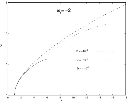
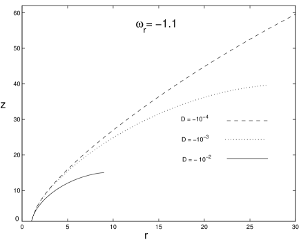
Figure 1: In the figures we show some embedding diagrams $z(r)$ of two-dimensional sections along the equatorial plane ($t=$ const, $\theta=\pi/2$) with the help of Eq. (40) of the traversable evolving wormhole (III). For all diagrams the throat is located at $r_{0}=1$ and curves are drawn for the specified values of $D$ and $\omega_{r}$, taking into account the shape function $b(r)$ of Eq (IV.2). The range of $r$ is $r_{0}<r<r_{max}$, where $r_{max}$ is given by Eq. (43). For a full visualization of the surfaces the diagrams must be rotated about the vertical $z$ axis.

(v) The shape of a wormhole is determined by $b(r)$ as viewed, for example, in an embedding diagram in a flat $3$–dimensional Euclidean space $R^{3}$. To construct such a diagram of a wormhole, one considers an equatorial slice ($\theta=\pi/2$) at a fixed instant of time $t=t_{0}$ of the geometry. Since the wormhole (III) evolves in time, each such slice will be different for different values of time. In other words, the shape of the wormhole is determined also by the scale factor $a(t)$. However, it can be shown that the form of the wormhole is preserved with time, by using an embedding procedure. The metric of a such a wormhole slice for $t=t_{0}=$ const is given by

$$ds^{2}=a^{2}(t_{0})\left(\frac{dr^{2}}{1-\frac{b(r)}{r}}+r^{2}d\varphi^{2}\right),$$ (37)

where $b(r)$ is given by the first expression of Eq. (IV.2). One may rewrite this slice by rescaling the radial coordinate as $\bar{r}=a(t_{0})\,r$. Thus the metric (37) may be rewritten in the following form:

$$ds^{2}=\frac{d\bar{r}^{2}}{1-\frac{\bar{b}(\bar{r})}{\bar{r}}}+\bar{r}^{2}d\varphi^{2},$$ (38)

where we have introduced the definition $\bar{b}(\bar{r})=a(t_{0})\,b(r)$. Now, we shall embed this slice in a flat $3$–dimensional Euclidean space $R^{3}$, which we shall write as

$$ds^{2}=d\bar{z}^{2}+d\bar{r}^{2}+\bar{r}^{2}d\varphi^{2}.$$ (39)

Comparing the metrics (38) and (39) we conclude that

$$\frac{d\bar{z}}{d\bar{r}}=\pm\left(\frac{\bar{r}}{\bar{b}}-1\right)^{-1/2}=\pm\left(\frac{r}{b}-1\right)^{-1/2}.$$ (40)

This implies that the evolving wormhole will remain the same size in the $\bar{z},\bar{r},\varphi$ coordinates.

On the other hand, we also conclude that in order to visualize the slice $\theta=\pi/2$, $t=t_{0}$ embedded into the three-dimensional Euclidean space we must require that the shape function $b(r)$ must be positive and be such that $b(r)/r<1$ in order to guarantee that the root $\sqrt{r/b(r)-1}$ be real, as for static wormholes Lemos . In other words we can draw the graph $\bar{z}=\bar{z}(\bar{r})$ only for $b(r)/r<1$ with $b(r)>0$. In this case the embedded two dimensional section has a minimum radius at the throat $r=r_{0}$ and has the maximum upper radius at the mouth ($b=0$) of the wormhole. For larger radii where $b(r)<0$ the embedding process is no longer valid. Notice that in our case the general metric (II.2), with the scale factor and shape function (21) and (IV.2), is well defined even for $b(r)<0$, being this spacetime geodesically complete. Thus the requirement $b(r)>0$ emphases the fact that the importance of the embedding is near the throat of the wormhole. In our case, as we stated above, far from the wormhole mouth the space is asymptotically flat. In principle, if one includes a cosmological constant, the space can be de-Sitter or anti-de Sitter far from the mouth.

Now in order to maintain the shape of the traversable wormhole the flaring out condition must be required, i.e. $d^{2}\bar{r}/d\bar{z}^{2}>0$. So from Eq. (40) we have that

$$\frac{d^{2}\bar{r}}{d\bar{z}^{2}}=\frac{\bar{b}-\bar{b}^{\prime}r}{2\bar{b}^{2}}=\frac{b-b^{\prime}r}{2a(t_{0})b^{2}}>0,$$ (41)

and taking into account the form of the shape function from Eq. (IV.2) we obtain

$$\frac{d^{2}\bar{r}}{d\bar{z}^{2}}=-\left(\frac{r}{r_{0}}\right)^{1/\omega_{r}}\times\,\,\,\,\,\,\,\,\,\,\,\,\,\,\,\,\,\,\,\,\,\,\,\,\,\,\,\,\,\,\,\,\,\,\,\,\,\,\,\,$$

$$\frac{2D\omega_{r}r^{3}(r/r_{0})^{1/\omega_{r}}+(1+\omega_{r})r_{0}(Dr_{0}^{2}-1)}{2\omega_{r}(Dr^{3}(r/r_{0})^{1/\omega_{r}}+r_{0}(1-Dr_{0}^{2}))^{2}},$$ (42)

which for $D<0$ is always positive, thus satisfying the flaring out condition for the entire range of the radial coordinate $r$. So, as we have seen, a distribution of an anisotropic phantom energy provides the flare-out conditions for the throat of evolving wormholes.

(vi) Let us now study the range of validity of the radial coordinate more adequately. From the condition $b(r)\geq 0$, which we must impose in order to have a good embedding, we obtain that $b(r)=0$ for

$$r_{max}=r_{0}\left(1-\frac{1}{Dr_{0}^{2}}\right)^{\omega_{r}/(1+3\omega_{r})},$$ (43)

implying that $b(r)\geq 0$ for $r\leq r_{max}$. Thus the wormhole is located at the range $r_{0}\leq r\leq r_{max}$, being the throat at $r_{0}$. Notice that the radius $r_{max}$ may be made arbitrarily large by taking $D\rightarrow-0$, but still having an evolving wormhole.

(vii) In order for this evolving wormhole to be traversable, the tidal forces experienced by a traveller must not be too great. So a traveller should feel during its radial journey a tidal acceleration, between two parts of her body (i.e. head to feet), which must not exceed by much one Earth gravity. This traversability criteria was considered in Ref. Morris . In general the tidal acceleration may be written as (the Greek indices take the values $0,1,2,3$)

$$\bigtriangleup a^{\hat{\alpha}}=-c^{2}R^{\hat{\alpha}}_{\,\,\,\,\,\hat{\beta}\hat{\gamma}\hat{\delta}}u^{\hat{\beta}}\xi^{\hat{\gamma}}u^{\hat{\delta}},$$ (44)

where the vector $\xi^{\hat{\gamma}}$ denotes the separation between the head and feet of the traveller’s body, so $\xi^{\hat{\gamma}}$ is a spacelike vector.

In order to calculate the tidal acceleration felt by a traveller we introduce the orthonormal reference frame used by her: $(e_{\hat{0}^{\prime}},e_{\hat{1}^{\prime}},e_{\hat{2}^{\prime}},e_{\hat{3}^{\prime}})$. Since in this frame we have that $\xi^{\hat{0}^{\prime}}=0$ and $u^{\hat{\beta}^{\prime}}=\delta^{\hat{\beta}^{\prime}}_{\hat{0}^{\prime}}$ for the four velocity, and additionally the Riemann tensor is antisymmetric in its first two indices, the tidal acceleration is purely spatial with components (the Latin indices take the values $1,2,3$)

$$\bigtriangleup a^{\hat{k}^{\prime}}=-c^{2}R^{\hat{k}^{\prime}}_{\,\,\,\,\,\hat{0}^{\prime}\hat{j}^{\prime}\hat{0}^{\prime}}\xi^{\hat{j}^{\prime}},$$ (45)

where the spacelike vector $\xi$ may be oriented along any spatial direction in the traveller’s frame.

Now, this traveller moves at a constant speed $v$ with respect to the observer who uses the orthonormal basis (III) and who always remains at rest at constant $r$, $\theta$, $\varphi$. Thus both sets of orthonormal basis vectors are connected by the standard special relativity Lorentz transformation as follows Morris :

$$e_{\hat{0}^{\prime}}=\bar{u}=\gamma e_{\hat{t}}\mp\gamma\beta e_{\hat{r}},$$

$$e_{\hat{1}^{\prime}}=\gamma\beta e_{\hat{r}}\mp\gamma e_{\hat{r}},\,\,\,\,\,\,\,\,\,\,\,\,$$

$$e_{\hat{2}^{\prime}}=e_{\hat{\theta}},e_{\hat{3}^{\prime}}=e_{\hat{\varphi}},\,\,\,\,\,\,\,\,\,\,\,\,\,\,$$ (46)

where $\bar{u}$ is the traveller’s four velocity, $\gamma=(1-\beta^{2})^{-1/2}$, and $\beta=v/c$. In this case the vector $e_{\hat{1}}$ points along the direction of travel (towards increasing radial proper distance $l$).

Thus, from the generic metric (II.2) (with $\Phi(t,r)=0$) and the Lorentz transformation (IV.2), the relevant Riemann tensor components for (45) are

$$R_{{\hat{1}^{\prime}}\hat{0}^{\prime}\hat{1}^{\prime}\hat{0}}=R_{{(r)}(t)(r)(t)}=\frac{\ddot{a}}{a},$$

$$R_{{\hat{2}^{\prime}}\hat{0}^{\prime}\hat{2}^{\prime}\hat{0}^{\prime}}=R_{{\hat{3}^{\prime}}\hat{0}^{\prime}\hat{3}^{\prime}\hat{0}^{\prime}}=\gamma^{2}R_{(\theta)(t)(\theta)(t)}\mp$$

$$2\gamma^{2}\beta R_{(\theta)(t)(\theta)(r)}+\gamma^{2}\beta^{2}R_{(\theta)(r)(\theta)(r)}=$$

$$\gamma^{2}\frac{\ddot{a}}{a}-\frac{\gamma^{2}\beta^{2}}{2a^{2}r^{3}}\left(2\dot{a}^{2}r^{3}-b+rb^{\prime}\right).$$ (47)

If now we consider the size of the traveller’s body to be $|\xi|\sim 2$ (m) and $\mid\bigtriangleup a\mid\leq g_{\oplus}$ ($\equiv$ one Earth gravity, i.e. $9,8$ m$/s^{2}$) the Riemann tensor components are constrained to be

$$|R_{{\hat{1}^{\prime}}\hat{0}^{\prime}\hat{1}^{\prime}\hat{0}}|=\left|\frac{\ddot{a}}{a}\right|\leq\frac{g_{\oplus}}{c^{2}\times 2\,m}\simeq\frac{1}{(10^{8}m)^{2}},$$ (48)

and

$$|R_{{\hat{2}^{\prime}}\hat{0}^{\prime}\hat{2}^{\prime}\hat{0}^{\prime}}|=|R_{{\hat{3}^{\prime}}\hat{0}^{\prime}\hat{3}^{\prime}\hat{0}^{\prime}}|=$$

$$\left|\gamma^{2}\frac{\ddot{a}}{a}-\frac{\gamma^{2}\beta^{2}}{2a^{2}r^{3}}\left(2\dot{a}^{2}r^{3}-b+rb^{\prime}\right)\right|\leq$$

$$\frac{g_{\oplus}}{c^{2}\times 2\,m}\simeq\frac{1}{(10^{8}m)^{2}}.$$

Notice that, since the wormhole metric evolves with time, the tidal acceleration also depends on time. In this case the radial tidal constraint (48) can be regarded as directly constraining the acceleration of the expansion of the wormhole, while the lateral tidal constraint (IV.2) can be regarded as constraining the speed $v$ of the traveller while crossing the wormhole.

$v_{max}$	$\omega_{r}$	$r_{0}$
$542$ m/s	$-1.5$	$100$ m
$1038$ m/s	$-1.1$	$100$ m
$1084$ m/s	$-1.5$	$200$ m
$2076$ m/s	$-1.1$	$200$ m

Table 1: This table shows the maximum values of $v_{max}$ at which the traveller could cross the static wormhole for given values of $\omega_{r}$ and $r_{0}$ in order to satisfy the constraint on the lateral tidal acceleration.

$t_{min}$	$D$	$v$	$\omega_{r}$	$r_{0}$
$4.55$ s	$-15$	$50$ m/s	$-1.1$	$100$ m
$1.65$ s	$-0.1$	$50$ m/s	$-1.1$	$100$ m
$4.55$ s	$-15$	$50$ m/s	$-1.1$	$200$ m
$1.65$ s	$-0.1$	$50$ m/s	$-1.1$	$200$ m
$6.06$ s	$-0.1$	$50$ m/s	$-1.5$	$100$ m
$4.71$ s	$-100$	$50$ m/s	$-1.1$	$100$ m

Table 2: This table shows the minimum values $t_{mim}$ for the cosmological time at which the traveller could cross the evolving wormhole for given values of $D$ ($F=1$), $v$, $\omega_{r}$ and $r_{0}$ in order to saturate the constraint on the lateral tidal acceleration.

In particular, the evolving wormholes obtained in this paper evolve with the scale factor (21). This implies that the expansion is not accelerated (i.e. $\ddot{a}=0$) and then the radial tidal acceleration is identically zero, thus satisfying the constraint (48). On the other hand, by taking into account Eqs. (III) and (IV.2) we obtain the following constraint for the lateral tidal acceleration:

$$\left|\gamma^{2}\beta^{2}\frac{\kappa C(1+\omega_{r})\,r^{-(1+3\omega_{r})/\omega_{r}}}{2(\sqrt{-D}t+F)^{2}}\right|\leq\frac{g_{\oplus}}{c^{2}\times 2\,m}\simeq$$

$$\frac{1}{(10^{10}cm)^{2}}.$$ (50)

It is interesting to note that the lateral tidal acceleration at fixed $r$ diminishes with time. Now by taking into account Eq. (22) this constraint may be rewritten as

$$\left|\frac{1}{2}\,\gamma^{2}\beta^{2}\kappa(1+\omega_{r})\rho\right|\lesssim\frac{1}{(10^{10}cm)^{2}},$$ (51)

thus the lateral tidal constraint (IV.2) can be regarded more exactly as constraining both the speed $v$ of the traveller and the energy density of the matter threading the wormhole. By taking into account the expression for the energy density of Eq. (IV.2) and considering that the motion of the traveller is nonrelativistic ($v<<c$, $\gamma\approx 1$) we may rewrite Eq. (51) as follows:

$$\left|\frac{v^{2}(1+\omega_{r})(1-Dr_{0}^{2})}{\omega_{r}r_{0}^{2}(\sqrt{-D}t+F)^{2}}\right|\lesssim g_{\oplus}.$$ (52)

For the static case (i.e. $D=0$ and $F=1$) Eq. (52) gives the following constraint on the speed $v$:

$$v\lesssim\sqrt{\frac{g_{\oplus}\,\omega_{r}\,r_{0}^{2}}{1+\omega_{r}}}.$$ (53)

In Table 1 we show the maximum values of the speed at which the traveller could cross the static wormhole for some given values of the $\omega_{r}$ and $r_{0}$ parameters in order to satisfy the constraint (53).

In table 2 we show for some given values of $\omega_{r}$, $r_{0}$, $D$ ($F=1$) and $v$ the minimum values of the cosmological time $t=t_{min}$ at which it is possible to cross the evolving wormhole in order to satisfy the constraint (52) for $t\geq t_{min}$.

(viii) This wormhole solution also may be interpreted as an interior one Arellano . This implies that one may, in principle, match the found wormholes to an exterior Kottler solution (Schwarzschild–de Sitter or Schwarzschild–anti de Sitter spacetimes) at some matching interface $r_{m}$, where $r_{0}<r_{m}<r_{max}$ (see Fig. 1), in the spirit of made in Ref. Lemos , where a procedure is given for matching static spherically symmetric wormholes to Kottler solution by using directly the field equations to make the match. This work is in progress.

V Conclusions

In this paper we have constructed exact evolving wormhole geometries supported by phantom energy, showing explicitly that the phantom energy can support the existence of evolving wormholes. Specifically we have constructed asymptotically flat evolving wormholes with radial and tangential pressures obeying barotropic equations of state with constant state parameters. One interesting feature of these evolving wormholes, supported by an anisotropic phantom matter, is that they expand with constant velocity.

VI Acknowledgements

This work was supported by CONICYT through Grants FONDECYT N⁰ 1080530 and 1070306 (MC, SdC and PS), and by Dirección de Investigación de la Universidad del Bío–Bío (MC and PL). SdC also was supported by PUCV grant N⁰ 123.787/2008. P.S. and J.C. were supported by Universidad de Concepción through DIUC Grants N⁰ 208.011.048-1.0 and 205.011.038-1 respectively.

References

- (1) S. Coleman, Nucl Phys. 307, 867 (1988).
- (2) S.B. Giddings and A. Strominger, Nucl. Phys. B 321, 481 (1988).
- (3) M.S. Morris and K.S. Thorne, Am. J. Phys. 56, 395 (1988); M.S. Morris, K.S. Thorne and U. Yurtsever, Phys. Rev. Lett. 61, 1446 (1988).
- (4) J.D. Novikov, Sov. Phys. JETP 68, 439 (1989).
- (5) M. Visser, Lorentzian Wormholes: From Einstein to Hawking, (AIP, New York, 1995); M. Visser, S. Kar, N. Dadhich Phys. Rev. Lett. 90 201102 (2003); N. Dadhich, S. Kar, S. Mukherjee and M. Visser, Phys. Rev. D 65, 064004 (2002).
- (6) E. Teo, Phys. Rev. D 58, 024014 (1998); V.M. Khatsymovsky, Phys. Lett. B 429, 254 (1998); P. K. F. Kuhfittig, Phys. Rev. D 67, 064015 (2003); Tonatiuh Matos, D. Nunez Class. Quant. Grav. 23, 4485 (2006); Mubasher Jamil, Muneer Ahmad Rashid, Electromagnetic field around a slowly rotating wormhole arXiv: 0805.0966 [astro-ph].
- (7) S. Kar, Phys. Rev. D 49, 862 (1994).
- (8) S. Kar and D. Sahdev, Phys. Rev. D 53, 722 (1996).
- (9) F.S.N. Lobo, Exotic solutions in General Relativity: Traversable wormholes and ’warp drive’ spacetimes, e-Print: arXiv:0710.4474 [gr-qc]; A. V. B. Arellano and F. S. N. Lobo; Class. Quant. Grav. 23, 5811 (2006).
- (10) A. V. B. Arellano and F. S. N. Lobo; Class. Quant. Grav. 23, 7229 (2006).
- (11) G.P. Perry and R.B. Mann, Gen. Rel. Grav. 24, 305 (1992); S.W. Kim, H.J. Lee, S.K. Kim and J.M. Yang, Phys. Lett. A 183, 359 (1993); M.S.R. Delgaty and R.B. Mann, Int. J. Mod. Phys. D 4, 231 (1995); Y.G. Shen and Z.Q. Tan, Annals Phys. 272, 1 (1999); W.T. Kim, E.J. Son and M.S. Yoon, Phys. Rev. D 70, 104020 (2004); W.T. Kim, J.J. Oh and M.S. Yoon, Phys. Rev. D 70, 044006 (2004).
- (12) P. Gonzales–Diaz, Phys. Lett. B 247, 251 (1990); X. Jianjun and J. Sicong, Mod. Phys. Lett. 6, 251 (1990).
- (13) Gerard Clement, Gen. Rel. Grav. 16, 131, (1984.); M. Cataldo, P. Salgado and P. Minning, Phys. Rev. D 66, 124008 (2002).
- (14) B. Bhawal and S. Kar, Phys. Rev. D 46, 2464 (1992); G. Dotti, J. Oliva, R. Troncoso, Phys. Rev. D 76, 064038 (2007); G. Dotti, J. Oliva, R. Troncoso, Phys. Rev. D 75, 024002 (2007).
- (15) S. Kar and D. Sahdev, Phys. Rev. D 53, 722 (1996); A. DeBenedictis and D. Das, Nucl. Phys. B 653, 279 (2003).
- (16) C. Barcelo, L. J. Garay, P. F. Gonzalez-Diaz and G. A. Mena Marugan, Phys. Rev. D 53, 3162 (1996).
- (17) T.A. Roman, Phys. Rev. D 47, 1370 (1993).
- (18) S. Nojiri, S. D. Odintsov and S. Tsujikawa, Phys. Rev. D 71, 063004 (2005); P. F. Gonzalez-Diaz, Phys. Rev. D 68, 021303 (2003); P. F. Gonzalez-Diaz, Phys. Lett. B 586, 1 (2004); M. Cataldo, N. Cruz and S. Lepe, Phys. Lett. B 619, 5 (2005); G. Izquierdo and D. Pavon, Phys. Lett. B 633, 420 (2006).
- (19) S. V. Sushkov, Phys. Rev. D 71, 043520 (2005)
- (20) F. S. N. Lobo, Phys. Rev. D 71, 084011 (2005); F.S.N. Lobo, gr-qc/0603091; P. K. F. Kuhfittig, Class. Quant. Grav. 23, 5853 (2006).
- (21) M. Visser and C. Barcelo, Energy conditions and their cosmological implications, gr-qc/0001099.
- (22) J. P. S. Lemos, F. S. N. Lobo and S. Quinet de Oliveira, Phys. Rev. D 68, 064004 (2003).