Diffusion of two particles with a finite interaction potential in one dimension

Abstract

We investigate the dynamics of two interacting diffusing particles in an infinite effectively one dimensional system; the particles interact through a step-like potential of width $b$ and height $\phi_{0}$ and are allowed to pass one another. By solving the corresponding 2+1-variate Fokker-Planck equation an exact result for the two particle conditional probability density function (PDF) is obtained for arbitrary initial particle positions. From the two-particle PDF we obtain the overtake probability, i.e. the probability that the two particles has exchanged positions at time $t$ compared to the initial configuration. In addition, we calculate the trapping probability, i.e. the probability that the two particles are trapped close to each other (within the barrier width $b$) at time $t$, which is mainly of interest for an attractive potential, $\phi_{0}<0$. We also investigate the tagged particle PDF, relevant for describing the dynamics of one particle which is fluorescently labeled. Our analytic results are in excellent agreement with the results of stochastic simulations, which are performed using the Gillespie algorithm.

I Introduction

As recent advances in manufacturing methods drives device sizes toward the nanorange, the understanding of how interactions between diffusing entities affect dynamics is becoming increasingly important CD . Situations where diffusing molecules interact strongly are also of importance in biological systems Ellis .

The interaction between diffusing particles can be of either attractive or repulsive nature. For repulsive interactions, a particularly prominent example is that of single-file diffusion, i.e. the diffusion of identical particles which interact via a hardcore repulsion (the interaction potential energy is plus infinity, so that the particles cannot pass each other) in one dimension. For single-filing systems the particle order is thus conserved over time $(t)$ resulting in interesting dynamical behavior for a tagged particle. For instance, in contrast to ordinary diffusion for which the mean square displacement $\langle(x_{\cal T}-x_{{\cal T},0})^{2}\rangle$ is proportional to $t$, for single file diffusion the mean square displacement of a tagged particle is proportional square root of time, $\langle(x_{\cal T}-x_{{\cal T},0})^{2}\rangle\propto t^{1/2}$ for long times in an infinite system with a fix particle concentration HA ; Alexander_Pincus_78 ; WBL ; the probability density function (PDF) the single-file of the tagged particle position is Gaussian HA ; LE ; Beijeren_83 ; Hahn_95 ; RKH ; Kollmann_03 ; Jara_Landim_06 ; Lizana_Ambjornsson . For attractive interactions an especially well-studied example is that of reaction-diffusion system Evans_02 , where often the particles are assumed to annihilate each other upon encounter, i.e. the potential energy between particles is assumed to be minus infinity.

Although much work has been dedicated to interacting diffusing particles interacting via infinite (negative or positive) potentials, to our knowledge, much fewer studies consider finite potentials. In Ref. Kutner_84, the problem of diffusion of $N$ particles on two coupled linear chains was studied. Similarly, in Refs. Hahn_98, and Mon_02, diffusion of spherical particles in a cylindrical geometry, where the cylinder radius was large enough to allow passage of particles, were studied; in Ref. Hahn_98, molecular dynamics simulations were done using a Lennard Jones interaction between particles and in Ref. Mon_02, a Monte Carlo simulation using a hard sphere interaction was performed. Recently, the dynamics of a tagged particle in a system consisting of particles interacting through screened repulsive Coulomb interactions in one dimension was investigatedNelissen , however only through stochastic simulations. In this study we derive analytic results for diffusing particles interacting through finite potentials: we solve analytically the problem of diffusion of two particles interacting via a finite-sized potential of finite height in one dimension, for arbitrary initial particle positions. Our results generalize the single barrier results of Ref. Berdichevsky, (who solved a similar problem by Laplace transform techniques) to arbitrary initial particle positions.

This paper has the following organization: In Sec. II we state the problem under consideration and formulate the relevant equations. In Sec. III we provide the solution of the equations for the two particle conditional probability density function (PDF). In Sec. IV we use the two particle PDF to obtain the overtake probability, i.e. the probability that the two particles at time $t$ have exchanged positions compared to the initial configuration. In Sec. V we calculate the trapping probability, i.e. the probability that the two particles are trapped close to each other (within the barrier width) at time $t$. In Sec. VI we obtain the PDF for one of the particles being tagged. We compare our analytic results to stochastic simulations using the Gillespie algorithm and find excellent agreement. Finally, in Sec VII we give a summary and outlook.

II Problem definition

We consider a system with two interacting point particles diffusing in an infinite one dimensional system. The point particle problem considered here can be transformed into a problem of finite-sized interacting particles using a similar mapping as given in Ref. Lizana_Ambjornsson, . A cartoon of the system we have in mind is depicted in Fig. 1.

Figure 1: Cartoon of the problem considered in this study: two point particles are diffusing in an infinite one dimension system. Particle $j$ has coordinate $x_{j}$, and initial coordinate $x_{j,0}$ ($j=1,2$). The particles interact via a step-potential of width $b$ and height $\phi_{0}$, see Fig. 2.

The particles have coordinates $\vec{x}=(x_{1},x_{2})$ and initial positions $\vec{x}_{0}=(x_{1,0},x_{2,0})$. We assume that the particles interact through a step-like potential of width $b$ and height $\phi_{0}$, i.e. the potential is

$$\Phi(x_{1},x_{2}) = 0\ {\rm for}\ x_{1}-x_{2}<-b/2\ ({\rm region}\ 12)$$ (1)

$$= \phi_{0}\ {\rm for}\ |x_{1}-x_{2}|<b/2\ ({\rm region}\ 1-2)$$

$$= 0\ {\rm for}\ x_{1}-x_{2}>b/2\ ({\rm region}\ 21).$$

The phase space is depicted in Fig. 2, where the darker area corresponds to the region of non-zero potential. For $\phi_{0}>0$ we have a barrier, whereas for $\phi_{0}<0$ the potential is of a short-range attractive nature.

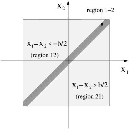
Figure 2: Phase space region for the system, the darker area, $|x_{1}-x_{2}|<b/2$, corresponds to a region where the potential is of height $\phi_{0}$, the potential width is $b$. In the lighter shaded areas the potential is zero. The system is assumed to be infinite, i.e. $-\infty<x_{1},x_{2}<\infty$.

The spatial distribution of the particles as a function of time is contained in the two particle conditional PDF ${\cal P}(\vec{x},t|\vec{x}_{0})$, which gives the probability of particle $1$ being in the interval $[x_{1},x_{1}+dx_{1}]$ and particle $2$ in $[x_{2},x_{2}+dx_{2}]$ at time $t$ given that they initially (at time $t=0$) were at positions $x_{10}$ and $x_{2,0}$ respectively. Since inside each of the three regions the potential energy landscape is flat (the force is zero) this quantity is governed by the $2+1$ (two coordinates and time) variable Fokker-Planck (Smoluchowski) equation

$$\frac{\partial{\cal P}_{\gamma}(\vec{x},t|\vec{x}_{0})}{\partial t}=D\left(\frac{\partial^{2}}{\partial x_{1}^{2}}+\frac{\partial^{2}}{\partial x_{2}^{2}}\right){\cal P}_{\gamma}(\vec{x},t|\vec{x}_{0}),$$ (2)

where $\gamma=12,1-2$ and $21$ indicates phase-space regions, and $D$ is the diffusion constant for the particles. At the boundaries between regions we have the following conditions Risken ; Risken2

$${\rm flux}\ J\ {\rm continuous}\ {\rm at}\ |x_{1}-x_{2}|=b/2$$

$$\exp(-\beta\Phi(\vec{x})){\cal P}_{\gamma}(\vec{x},t|\vec{x}_{0})\ {\rm continuous}\ {\rm at}\ |x_{1}-x_{2}|=b/2,$$ (3)

where $\beta=1/(k_{B}T)$, and $k_{B}$ is the Boltzmann constant and $T$ the temperature. We assume that the particles start in region $12$ initially, i.e particle $1$ starts to the left of particle $2$. The initial condition then becomes:

$${\cal P}_{12}(\vec{x},t\rightarrow 0|\vec{x}_{0}) = \delta(x_{1}-x_{1,0})\delta(x_{2}-x_{2,0}),$$

$${\cal P}_{1-2}(\vec{x},t\rightarrow 0|\vec{x}_{0}) = {\cal P}_{21}(\vec{x},t\rightarrow 0|\vec{x}_{0})=0,$$ (4)

where $\delta(z)$ denotes the Dirac delta-function.

III Two-particle probability density function

In order to solve the equations specified in the previous section we make a variable transformation to the center-of-mass position $X$ and relative coordinate $s$ according to:

$$X = \frac{1}{2}\left(x_{1}+x_{2}\right),$$

$$s = x_{1}-x_{2}.$$ (5)

Eqs. (2) and (II) then becomes (leaving the argument corresponding to the initial positions implicit)

$$\frac{\partial{\cal P}_{\gamma}(X,s,t)}{\partial t} = \left(D^{X}\frac{\partial^{2}}{\partial X^{2}}+D^{s}\frac{\partial^{2}}{\partial s^{2}}\right){\cal P}_{\gamma}(X,s,t),$$

$${\cal P}_{12}(X,s,t\rightarrow 0) = \delta(X-X_{0})\delta(s-s_{0}),$$

$${\cal P}_{1-2}(X,s,t\rightarrow 0) = {\cal P}_{21}(X,s,t\rightarrow 0)=0,$$ (6)

where $X_{0}=(x_{1,0}+x_{2,0})/2$ and $s_{0}=x_{1,0}-x_{2,0}$ ($s_{0}<-b/2$) and the effective diffusion constants

$$D^{X} = \frac{D}{2},$$

$$D^{s} = 2D.$$ (7)

The equations above express the fact that the relative coordinate $s$ diffuses with a diffusion constant $2D$, whereas the center-of-mass coordinate $X$ diffuses with a diffusion constant $D/2$. The boundary conditions, Eqs. (II), give rise to the four equations:

$$\frac{\partial{\cal P}_{12}(X,s,t)}{\partial s}|_{s=-b/2} = \frac{\partial{\cal P}_{1-2}(X,s,t)}{\partial s}|_{s=-b/2},$$

$$\frac{\partial{\cal P}_{1-2}(X,s,t)}{\partial s}|_{s=b/2} = \frac{\partial{\cal P}_{21}(X,s,t)}{\partial s}|_{s=b/2},$$ (8)

which expresses the continuity of flux and

$${\cal P}_{12}(X,s=-b/2,t)=\exp(\frac{\phi_{0}}{k_{B}T}){\cal P}_{1-2}(X,s=-b/2,t),$$

$$\exp(\frac{\phi_{0}}{k_{B}T}){\cal P}_{1-2}(X,s=b/2,t)={\cal P}_{21}(X,s=b/2,t),$$ (9)

which corresponds to a detailed balance-like condition van_Kampen at the boundaries. The boundary conditions above are different from the corresponding problem in quantum mechanics CohenTannoudji where the wavefunction and the derivative of the wavefunction are continuous - the origin of this difference is due to the fact that in the quantum mechanical problem the potential enters in the equation of motion (the Schrödinger equation), whereas in the Fokker-Planck equation it is the force which enters.

Eqs. (III), (III) and (III) allow a product solution of the form

$${\cal P}_{\gamma}(X,s,t)={\cal P}^{X}(X,t){\cal P}_{\gamma}^{s}(s,t),$$ (10)

where (the boundary conditions involve only the relative coordinate $s$)

$${\cal P}^{X}(X,t)=\frac{1}{(4\pi D^{X}t)^{1/2}}\exp(-\frac{(X-X_{0})^{2}}{4D^{X}t}).$$ (11)

For the solution for ${\cal P}_{\gamma}^{s}(s,t)$ we take a general function that satisfies the diffusion equation in each of the regions and that satisfies the boundary conditions:

$${\cal P}^{s}(s,t)=\int_{-\infty}^{\infty}\frac{dQ}{2\pi}e^{-E(Q)t}e^{-iQs_{0}} \times [C_{12}^{+}e^{iQs}+C_{12}^{-}e^{-iQs}]\ {\rm for}\ s<-b/2$$ (12)

$$\times [C_{1-2}^{+}e^{iQs}+C_{1-2}^{-}e^{-iQs}]\ {\rm for}\ |s|<b/2$$

$$\times C_{21}^{+}e^{iQs}\ {\rm for}\ s>b/2.$$

The prefactors $C^{\pm}_{\gamma}$ are dependent on Q in general. Inserting Eq. (12) into the equation of motion [see Eq. (III)] gives the dispersion relation:

$$E(Q)=D^{s}Q^{2}.$$ (13)

We proceed by setting $C_{12}^{+}=1$ (we will show that with this choice the initial condition is satisfied). Inserting Eq. (12) into the boundary conditions Eqs. (III) and (III) produces 4 equations for the four unknowns $C_{12}^{-}$, $C_{1-2}^{+}$ and $C_{1-2}^{-}$ and $C_{21}^{+}$. Solving this set of equations gives:

$$C_{12}^{-}(Q) = F\frac{1}{1-F^{2}e^{2iQb}}[e^{-iQb}-e^{iQb}],$$

$$C_{1-2}^{+}(Q) = (1-F)\frac{1}{1-F^{2}e^{2iQb}},$$

$$C_{1-2}^{-}(Q) = -F(1-F)\frac{1}{1-F^{2}e^{2iQb}}e^{iQb},$$

$$C_{21}^{+}(Q) = (1+F)(1-F)\frac{1}{1-F^{2}e^{2iQb}},$$ (14)

where we introduced an effective “reflection” coefficient

$$F=\frac{e^{\beta\phi_{0}}-1}{e^{\beta\phi_{0}}+1}=\tanh[\frac{\beta\phi_{0}}{2}].$$ (15)

Notice that for the case of a barrier-like potential, $\phi_{0}\geq 0$, we have $0\leq F<1$, where $F=0$ corresponds to the absence of the barrier and $F\rightarrow 1$ corresponds to an infinite barrier. For the case of an attractive potential, $\phi_{0}<0$, we have $-1<F<0$, where $F\rightarrow-1$ corresponds to an infinite potential well. Combining Eq. (12), (13) and (III) we have:

$${\cal P}_{12}^{s}(s,t) = \Psi(s-s_{0},t)+F\{\Upsilon(-[s+s_{0}+b],t)-\Upsilon(-[s+s_{0}-b],t)\},$$

$${\cal P}_{1-2}^{s}(s,t) = (1-F)\Upsilon(s-s_{0},t)-F(1-F)\Upsilon(-[s+s_{0}-b],t),$$

$${\cal P}_{21}^{s}(s,t) = (1-F^{2})\Upsilon(s-s_{0},t),$$ (16)

where

$$\Psi(\alpha,t)=\int_{-\infty}^{\infty}\frac{dQ}{2\pi}e^{-D^{s}Q^{2}t}e^{i\alpha Q}=\frac{1}{(4\pi D^{s}t)^{1/2}}\exp\large(-\frac{\alpha^{2}}{4D^{s}t}\large)$$ (17)

and

$$\Upsilon(\alpha,t)=\int_{-\infty}^{\infty}\frac{dQ}{2\pi}\frac{1}{1-F^{2}e^{2iQb}}e^{-D^{s}Q^{2}t}e^{i\alpha Q}.$$ (18)

The above expression for $\Upsilon(\alpha,t)$ can be explicitly evaluated: using $1/(1-z)=\sum_{n=0}^{\infty}z^{n}$ (valid for $|z|<1$) we have

$$\Upsilon(\alpha,t) = \int_{-\infty}^{\infty}\frac{dQ}{2\pi}\sum_{n=0}^{\infty}F^{2n}e^{-D^{s}Q^{2}t}e^{i\alpha Q(\alpha+2bn)}$$ (19)

$$= \sum_{n=0}^{\infty}F^{2n}\frac{1}{(4\pi D^{s}t)^{1/2}}\exp\large(-\frac{(\alpha+2bn)^{2}}{4D^{s}t}\large).$$

i.e. $\Upsilon(\alpha,t)$ is a sum of shifted Gaussians weighted by powers of the reflection coefficient $F$ [see Eq. (15)]. The full solution to the problem is specified by Eqs. (10) (11), (III), (17) and (19), where $X$ and $s$ are related to $x_{1}$ and $x_{2}$ using Eq. (III). Finally, returning to our original coordinates we find that the two-particle conditional PDF becomes:

$${\cal P}_{12}(\vec{x},t|\vec{x}_{0}) = Q(x_{1}-x_{1,0})Q(x_{2}-x_{2,0})$$

$$+F\sum_{n=0}^{\infty}F^{2n}\{Q(x_{1}-x_{2,0}+\frac{b}{2}-bn)Q(x_{2}-x_{1,0}-\frac{b}{2}+bn)$$

$$\hskip 42.67912pt-Q(x_{1}-x_{2,0}-\frac{b}{2}-bn)Q(x_{2}-x_{1,0}+\frac{b}{2}+bn)\}$$

$${\cal P}_{1-2}(\vec{x},t|\vec{x}_{0}) = (1-F)\sum_{n=0}^{\infty}F^{2n}\{Q(x_{1}-x_{1,0}+bn)Q(x_{2}-x_{2,0}-bn)$$

$$\hskip 42.67912pt-FQ(x_{1}-x_{2,0}-\frac{b}{2}-bn)Q(x_{2}-x_{1,0}+\frac{b}{2}+bn)\}$$

$${\cal P}_{21}(\vec{x},t|\vec{x}_{0}) = (1-F^{2})\sum_{n=0}^{\infty}F^{2n}Q(x_{1}-x_{1,0}+bn)Q(x_{2}-x_{2,0}-bn),$$ (20)

where

$$Q(\alpha)=\frac{1}{(4\pi Dt)^{1/2}}\exp(\frac{-\alpha^{2}}{4Dt}).$$ (21)

It is a straightforward matter to show, using $\delta(x-a)={\rm lim}_{t\rightarrow 0}\exp[-(x-a)^{2}/(4Dt)]/\sqrt{4\pi Dt}$, that the result above satisfies the initial condition specified in Eq. (III) [and that, therefore, indeed taking $C^{+}_{12}=1$ was the correct choice]. In the absence of a barrier, $F\rightarrow 0$, we find ${\cal P}(x_{1},x_{2},t)=Q(x_{1}-x_{1,0})Q(x_{2}-x_{2,0})$ as it should. For the case of an infinite barrier, $F\rightarrow 1$, we have: ${\cal P}_{12}(x_{1},x_{2},t)=Q(x_{1}-x_{1,0})Q(x_{2}-x_{2,0})+Q(x_{1}-x_{2,0}+b/2)Q(x_{2}-x_{1,0}-b/2)$ and ${\cal P}_{1-2}(x_{1},x_{2},t)={\cal P}_{21}(x_{1},x_{2},t)=0$ in agreement with the result for hardcore interacting particles of linear size $b/2$. Lizana_Ambjornsson For the case of an infinite potential well $F\rightarrow-1$, the solution for region 12 takes the form: ${\cal P}_{12}(x_{1},x_{2},t)=Q(x_{1}-x_{1,0})Q(x_{2}-x_{2,0})-Q(x_{1}-x_{2,0}+b/2)Q(x_{2}-x_{1,0}-b/2)$; this result agrees with previous results for two vicious walkers (the random walkers kill each other upon encounter). Fisher_84 ; Novotny

IV Overtake probability

In this section we calculate the overtake probability ${\cal}W(t)$, i.e. the probability that particle 1 is to the right of particle 2 at time $t$. We have:

$${\cal}W(t)=\int dx_{1}\int dx_{2}|_{{\rm region}\ 21}{\cal P}(x_{1},x_{2},t).$$ (22)

Changing coordinates to $X$ and $s$, see Eq. (III), we get

$${\cal}W(t) = \int_{-\infty}^{\infty}dX{\cal P}^{X}(X,t)\int_{b/2}^{\infty}ds{\cal P}_{21}^{s}(s,t)$$ (23)

$$= \frac{1}{2}(1-F^{2})\sum_{n=0}^{\infty}F^{2n}{\rm erfc}[\frac{b(2n+1/2)-s_{0}}{\sqrt{4D^{s}t}}],$$

where ${\rm erfc}(z)=1-{\rm erf}(z)$ is the complementary error function, ${\rm erf}(z)=(2/\sqrt{\pi})\int_{0}^{z}dy\exp(-y^{2})$ is the error function ABST , and $s_{0}=x_{1,0}-x_{2,0}$ as before. We have above used the fact that $\int_{-\infty}^{\infty}dX{\cal P}^{X}(X,t)=1$ [see Eqs. (11)] together with Eqs. (10), (III), (17) and (19). The result given in Eq. (23) agrees with the result derived in Ref. Berdichevsky, (using a Laplace-space formalism), where the problem of passage of one particle (since the center-of-mass coordinate is integrated out above, ${\cal}W(t)$ is effectively a one-dimensional quantity) across one and two barriers in finite and infinite one dimensional systems were considered - however in Ref. Berdichevsky, the initial position were taken to be right at the left border (i.e. $s_{0}=-b/2$), the result given in Eq. (23) thus generalizes the one barrier (infinite system) result in Ref. Berdichevsky, to general initial condition. We point out that ( $\phi_{0}\leftrightarrow-\phi_{0}$ is equivalent to $F\leftrightarrow-F$) since ${\cal}W(t)$ contain only even powers of $F$ the overtake probability is invariant under the reversal of sign of the potential $\phi_{0}\leftrightarrow-\phi_{0}$; it thus takes equally long times to pass a barrier of height $\phi_{0}$ as it takes to pass a trap of height $-\phi_{0}$. Using the fact that ${\rm erfc}(0)=1$ we find that for long times $t\rightarrow\infty$ we have $W(t)\rightarrow 1/2$ as it should.

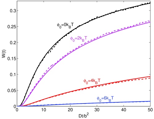
Figure 3: Overtake probability ${\cal}W(t)$ as a function of time $t$ for different barrier heights $\phi_{0}$. The solid curves are the analytic result, Eq. (23), and the dashed curves are the results of stochastic simulations. The following parameters were used $x_{1,0}=-3b$, $x_{2,0}=3b$, where $b$ is the barrier width. The simulation was performed using the Gillespie algorithm on a lattice with $M=5000$ lattice sites, averaged over $n=10000$ ensembles, and with a lattice spacing $a=0.025b$.

In Fig. 3 we illustrate the overtake probability as given in Eq. (23). We notice that an increased potential height leads to decreased probability for overtaking. Also, due to the time it takes for the particles to approach each other through diffusion, there is an initial time $\tau_{c}$ before the probability of overtaking becomes appreciable (even for zero potential); a simple estimate gives $\tau_{c}\sim(x_{2,0}-x_{1,0}-b)^{2}/(2D^{s})$. In Fig. 3 we also compare the analytic results to that of a stochastic simulation using the Gillespie algorithm (see Appendix A), and find excellent agreement.

V Trapping probability

In this section we calculate the trapping probability ${\cal T}(t)$, i.e. the probability that the two particles are at a distance closer than $b$ to each other at time $t$. We have

$${\cal T}(t)=\int dx_{1}\int dx_{2}|_{{\rm region}\ 1-2}{\cal P}(x_{1},x_{2},t).$$ (24)

Again, changing coordinates to $X$ and $s$, see Eq. (III), we have

$${\cal T}(t) = \int_{-\infty}^{\infty}dX{\cal P}^{X}(X,t)\int_{-b/2}^{b/2}ds{\cal P}_{1-2}^{s}(s,t),$$ (25)

$$= \frac{(1-F)}{2}\sum_{n=0}^{\infty}F^{2n}\{(1+F){\rm erf}[\frac{b(2n+1/2)-s_{0}}{\sqrt{4D^{s}t}}]$$

$$-{\rm erf}[\frac{b(2n-1/2)-s_{0}}{\sqrt{4D^{s}t}}]-F{\rm erf}[\frac{b(2n+3/2)-s_{0}}{\sqrt{4D^{s}t}}]\}.$$

For long times $t\rightarrow\infty$ we have that the trapping probability approaches zero ${\cal T}(t)\rightarrow 0$; this is due to ergodicity [each point in our system is assigned a probability proportional to $\exp(-\beta\phi_{0}$)] combined with the fact that our potential well is of finite width ($=b$) and connected to an infinite system.

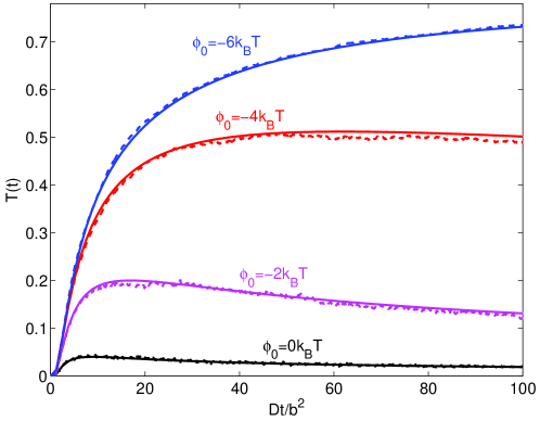
Figure 4: Trapping probability ${\cal T}(t)$ as a function of time $t$ for different potential heights $\phi_{0}$. The solid curves are the analytic result, Eq. (25), and the dashed curves are the results of a stochastic simulation. Except for the differently chosen values for $\phi_{0}$ we used the same parameters as in Fig. 3.

In Fig. 4 we illustrate the trapping probability given by Eq. (25); we find excellent agreement with stochastic simulations. We notice that a more negative potential depth leads to increased probability for trapping as it should. Similarly to the overtake probability, due to the time it takes for the particles to approach each other through diffusion, there is an initial time $\tau_{c}$ before any significant number of trapping events has occurred.

A possible experiment testing the predictions in this section would involve, for instance, two fluorescent molecules; the two molecules interact through a potential and assuming that when the molecules are within some distance $b$ from each other the total fluorescence get quenched or enhanced one could directly detect a binding event between the two particles as an increase or decrease in total fluorescence (fluorescence measurement are here assumed ensemble averaged over thermal noise, with fixed initial particle positions). In such an experiment it may be more convenient to, rather than obtain ${\cal T}(t)$ from experimental data, use time-integrated fluorescences, i.e., measure the time-averaged trapping probability as given by ${\cal T}_{\rm av}(t)=(1/t)\int_{0}^{t}{\cal T}(t^{\prime})dt^{\prime}$. With the help of Eq. (25) we straightforwardly obtain:

$${\cal T}_{\rm av}(t) = \frac{(1-F)}{2}\sum_{n=0}^{\infty}F^{2n}\{(1+F)G(\frac{b(2n+1/2)-s_{0}}{\sqrt{4D^{s}t}})$$ (26)

$$-G(\frac{b(2n-1/2)-s_{0}}{\sqrt{4D^{s}t}})-FG(\frac{b(2n+3/2)-s_{0}}{\sqrt{4D^{s}t}})\}.$$

where we defined a function $G(z)=2z\exp(-z^{2})/\sqrt{\pi}-2z^{2}{\rm erfc}(z)+{\rm erf}(z)$.

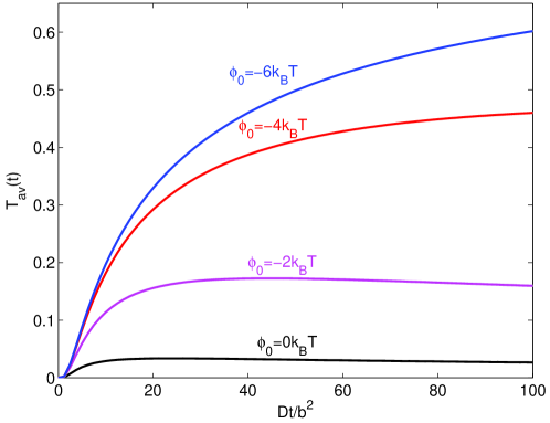
Figure 5: Time-averaged trapping probability ${\cal T}_{\rm av}(t)$ as a function of time $t$ for different potential heights $\phi_{0}$, Eq. (26). Except for the differently chosen values for $\phi_{0}$ we used the same parameters as in Fig. 3.

In Fig. 5 we illustrate the time-averaged trapping probability given by Eq. (26) for different potential heights as a function of $t$. Experimental measurements of ${\cal T}(t)$ or ${\cal T}_{\rm av}(t)$ would provide detailed information about the nature of the interaction potential between the two particles, i.e. of $\phi_{0}$ and $b$, by comparison to our analytic expressions.

Finally, as a simple check of the results in Secs. IV and V, we calculate the first passage time density for two vicious walkers ($F=-1$). The “survival” probability $S(t)$ (i.e. the probability that particle 1 and 2 has not met at time $t$) is given by $S(t)=1-W(t)-T(t)$, which for $F=-1$ becomes $S(t)={\rm erf}[-(s_{0}+b/2)/\sqrt{4D^{s}t}]$, using Eqs. (23) and (25). The first passage time density is then $-dS(t)/dt=[|s_{0}+b/2|/\sqrt{4\pi D^{s}}]t^{-3/2}\exp[-(s_{0}+b/2)^{2}/(4D^{s}t)]$, which agrees with the standard result van_Kampen for the first passage time problem for a diffusing particle (diffusion constant $D^{s}$) starting a distance $s_{0}+b/2$ from a perfectly absorbing wall, as it should.

VI Tagged particle probability density

By integrating out $x_{2}$ we can obtain the tagged particle PDF $\rho_{1}(x_{1},t|\vec{x}_{0})$ for particle 1. We have:

$$\rho_{1}(x_{1},t|\vec{x}_{0}) = \int_{-\infty}^{\infty}dx_{2}{\cal P}(x_{1},x_{2},t)$$ (27)

$$= \int_{x_{1}+b/2}^{\infty}dx_{2}{\cal P}_{12}(x_{1},x_{2},t)+\int_{x_{1}-b/2}^{x_{1}+b/2}dx_{2}{\cal P}_{1-2}(x_{1},x_{2},t)$$

$$+\int_{-\infty}^{x_{1}-b/2}dx_{2}{\cal P}_{21}(x_{1},x_{2},t),$$

and, using Eq. (III), we find the explicit expression

$$\rho_{1}(x_{1},t|\vec{x}_{0}) = Q(x_{1}-x_{1,0})R(x_{1}-x_{2,0}+\frac{b}{2})$$ (28)

$$+F\sum_{n=0}^{\infty}F^{2n}[Q(x_{1}-x_{2,0}+\frac{b}{2}-bn)R(x_{1}-x_{1,0}+bn)$$

$$\hskip 42.67912pt-FQ(x_{1}-x_{2,0}-\frac{b}{2}-bn)R(x_{1}-x_{1,0}+b+bn)]$$

$$+(1-F)\sum_{n=0}^{\infty}F^{2n}\{-Q(x_{1}-x_{1,0}+bn)R(x_{1}-x_{2,0}+\frac{b}{2}-bn)$$

$$\hskip 42.67912pt-FQ(x_{1}-x_{2,0}-\frac{b}{2}-bn)R(x_{1}-x_{1,0}+bn)$$

$$+Q(x_{1}-x_{1,0}+bn)[(1+F)-FR(x_{1}-x_{2,0}-\frac{b}{2}-bn)]\},$$

where we introduced the function: $R(\alpha)={\rm erfc}[\alpha/(\sqrt{4Dt})]/2$. The corresponding result for the PDF for particle 2 is obtained by the replacements $x_{1}\leftrightarrow-x_{2}$ and $x_{1,0}\leftrightarrow-x_{2,0}$ in Eq. (28). In the absence of a barrier, $F\rightarrow 0$, we find $\rho_{1}(x_{1},t|\vec{x}_{0})=Q(x_{1}-x_{1,0})$, i.e. the tagged particle PDF is that of an independent diffusing particle, as it should. For the case of an infinite barrier, $F\rightarrow 1$, we have: $\rho_{1}(x_{1},t|\vec{x}_{0})=Q(x_{1}-x_{1,0})R(x_{1}-x_{2,0}+b/2)+Q(x_{1}-x_{2,0}+b/2)R(x_{1}-x_{1,0})$ in agreement with the result for hardcore interacting particles of linear size $b/2$. Ambjornsson_Lizana_Silbey ; Lizana_Ambjornsson The tagged particle PDF calculated here can experimentally be investigated, for instance, by fluorescently labeling of one of the particles.

VII Summary and outlook

We have in this study solved exactly the problem of diffusion of two particles interacting via a step-like potential of height $\phi_{0}$ and finite width $b$ in an infinite one-dimensional system. In particular, from our exact analytic expression for the two particle probability density function, we obtained the overtake probability (the probability that the two particles has exchanged positions at time $t$), Eq. (23), the trapping probability (i.e. the probability that the particles are at distances closer than $b/2$ at time $t$), Eq. (25), and the tagged particle probability density function, Eq. (28).

For the case of a positive potential, $\phi_{0}>0$ our results are of interest for the diffusive dynamics of repulsive particles. For instance, our results (and future extension to many particles) will be of interest for understanding the recent simulation results dealing with the diffusive dynamics of a tagged particles in a system of charged particles (of the same charge) interacting through screened Coulomb interaction Nelissen .

For the case of an attractive potential $\phi_{0}<0$, our results should be of interest for understanding reaction-diffusion systems, where the reaction potential between the interacting species is of finite height and width.

It remains a future challenge to extend the results of this study to many particles; in particular, it will be interesting to see how the $t^{1/2}$ (see Introduction) scaling of the mean square displacement of a tagged particle in a system of hardcore interacting particles and how the dynamics of reaction-diffusion systems are modified as the potential height $\phi_{0}$ is made finite.

VIII Acknowledgments

T.A. acknowledges the support from the Knut and Alice Wallenberg Foundation. Part of this research was supported by the NSF under grant CHE0556268.

Appendix A Stochastic simulations

Stochastic simulations using the Gillespie algorithm DG1 ; DG2 ; DG3 is a technique well suited for generating stochastic trajectories for interacting particles systems. Briefly, (similarly to Ref. Lizana_Ambjornsson, ; Novotny, ; Ambjornsson_PRL, ; Banik, ) we consider hopping of two particles on a one-dimensional lattice, with lattice constant $a$. The number of lattice sites is denoted by $M$ and chosen sufficiently large so that the ends of the lattice are not reached. The dynamics is governed by the ’reaction’ probability density function

$$P(\tau,\mu)=k_{\mu}\exp(-\sum_{\mu}k_{\mu}\tau)$$ (29)

where $\tau$ is the waiting time between jumps and $k_{\mu}$ are the corresponding jump rates. There are four jump rates for the two particle system considered in this study: the rate for particle 1 jumping to the left (right) is $k_{1}$ ($k_{2}$); similarly we denote by $k_{3}$ ($k_{4}$) the left (right) jump rates for particle 2. For the case that the two particles are at a distance smaller or larger than half the barrier width $b/2$, the two particles diffuse independently and we set $k_{1}=k_{2}=k_{3}=k_{4}=k_{\rm free}$. If two particles are separated by a distance $b/2$ we set reduced jump rates according to $k_{2}=k_{3}=k_{\rm free}\exp(-\beta\phi_{0})$. We generate a stochastic time series through the steps: (1) place the particles at their initial positions; (2) From the PDF given in Eq. (29) we generate the random numbers $\tau$ (waiting time) and $\mu$ (what particles to move and in what direction) using the direct method DG1 ; (3) Update the positions $X_{i}$ ($i=1,2$) of the particles, the time $t$ and the rates $k_{1},k_{2},k_{3}$ and $k_{4}$ for the new configuration and return to (1). This procedure produces a stochastic time series $X_{i}(t)$. Steps (1)-(3) are repeated $n$ times ($n$ ensembles) in order to obtain the ensemble averaged overtake and trapping probabilities or the tagged particles PDFs (which are the entities calculated in the main text). The ensemble averaged results of a Gillespie time series is equivalent to the solution of a master equation incorporating the rates given above DG1 ; DG2 . In the limit $a\rightarrow 0$ with fixed diffusion constant, $D=k_{\rm free}a^{2}$, the master equation approaches the diffusion equation as specified in section II.

References

• (1) C. Dekker, Nature Nanotech. 2, 209 (2007).
• (2) R.J. Ellis and A.P. Milton, Nature 425, 27 (2003).
• (3) T.E. Harris, J.Β Appl.Β Prob. 2(2), 323 (1965).
• (4) S. Alexander and P. Pincus, Phys. Rev. B 18, 2011 (1978).
• (5) Q.H. Wei, C. Bechinger and P. Leiderer P, Science 287, 625 (2000).
• (6) D.G. Levitt, Phys.Β Rev.Β A 6, 3050 (1973).
• (7) H. van Beijeren, K.W. Kehr and R. Kutner, Phys. Rev. B 28, 5711 (1983).
• (8) K. Hahn and J. KΓ€rger, J. Phys. A 28, 3061 (1995).
• (9) C. RΓΆdenbeck, J. KΓ€rger and K. Hahn, Phys.Β Rev.Β E 57, 4382 (1998).
• (10) M. Kollmann, Phys. Rev. Lett. 90, 180602 (2003).
• (11) M.D. Jara and C. Landim, Ann. I.H. PoincarΓ© - PR 42, 567 (2006).
• (12) L. Lizana and T. AmbjΓΆrnsson, Phys. Rev. Lett. 100, 200601 (2008).
• (13) M.R. Evans, R.A. Blythe, Physica A 313, 110 (2002).
• (14) R. Kutner, H. van Beijeren and K.W. Kehr, Phys. Rev. B 30, 4382 (1984).
• (15) K. Hahn and J. KΓ€rger, J. Phys. Chem. B, 102, 5766 (1998).
• (16) K.K. Mon and J.K. Percus, J. Chem. Phys. 117, 2289 (2002).
• (17) K. Nelissen, V.R. Misko and F.M. Peters, Europhys. Lett. 80, 56004 (2007).
• (18) V. Berdichevsky and M. Gitterman, J. Phys. A 29, 1567 (1996).
• (19) H. Risken and T. Frank, The Fokker-Planck equation: Methods of Solutions and Applications (Springer, 1996).
• (20) M. MΓΆrsch, H. Risken and V.D. Vollmer, Z. Physik B 32, 245 (1979).
• (21) N.G. van Kampen, Stochastic Process in Physics and Chemistry, 3rd ed. (Elsevier, 2007).
• (22) C. Cohen-Tannoudji, B. Diu and F. LaloΓ«, Quantum Mechanics (John Wiley, 1977).
• (23) M.E. Fisher, J. Stat. Phys. 34, 667 (1984).
• (24) T. Novotny, J.N. Pedersen, T. AmbjΓΆrnsson, M.S. Hansen M S and R. Metzler, Europhys. Lett. 77, 48001 (2007).
• (25) M. Abramowitz and I.A. Stegun, Handbook of Mathematical Functions with Formulas, Graphs, and Mathematical Tables (Dover, New York, 1964).
• (26) T. AmbjΓΆrnsson, L. Lizana and R.J. Silbey, E-print: arXiv: 0803.2485.
• (27) D.T. Gillespie, J. Comput. Phys. 22, 403 (1976).
• (28) D.T. Gillespie, J. Chem. Phys. 115, 1716 (2001).
• (29) D.T. Gillespie, Ann. Rev. Phys. Chem. 58, 35 (2007).
• (30) T. AmbjΓΆrnsson, S.K. Banik S K, O. Krichevsky and R. Metzler, Phys. Rev. Lett. 97, 128105 (2006).
• (31) S.K. Banik, T. AmbjΓΆrnsson and R. Metzler, Europhys. Lett. 71, 852 (2005).