Thermodynamic properties and electrical conductivity of strongly correlated plasma media

Abstract

We study thermodynamic properties and the electrical conductivity of dense hydrogen and deuterium using three methods: classical reactive Monte Carlo (REMC), direct path integral Monte Carlo (PIMC) and a quantum dynamics method in the Wigner representation of quantum mechanics. We report the calculation of the deuterium compression quasi-isentrope in good agreement with experiments. We also solve the Wigner-Liouville equation of dense degenerate hydrogen calculating the initial equilibrium state by the PIMC method. The obtained particle trajectories determine the momentum-momentum correlation functions and the electrical conductivity and are compared with available theories and simulations.

1 Introduction

During the last decades significant efforts have been made to investigate the thermophysical properties of dense plasmas. The importance of this activity is mainly connected with the creation of new experimental facilities. Powerful current generators and ultrashort lasers are used for production of very high pressures which cannot be reached in traditional explosive devices and light-gas guns. Such experiments give valuable information about various properties of strongly coupled plasmas. This allows one to obtain a wide-range equation of state and to verify various theoretical approaches and numerical methods. On the other hand these results are of fundamental interest also for various astrophysics and solid state physics applications.

Here we report new results on thermodynamic properties and electrical conductivity of dense hydrogen and deuterium. Thermodynamics is calculated by two approaches: the REMC method [1, 2] and the PIMC approach [3]. Main attention is paid to the region of hypothetical plasma phase transition (PPT). We also make a comparison with recent experimental results on the quasi-isentropic compression of deuterium.

To calculate the electrical conductivity we use quantum dynamics in the Wigner representation of quantum mechanics. The Wigner-Liouville equation is solved by a combination of molecular dynamics (MD) and MC methods. The initial conditions are obtained using PIMC which yields thermodynamic quantities such as the internal energy, pressure and pair distribution functions in a wide range of density and temperature. To study the influence of the Coulomb interaction on the dynamic properties of dense plasmas we apply the quantum dynamics in the canonical ensemble at finite temperature and compute temporal momentum-momentum correlation functions and their frequency-domain Fourier transforms. We discovered that these quantities strongly depend on the plasma coupling parameter. For low density and high temperature our numerical results agree well with the Drude approximation and Silin’s formula [4], but with increasing coupling parameter deviations grow.

2 Simulation methods

A complete description of the REMC method can be found in Refs. [2, 1]. Here we consider only molecular hydrogen dissociation and recombination: $\mathrm{H}_{2}\Leftrightarrow 2\mathrm{H}$. Ionization can be neglected at temperatures lower than the hydrogen ground state energy ($\propto 13.6$ eV) and at moderate densities. The effective pair potentials between different particle species are approximated by Buckingham-EXP6 potentials, corrected at small distances [5]. Our REMC simulations have been performed in the canonical ensemble for hydrogen and deuterium. We use 3 types of MC moves: particle displacement, molecular dissociation into atoms and recombination to a molecule. The expressions for probabilities of the two last moves are given by the internal partition functions of atoms and molecules $Z^{int}_{A}$, $Z^{int}_{M}$. All electrons (in atoms and molecules) are assumed to be in the ground state. Further, $Z^{int}_{A}$ contains only translational degrees of freedom, $Z^{int}_{M}$ contains, in addition rotational and vibrational degrees of freedom. For the latter we numerically solve the Schrödinger equation in the central-symmetric field, as described in Ref. [6], which yields the energy levels $E_{nl}$ .

The PIMC method allows for first-principle simulations of dense plasmas at arbitrary coupling and up to moderate degeneracy parameters, for details on our method, see [3, 15]. It has been used for calculation of thermodynamic properties of hydrogen and hydrogen-helium plasmas and electron-hole plasma in semiconductors.

Finally, we briefly describe our quantum dynamics (QMD) simulations of the conductivity. Our starting point is the canonical ensemble-averaged time correlation function [7]

$$C_{FA}(t)=\left\langle\hat{F}(0)\hat{A}(t)\right\rangle=Z^{-1}\mbox{Tr}\left\{\hat{F}e^{i\hat{H}t_{c}^{*}/\hbar}\hat{A}e^{-i\hat{H}t_{c}/\hbar}\right\},$$ (1)

where $\hat{F}$ and $\hat{A}$ are operators of arbitrary observables and $\hat{H}$ is the Hamiltonian of the system which is the sum of the kinetic $\hat{K}$ and the potential $\hat{U}$ energy operators and the complex time is $t_{c}=t-i\hbar\beta/2$, and $\beta=1/k_{B}T$. $Z=\mbox{Tr}\left\{e^{-\beta\hat{H}}\right\}$ is the partition function. The Wigner representation of (1) in a $\upsilon$–dimensional space is

$$C_{FA}(t)=(2\pi\hbar)^{-2\upsilon}\times{}\int\int d\mu_{1}d\mu_{2}\,F(\mu_{1})\,A(\mu_{2})\,W(\mu_{1};\mu_{2};t;i\hbar\beta),$$

where $\mu_{i}=(p_{i},q_{i}),(i=1,2)$, and $p$ and $q$ comprise the momenta and coordinates, respectively, of all particles. $A(\mu)$ and $F(\mu)$ denote Weyl’s symbols of the operators

$$A(\mu)=\int d\xi e^{-i\frac{p\xi}{\hbar}}\left\langle q-\frac{\xi}{2}\left|\hat{A}\right|q+\frac{\xi}{2}\right\rangle$$

and $W(\mu_{1};\mu_{2};t;i\hbar\beta)$ is the spectral density expressed as

$$W(\mu_{1};\mu_{2};t;i\hbar\beta)=\frac{1}{Z}\int\int d\xi_{1}d\xi_{2}e^{i\frac{p_{1}\xi_{1}}{\hbar}}e^{i\frac{p_{2}\xi_{2}}{\hbar}}$$

$$\times \left\langle q_{1}+\frac{\xi_{1}}{2}\left|e^{i\hat{H}t_{c}^{*}/\hbar}\right|q_{2}-\frac{\xi_{2}}{2}\right\rangle{}\left\langle q_{2}+\frac{\xi_{2}}{2}\left|e^{-i\hat{H}t_{c}/\hbar}\right|q_{1}-\frac{\xi_{1}}{2}\right\rangle.$$

As has been proved in [8, 9], $W$ obeys the following integral equation:

$$W( \mu_{1};\mu_{2};t;i\hbar\beta)=\bar{W}(\bar{p}_{0},\bar{q}_{0};\tilde{p}_{0},\tilde{q}_{0};i\hbar\beta)+{}$$

$$\frac{1}{2}\int_{0}^{t}d\tau\int dsW(\bar{p}_{\tau}-s,\bar{q}_{\tau};\tilde{p}_{\tau},\tilde{q}_{\tau}\tau;i\hbar\beta)\varpi(s,\bar{q}_{\tau})-{}$$

$$\frac{1}{2}\int_{0}^{t}d\tau\int dsW(\bar{p}_{\tau},\bar{q}_{\tau};\tilde{p}_{\tau}-s,\tilde{q}_{\tau};\tau;i\hbar\beta)\,\varpi(s,\tilde{q}_{\tau}),$$

where $\bar{W}(\mu_{1};\mu_{2};i\hbar\beta)\equiv W(\mu_{1};\mu_{2};0;i\hbar\beta)$ is the initial condition equation, which can be presented in the form of a finite difference approximation of the Feynman path integral [8, 9]. The expression for $W$ has to be generalized to account for the spin effects. This gives rise to an additional spin part of the initial density matrix, e.g. [15]. Also, to improve the simulation accuracy the pair interactions $U_{ab}$, are replaced by an effective quantum potential $U_{ab}^{\rm eff}$, such as the Kelbg potential [10]. For details we refer to Refs.[3, 12, 13, 14, 15], for recent applications of the PIMC approach to correlated Coulomb systems, cf. [16, 17, 18, 19].

The solution of the integral equation (2) can be represented by an iteration series

$$W^{t}=\bar{W}^{t}+K_{\tau}^{t}W^{\tau}=\bar{W}^{t}+K_{\tau_{1}}^{t}\bar{W}^{\tau_{1}}+\dots,$$

where $\bar{W}^{t}$ and $\bar{W}^{\tau_{1}}$ are the initial quantum spectral densities evolving classically during time intervals $[0,t]$ and $[0,\tau_{1}]$, respectively, whereas $K_{\tau_{i}}^{\tau_{i+1}}$ are operators that govern the propagation from time $\tau_{i}$ to $\tau_{i+1}$, see e.g. [11]. Thus the time correlation function becomes

$$C_{FA}(t)=\left(\phi|W^{t}\right)=\left(\phi|\bar{W}^{t}\right)+\left(\phi|K_{\tau_{1}}^{t}\bar{W}^{\tau_{1}}\right)+\dots$$

where $\phi(\mu_{1};\mu_{2})\equiv F(\mu_{1})A(\mu_{2})$ and the parentheses $\left(\dots|\dots\right)$ denote integration over the phase space $\{\mu_{1};\mu_{2}\}$.

The iteration series for $C_{FA}(t)$ can be efficiently computed using MC methods. We have developed a MC scheme which provides domain sampling of the terms giving the main contribution to the iteration series, cf. [8, 9]. For simplicity, in this work, we take into account only the first term of iteration series, which is related to the propagation of the initial quantum distribution $\bar{W}$ according to the Hamiltonian equations of motion. This term, however, does not describe pure classical dynamics but accounts for quantum effects [20] and, in fact, contains arbitrarily high powers of the Planck’s constant.

3 Numerical results

3.1 Deuterium compression isentrope

To calculate an isentrope one has to determine the entropy which is defined by: $S=-[\partial F(T,V,N)/\partial T]_{V}$, where $F=\sum_{i=1}^{2}N_{i}\mu_{i}-PV$ is the free energy of a two-component system of atoms and molecules. The chemical potentials $\mu_{i}$ of each component are obtained with the the test particle method [22]: $\mu=\mu^{id}+\mu^{r}$, where $\mu^{id}$ is the ideal gas chemical potential: $\mu^{id}=k_{B}T\log(\Lambda^{3}N/V)$ and $\Lambda$ is the de Broglie wavelength of a particle. The residual chemical potential $\mu^{r}$ can be evaluated as [23]:

$$\mu^{r}=-k_{B}T\log[L_{a}\exp(-\Delta U/k_{B}T)].$$

Here $\Delta U$ denotes the change of configurational energy produced by the insertion of one additional particle and $L_{a}$ is the ratio of allowed (nonoverlapped) insertion intervals along trajectories which traverse (parallel to any of the axes) the simulation box from side to side, to the length of the box [23]. The test particle is then inserted randomly into some point in the allowed intervals and the change in configurational energy $\Delta U$ is evaluated. The main advantage of this approach is the possibility of calculation of chemical potentials at high densities, where the usual test particle method tends to fail. The chemical potentials are calculated separately for atoms and molecules.

The isentrope can also be calculated by using Zel’dovich’s method [24, 25]. From the first law of thermodynamics the characteristic equation for the temperature along the isentrope can be derived:

$$\frac{dT}{dV}=-\frac{T}{(\partial E/\partial P)_{V}}.$$

We integrate this equation with the initial condition corresponding to an experimental point at low pressure taking the temperature at this point to be close to that from the Widom’s test particle method. The coefficient $(\partial E/\partial P)_{V}$ is obtained from the interpolation functions $E(T,V)$ and $P(T,V)$, which are constructed from the REMC calculation on the grid of isotherms and isochores covering the experimental isentrope.

Calculations were performed in a cubic simulation box with periodic boundary conditions, and with a cutoff radius equal to half of the box length. The initial particle configuration was an fcc lattice for every input density $\rho=N_{\mathrm{H}}m_{\mathrm{H}}/V+N_{\mathrm{H}_{2}}m_{\mathrm{H}_{2}}/V$ with $N_{\mathrm{H}}=N_{\mathrm{H}_{2}}=250$. The system was equilibrated for $2\cdot 10^{7}$ steps, and additional $10^{7}$ steps were used for the calculation of thermodynamic values. Averaging of 20 blocks was used to calculate the statistical error, which did not exceeded $2\%$ for pressure and energy.

The results for three shock Hugoniots of gaseous deuterium with three different initial densities ($\rho_{0}=0.1335$ g/cm³, $P_{0}=1.57$ GPa; $\rho_{0}=0.153$ g/cm³, $P_{0}=2.03$ GPa; $\rho_{0}=0.171$ g/cm³, $P_{0}=2.72$ GPa) obtained by REMC and DPIMC methods can be found elsewhere [26]. Here we present our recent results concerning the calculation of deuterium quasi-isentrope of compression. A dramatic increase of the conductivity of deuterium by 4–5 orders of magnitude [27] at pressures $\sim$1 Mbar and densities about 1 g/cm³ indicates that one might also expect peculiarities in the thermodynamic properties. Indeed, there are experimental results on quasi-isentropic compression of deuterium in a cylindrical explosive chamber which show a 30% density jump at a pressure of about 1.4 Mbar [28]. Using the deuterium free energy from REMC and Widom’s test particle methods we calculated the compression isentrope of deuterium. The results are shown in Fig. 2 and compared to experimental data [28]. The excellent agreement proves that no special assumptions about a phase transition are needed to explain such a remarkable behavior of the experimental points, apparantly dissociation effects mostly contribute to this phenomenon.

A comparison of our results with other theoretical and computational methods is shown in the phase diagram Fig.2. The temperature and density jump along the isentrope is close to the predicted boundary of the deuterium phase transition from the molecular to the atomic phase [29, 30, 31]. The rectangle shows the region of slow convergence of the simulations to the equilibrium state which might be an indication of a thermodynamic instability. Our preliminary analysis shows that this state can be stable (up to $\approx 2\cdot 10^{9}$ Monte-Carlo steps are required), but to investigate the possibility of phase separation at these conditions one needs to apply special Monte Carlo methods.

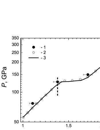
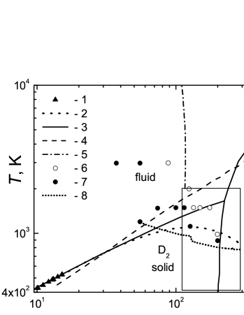
Figure 1: Deuterium quasi-isentropic compression. Experiment: 1 —[28]. This work: 2 — Widom’s test particle method, 3 — Zel’dovich’s method. Vertical line shows the density at which a sharp electircal conductivity rise is observed experimentally [27, 32].

Figure 2: Deuterium phase diagram. Melting curve: 1 — experiment [33]; 2 — extrapolation of experiment [33]. Theoretical phase diagram: 3 —[34]; 4 —[35]. Boundary of the possible phase transition: 5 —[29]. Atomic fluid: 6 —[30, 31]. Molecular liquid: 7 —[30, 31]. This work: 8 — isentrope; the black rectangle shows the region of slow convergence to the equilibrium state.

3.2 Quantum momentum-momentum correlation functions

We now compute the dynamic conductivity of a strongly coupled hydrogen plasma. The results obtained were practically insensitive to the variation of the whole number of particles in the Monte Carlo cell from 30 up to 60 and also to the number $n$ of high temperature density matrices in the path integral representation of the initial state which ranged from $n=20$ to 40. Estimates of the average statistical error gave a value of the order 5–7%. According to the Kubo formula [7] our calculations include two stages: (i) generation of the initial conditions (configuration of protons and electrons) in the canonical ensemble with the probability being proportional to the quantum density matrix and (ii), generation of the dynamic trajectories in phase space, starting from these initial configurations.

First we discuss the momentum-momentum autocorrelation functions (MMCF) which are shown in Fig. 3 for various temperatures and densities. The plasma density is characterized by the Brueckner parameter $r_{s}$ defined as the ratio of the mean interparticle distance $d=(\frac{3}{4\pi(n_{e}+n_{p})})^{1/3}$ to the Bohr radius $a_{B}$, where $n_{e}$ and $n_{p}$ are the electron and proton densities. The monotonic decay of the MMCF at low density transforms into aperiodic oscillations at high densities. The tails of the MMCF clearly show collective plasma oscillations. The damping time of the initial decay of the MMCF is strongly affected by variations of density and temperature. At constant density the decay time is at least two times smaller for $T=200\,000$ K compared to $T=50\,000$ K. As it follows from Fig. 3 the damping time is also sensitive to the density. The damping time of the MMCF increases when the density increases. The physical reason is the tendency towards ordering of the charges.

Figure 3: Typical MMCF in canonical ensemble for different densities ($r_{s}$) and three temperatures: $T=200\,000$ K (left), $T=100\,000$ K (central) and $T=50\,000$ K (right). Time is presented in atomic units.

3.3 Electrical conductivity

Figure 4 presents the real part of the diagonal elements of the electrical conductivity tensor versus frequency computed from the real part of the Fourier transform of the MMCF which characterizes the Ohmic absorption of electromagnetic energy. Collective plasma oscillations give the main contribution in the region of $\omega/\omega_{p}\sim 1$, where $\omega_{p}^{2}=4\pi n_{e}e^{2}/m_{e}$ is the plasma frequency. Reliable numerical data in this region require very long dynamic trajectories. Their initial parts are presented in Fig. 3. The high frequency tails of the dynamic conductivities coincide with analytical Drude-like expressions for fully ionized hydrogen plasma obtained in [4, 36]. For low frequency analytical estimations are going to infinity and this is the reason of discrepancy between numerical results and analytical estimations. With increasing plasma density non-monotonic behavior of the dynamic conductivity in the region of several plasma frequencies is observed. These oscillations can be an indication of the transparency window (low absorption coefficient) of the strongly coupled hydrogen plasma.

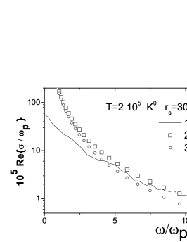
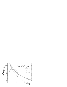
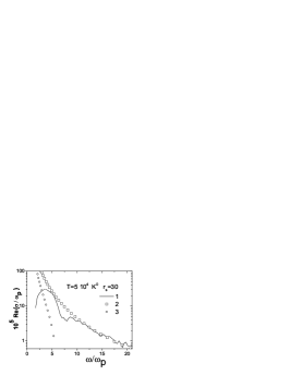
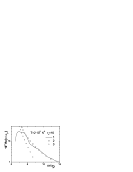
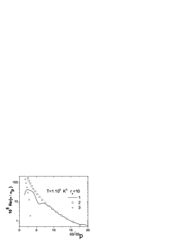
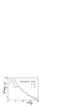
Figure 4: Real part of the Fourier transform of the MMCF (line 1) for densities related to three temperatures: $T=200\,000$ K (left column), $T=100\,000$ K (central column) and $T=50\,000$ K (right column) and to $r_{s}=30$ (top row) and $r_{s}=10$ (bottom row). Points $2$ and $3$ present analytical results obtained according to [37, 4] respectively. Frequency and scaled dynamic conductivity is given in units of plasma frequency.

The agreement with Drude-like formulas for weakly coupled plasma is due to the fact that the main contribution to the high frequency region comes from the fast trajectories with high (virtual) energy. This means that interaction of electrons with each other and protons only weakly disturbs the behavior of the high-frequency tails of dynamic conductivity in comparison with ideal plasma. Now let us consider the dynamic conductivity at very low plasma density, namely when the Brueckner parameter $r_{s}$ is equal to $43.2$. Fig. 5 presents MMCF and dynamic conductivity in a wide region of temperatures from $T=50\,000$ K up to $T=10\,000$ K. At temperatures lower than $T=50\,000$ K the plasma consists mainly of atoms. As a consequence the initial fast decay of the MMCF is modulated by the high frequency oscillations related to the motion of electrons inside the atoms. So the high frequency tail of the dynamic conductivity has a new maximum associated with the condition $Ry=\hbar\omega$. As it follows from Fig. 5 the position of this peak strongly depends on temperature and is shifted to lower frequency when temperature decreases. The physical reason is the growth of the energy levels population of hydrogen atoms with the increase of temperature. Analytical estimations for fully ionized plasma which are also presented in Fig. 5 give essentially larger values of dynamic conductivity.

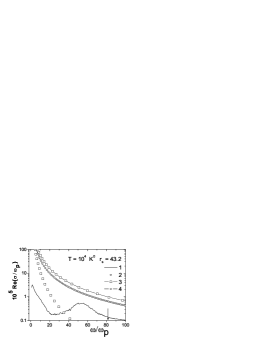
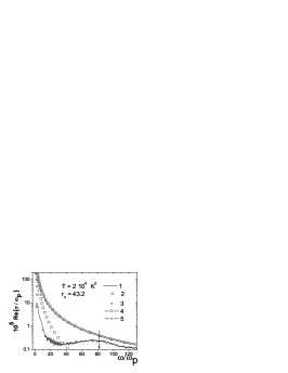
Figure 5: Typical MMCF in canonical ensemble for $r_{s}=43.2$ and four temperatures: $T=50\,000$ K, $T=20\,000$ K, $T=15\,000$ K and $T=10\,000$ K, time is presented in atomic units (left figure). Real part of the Fourier transform of MMCF (line 1) for density related to $r_{s}=43.2$ and temperatures $T=10\,000$ K (central figure) and $T=20\,000$ K (right figure). Data points 2–5 present analytical results obtained according to [37, 4, 36, 38] respectively. Arrow relates to the condition $Ry=\hbar\omega$.

4 Conclusion

We have used three approaches for the investigation of thermodynamic properties and electrical conductivity of dense hydrogen and deuterium plasma. Using two different methods of isentrope reconstruction from simulation results we obtained very good agreement with experimental data on quasi-isentropic compression of deuterium. We also applied the quantum dynamics approach to hydrogen plasma in a wide region of density and temperature. Calculating the MMCF we determined the dynamic electrical conductivity and compared the results with available theories. Our results show a strong dependence on the plasma coupling parameter. For low density and high temperature the numerical results agree well with the Drude approximation, while at higher values of the coupling parameter we observe a strong deviation of the frequency dependent conductivity and permittivity from low density and high temperature approximations.

References

References

- [1] Bezkrovniy V et al., Phys. Rev. E 70, 057401 (2004)
- [2] Johnson K J, Panagiotopoulos A Z and Gubbins K E 1994 Mol. Phys. 81 717
- [3] Zamalin V M, Norman G E and Filinov V S 1977 The Monte-Carlo Method in Statistical Thermodynamics (Moscow: Nauka)
- [4] Silin V P 1964 ZheTF 47 2254
- [5] Juranek H and Redmer R 2000 J. Chem. Phys. 112(8) 3780–3786
- [6] Liu L X and Su W L 2002 Int. J. Quant. Chem. 87 1–11
- [7] Zubarev D N 1974 Nonequilibrium Statistical Thermodynamics (New York: Plenum Press)
- [8] Filinov V S 1996 J. Mol. Phys. 88 1517–1529
- [9] Filinov V S, Lozovik Y, Filinov A, Zakharov E and Oparin A 1998 Physica Scripta 58 297–304
- [10] Kelbg G 1963 Ann. Physik 12 219
- [11] V. Filinov et al., Phys. Rev. B 65, 165124 (2002)
- [12] Zelener B V, Norman G E and Filinov V 1981 Perturbation theory and Pseudopotential in Statistical Thermodynamics (Moscow: Nauka)
- [13] Filinov V S 1975 High Temp. 13 1065
- [14] Zelener B V, Norman G E and Filinov V S 1975 High Temp. 13 650
- [15] Filinov V S, Bonitz M, Ebeling W and Fortov V E 2001 Plasma Phys. Cont. Fusion 43 743
- [16] Filinov V S, Bonitz M and Fortov V E 2000 JETP Letters 72 245
- [17] Filinov V S, Fortov V E, Bonitz M and Kremp D 2000 Phys. Lett. A 274 228
- [18] Filinov V S, Fortov V E, Bonitz M and Levashov P R 2001 JETP Letters 74(7) 384
- [19] Filinov A V, Bonitz M and Lozovik Y E 2001 Phys. Rev. Lett. 86 3851 and phys. stat. sol. (b) 221, 231 (2000)
- [20] Ciccotti G, Pierleoni C, Capuani F and V F 1999 Comp. Phys. Commun. 121–122 452–459
- [21] Lozovik Y and Filinov A 1999 Sov. Phys. JETP 88 1026
- [22] Widom B 1963 J. Chem. Phys. 39 2808
- [23] Arrieta E, Jedrzejek C and Marsh K N 1991 J. Chem. Phys. 95 6838
- [24] Zel’dovich Y B 1957 JETP 32 1577
- [25] Fortov V E and Krasnikov Y G 1970 JETP 59 1645
- [26] Levashov P R, Filinov V S, Botan A, Bonitz M and Fortov V E 2008 J. Phys.: Conf. Ser. 121 012012
- [27] Weir S T, Mitchell A C and Nellis W J 1996 Phys. Rev. Lett. 76 1860–1863
- [28] Fortov V E, et al., 2007 Phys. Rev. Lett. 99 185001
- [29] Beule D, et al., 1999 Phys. Rev. B 59 14177
- [30] Bonev S, Militzer B and Galli G 2004 Phys. Rev. B 69 014101
- [31] Scandolo S 2003 Proc. Nat. Ac. Sci. 100 3051
- [32] Ternovoi V Y, Filimonov A S, Fortov V E, Kvitov S V, Nikolaev D N and Pyalling A A 1999 Physica B 265 6–11
- [33] Datchi F, Loubeyre P and LeToullec R 2000 Phys. Rev. B 61 6535
- [34] Kerley G 1983 Molecular-Based Study of Fluids (Washington: American Chemical Society)
- [35] Fortov V E, Al’tshuler L V, Trunin R and Funtikov A I 2004 Shock Waves and Extreme States of Matter (New York: Springer-Verlag)
- [36] Mihajlov A A, Djurić Z, Adamyan V M and Sakan N M 2001 J. Phys. D: Appl. Phys. 34 3139
- [37] Bornath T, Schlanges M, Hilse P, Kremp D and Bonitz M 2000 Laser and Part. Beams 18 535
- [38] Adamyan V M, Grubor D, Mihajlov A A, Sakan N M, Srecovic V A and Tkachenko I 2006 J. Phys. A: Math. Gen. 39 4401