Asteroseismic age and radius of Kepler stars

Abstract

The Kepler mission’s primary goal is the detection and characterization of Earth-like planets by observing continuously a region of sky for a nominal period of three-and-a-half years. Over 100,000 stars will be monitored, with a small subset of these having a cadence of 1 minute, making asteroseismic studies for many stars possible. The subset of targets will consist of mainly solar-type and planet-hosting stars, and these will be observed for a minimum period of 1 month and a maximum depending on the scientific yield of the individual target. Many oscillation frequencies will be detected in these data, and these will be used to constrain the star’s fundamental parameters. I investigate the effect that an increase in a) the length of observation and b) the signal quality, has on the final determination of some stellar global parameters, such as the radius and the age.

Instituto de Astrofísica de Canarias, C/ Vía Lactea s/n, La Laguna 38205, Tenerife, Spain

High Altitude Observatory, 30801 Center Green Dr., Boulder, CO, 80301

1. Method

1.1. Precision of oscillation frequencies

The Kepler mission (Borucki et al. 1997, 2004) will yield high-cadence photometric time series for many hundreds to a few thousands of oscillating solar-type stars. By using any method to extract periodic signals in these light curves, for example an FFT or a least-squares fit to sinusoids, the pulsation frequencies or oscillation modes $\nu$ will be detectable. The number of frequencies detected for each star will depend primarily on the intrinsic brightness of the star, its distance and the characteristics of its oscillation modes. Consequently, the errors associated with each of the detected frequencies also depends on these characteristics. For data analysis purposes, however, we can quantify the error on each frequency $\epsilon_{\nu}$ as a function of signal-to-noise ratio (SNR) in the power spectrum, the duration of observation $T$ and the natural linewidth of the frequency $\Gamma$ (related to the damping rate of the oscillations). Libbrecht (1991) gives a formula for the estimation of these errors:

$$\epsilon_{\nu}^{2}=f(\beta)\frac{\Gamma}{4\pi T}$$ (1)

where $\beta$ is the inverse of the SNR and varies usually between 0.1 - 1.0.

1.2. Determining the constraints on global parameters

In order to determine the global parameters (and subsequently the internal structure) of a star, one needs to compare a set of model observables B to a set of observations O. We use a stellar structure and evolution code ASTEC (Christensen-Dalsgaard 1982, 2007a), coupled to an adiabatic oscillation code ADIPLS (Christensen-Dalsgaard 2007b). This model takes a set of input parameters P and generates a stellar model based on P. The expected observables B can be consequently calculated ($L_{\star}$, magnitudes, mean density …). One form of determining the stellar global parameters (these are the P) is to incorporate some algorithm that minimizes the discrepancies between the model observables and the observations, and then use a value (such as $\chi^{2}$) to quantify the fit to the data:

$$\chi^{2}=\sum_{i=1}^{M}\frac{(O_{i}-B_{i})^{2}}{\epsilon_{i}^{2}},$$ (2)

for each $i=1,...,M$ observation and $\epsilon_{i}$ represents the errors on each of the $O_{i}$.

Once we find a robust fit to the data, we can use the following formula to calculate the uncertainties in each of the model parameters:

$$\sigma_{j}^{2}=\sum_{k=1}^{N}\frac{V_{jk}^{2}}{W_{kk}^{2}}$$ (3)

for each $j=1,...,N$ model parameter. Here, $V_{k}$ and $W_{k}$ are the $k^{\rm th}$ components of the singular value decomposition of the matrix D, whose elements $D_{ij}$ are given by $\frac{\partial B_{i}}{\partial P_{j}}/\epsilon_{i}$ (Press et al. 1992; Brown et al. 1994; Creevey et al. 2007).

Here we can see that the uncertainties in the parameters such as mass, radius and age come from the sensitivity of each of the observables with respect to each of the parameters (from models), and the associated error on each of these measurements. These quantities can change by

• including more measurements, such as classical observations ($T_{\rm eff}$, $\log g$, $\log Z/X$) or more oscillation frequencies

• studying a star at various evolutionary stages, because the measurement sensitivities to each of the parameters changes as the stellar structure changes

• varying the expected errors on the measurements $\epsilon$.

In the first subsection we discussed the frequency errors and their dependencies on the photometric time series. Here we translate these into uncertainties in the global parameters of radius and age as a function of quality of data and duration of observations.

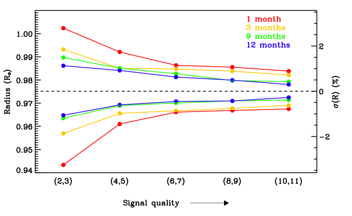
Figure 1.: Expected uncertainties in the radius of a 1 M_⊙ star as a function of signal quality. Each of the color curves represents the results for a specific duration of uninterrupted observations. The axis on the right shows the relative uncertainties.

2. Results

We show in Figures 1 and 2 the expected uncertainties in the radius and the age, respectively, of a 1 M_⊙ star as a function of signal quality. We have quantified signal quality as (SNR, NF) where the ’signal’ in SNR refers to the amplitude of the highest peak in the spectrum, and the ’noise’ refers to the noise level around this peak. NF is the number of detected frequencies for each oscillation mode $l=0$ and 1 i.e. NF = 3 means 3 $l$ = 0 modes and 3 $l$ = 1 modes.

If a star has a SNR of 10, then it is most likely that the number of detected frequencies (NF) in the power spectrum is higher than a star whose SNR = 2. For this reason we may assume that both the SNR and NF increase together. These are the numbers on the x-axis in each graph: e.g. (SNR, NF) = (2, 3), (4, 5) etc.

Both figures also show the uncertainties in the radius and the age assuming various lengths of observation. The various colour curves represent data of a specific time span of high-cadence 100% duty cycle observations: red, yellow, green and blue indicate respectively, 1 month, 3 months, 9 months and 12 months of observational data to extract the oscillation frequencies.

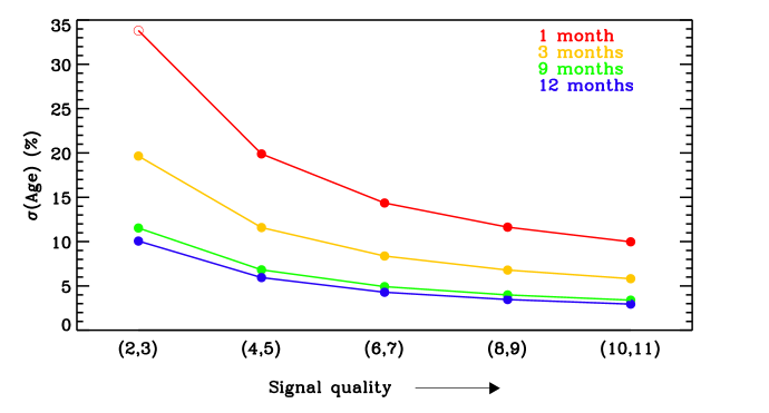
Figure 2.: Expected uncertainties in the age of a 1 M_⊙ star. See Figure 1 for details.

3. Conclusions

• The stellar radius can be determined to within 2-3% for a 1 M_⊙ star for all combinations of signal quality and observation length studied.

• Observing a star that has at least 5 detected frequencies for $l$=0 and $l$=1 modes yields $\sigma(\tau)<$20%, where $\tau$ is the age, and requiring that the length of observation is at least 3 months, improves this to better than 12%.

• The most significant improvements in $\sigma(R)$ and $\sigma(\tau)$ come from extending a data set from 1 month to 3 months. If the data set spans 9 months, then extending it will result in very little improvement in these quantities.

• A star observed for 1 month requires a minumum (SNR, NF) = (6, 7) to constrain adequately the radius and the age of a 1 M_⊙; 3 months requires a minimum (SNR, NF) = (4, 5); 9 months requires a minimum (SNR, NF) = (2, 3).

Acknowledgments.

OLC wishes to acknowledge Thierry Appourchaux, William J. Chaplin, Guenter Houdek, Sebastian Jiménez-Reyes, Hans Kjeldsen, Travis Metcalfe and David Salabert for discussions on various aspects of this work. OLC also wishes to acknowledge the ISSI for financial support for the “AsteroFLAG” meeting, where this idea was elaborated upon, and travel support was provided by the AAS International Travel Grant. This research was in part supported by the European Helio- and Asteroseismology Network (HELAS), a major international collaboration funded by the European Commission’s Sixth Framework Programme.

References

- Borucki et al. (1997) Borucki et al., 1997, ASPCS, 119, 153
- Borucki et al. (2004) Borucki et al., 2004, ESA SP-538, 177
- Brown et al. (1994) Brown et al., 1994, ApJ, 427, 1013
- Christensen-Dalsgaard (1982) Christensen-Dalsgaard, J. 1982, MNRAS, 199, 735
- Christensen-Dalsgaard (2007a) Christensen-Dalsgaard, J. 2007, arXiv:0710.3114
- Christensen-Dalsgaard (2007b) Christensen-Dalsgaard, J. 2007, arXiv:0710.3106
- Creevey et al. (2007) Creevey et al., 2007, ApJ, 659, 616
- Libbrecht (1991) Libbrecht, K.G. 1991, ApJ, 387, 712
- Press et al. (1992) Press et al. 1992 Numerical Recipes, Cambridge University Press