One of the main motivations for low energy supersymmetric theories is their ability to address the hierarchy and naturalness problems in the Higgs sector of the Standard Model. In these theories, at least two doublets of scalar fields are required to break the electroweak symmetry and to generate the masses of the elementary particles, resulting in a rather rich Higgs spectrum. The search for the Higgs bosons of Supersymmetry and the determination of their basic properties is one of the major goals of high–energy colliders and, in particular, the LHC which will soon start operation. We review the salient features of the Higgs sector of the Minimal Supersymmetric Standard Model and of some of its extensions and summarize the prospects for probing them at the LHC and at the future ILC.

1 Introduction

It was known relatively soon after the introduction of the Standard Model (SM) of the electroweak interactions [1], which makes use of one Higgs doublet of complex scalar fields to spontaneously break the ${\rm SU(2)_{L}\times U(1)_{Y}}$ symmetry to generate in a gauge invariant way the masses of the $W^{\pm},Z$ gauge bosons and the fermions [2], that the model suffers from a severe flaw: the so–called naturalness or fine–tuning problem [3]. Indeed, when attempting to calculate the quantum corrections to the squared mass of the single Higgs boson of the theory, one encounters divergences that are quadratic in the cut–off scale $\Lambda$ beyond which the theory ceases to be valid and new physics should appear. If one chooses the cut–off $\Lambda$ to be the Grand Unification (GUT) scale $M_{\rm GUT}\simeq 2\cdot 10^{16}$ GeV or the Planck scale $M_{\rm Pl}\sim 10^{18}$ GeV, the mass of the Higgs particle, which is expected for consistency reasons to lie in the range of the electroweak symmetry breaking scale $v\sim 250$ GeV, will prefer to be close to the very high scale unless an unnatural fine adjustment of parameters is performed. A related issue, called the hierarchy problem, is why these two scales are so widely different, $\Lambda\gg v$, a question that has no satisfactory answer in the SM.

Supersymmetry (SUSY), introduced in the early seventies by Julius Wess and Bruno Zumino [4, 5] among others [6] mainly for aesthetical reasons, is presently widely considered as the most attractive extension of the SM. The main reason is that it solves, at least technically, the hierarchy and naturalness problems [7]. Indeed, this new symmetry prevents the Higgs boson mass from acquiring large radiative corrections: the quadratic divergent loop contributions of the SM particles are exactly canceled by the corresponding loop contributions of their supersymmetric partners which differ in spin by $\frac{1}{2}$. This cancellation thus stabilizes the huge hierarchy between the GUT and the electroweak scales and no extreme fine-tuning is required. Later on, two other main motivations for introducing low energy supersymmetry in particle physics were recognized: the satisfactory unification of the gauge couplings of the electromagnetic, weak and strong interactions at the GUT scale [8] and the presence of a particle that is massive, electrically neutral, weakly interacting, absolutely stable, which is the ideal candidate for the dark matter in the universe [9].

The most intensively studied low energy supersymmetric extension of the SM is the most economical one, the so–called MSSM [10, 11, 12]. In this minimal model, one assumes the SM gauge group (and associates a spin–$\frac{1}{2}$ gaugino to each gauge boson of the model), the minimal particle content (in particular, three generations of fermions without right–handed neutrinos and their spin–zero partners, the sfermions) and the conservation of a discrete symmetry called R–parity which makes the lightest SUSY particle absolutely stable. In order to explicitly break SUSY, a collection of soft terms (i.e. which do not reintroduce quadratic divergences) is added to the Lagrangian [13, 14]: mass terms for the spin $\frac{1}{2}$ gauginos and the spin–0 sfermions, mass and bilinear terms for the Higgs bosons and trilinear couplings between sfermions and Higgs bosons. Although incomplete (e.g. it does not have right–handed (s)neutrinos and has a problem with the $\mu$ parameter), it serves as a benchmark scenario for the possible phenomenology of SUSY theories.

The MSSM requires the existence of two isodoublets of complex scalar fields of opposite hypercharge to cancel chiral anomalies and to give masses separately to isospin up–type and down–type fermions [7]. Three of the original eight degrees of freedom of the scalar fields are absorbed by the $W^{\pm}$ and $Z$ bosons to build their longitudinal polarizations and to acquire masses. The remaining degrees of freedom will correspond to five scalar Higgs bosons. In the absence of CP–violation, two CP–even neutral Higgs bosons $h$ and $H$, a pseudoscalar $A$ boson and a pair of charged scalar particles $H^{\pm}$ are thus introduced by this extension of the Higgs sector [15, 16, 17, 18, 19]. Besides the four masses, two additional parameters define the properties of these particles at tree–level: a mixing angle $\alpha$ in the neutral CP–even sector and the ratio of the two vacuum expectation values $\tan\beta$, which, from GUT restrictions, is assumed in the range $1\raisebox{-3.69899pt}{~{}\shortstack{$<$ \\ [-0.07cm] $\sim$}}~{}\tan\beta\raisebox{-3.69899pt}{~{}\shortstack{$<$ \\ [-0.07cm] $\sim$}}~{}m_{t}/m_{b}$ with the lower and upper ranges being favored if the Yukawa couplings are to be unified at the GUT scale [20]. Supersymmetry leads to several relations among these parameters and only two of them, taken in general to be the pseudoscalar Higgs mass $M_{A}$ and $\tan\beta$, are in fact independent. These relations impose a strong hierarchical structure on the mass spectrum, $M_{h}<M_{Z},M_{h}<M_{A}<M_{H}$ and $M_{W}<M_{H^{\pm}}$, which is, however, broken by radiative corrections [21, 22, 23, 24, 25]. These radiative corrections turn out to be very large and, for instance, they shift the upper bound on the mass of the lighter $h$ boson from the tree–level value $M_{Z}$ up to $M_{h}\sim 140$ GeV [23, 24]. Thus, in the MSSM, one Higgs particle is expected to be relatively light, while the masses of the heavier neutral and charged Higgs particles are expected to be in the range of the electroweak scale.

The Higgs sector in SUSY models may be more complicated if some basic assumptions of the CP–conserving MSSM, such as the absence of new sources of CP violation, the presence of only two Higgs doublets, or R–parity conservation, are relaxed. For instance, if CP–violation is present in the SUSY sector (which is required if baryogenesis is to be explained at the weak scale), the new phases will enter the MSSM Higgs sector through the large radiative corrections and alter the Higgs masses and couplings; in particular, the three neutral Higgs states will not have definite CP quantum numbers and will mix with each other to produce the physical states [26, 27]. Another interesting extension is the next–to–minimal supersymmetric SM, the NMSSM, which consists of simply introducing a complex iso-scalar field which naturally generates a weak scale value for the supersymmetric Higgs–higgsino parameter $\mu$ (thus solving the so–called $\mu$ problem) [28, 29]. The model includes an additional CP–even and CP–odd Higgs particles compared to the MSSM [29, 30].

A large variety of theories, string theories, Grand Unified theories, left–right symmetric models, etc., suggest an additional gauge symmetry which may be broken only at the TeV scale, leading to an extended particle spectrum and, in particular, to additional Higgs fields beyond the minimal set of the MSSM [31, 32, 33]. These extensions also predict extra matter fields and would lead to a very interesting phenomenology and new collider signatures in the Higgs sector. In a general SUSY model with an arbitrary number of singlet and doublet scalar fields (as well as a matter content which allows for the unification of the gauge couplings), a linear combination of Higgs fields has to generate the $W^{\pm}/Z$ masses and, from the requirement that all couplings stay perturbative up to $M_{\rm GUT}$, a Higgs particle should have significant couplings to gauge bosons and a mass below 200 GeV [34]. This sets an upper bound on the lighter Higgs particle mass in SUSY theories.

The phenomenology of the SUSY Higgs sector is thus much richer than the one of the SM with its unique Higgs boson. The study of the properties of the Higgs bosons and of those of the supersymmetric particles is one of the most active fields of elementary particle physics. The search for these new particles and, if discovered, the determination of their fundamental properties, is one of the major goals of high–energy colliders. In this context, the probing of the Higgs sector has a double importance since, at the same time, it provides the clue of the electroweak symmetry breaking mechanism and it sheds light on the SUSY–breaking mechanism. Moreover, while SUSY particles are allowed to be relatively heavy unless one invokes fine–tuning arguments, the existence of a light Higgs boson is a generic prediction of low energy SUSY. This particle should therefore manifest itself at the next round of high–energy experiments, in particular at the LHC [35, 36, 37, 38, 39, 40], which will start operation rather soon, and at the future ILC [40, 41, 42, 43]. We are thus in a situation where either SUSY with its extended Higgs sector is discovered soon or, in the absence of a light Higgs boson, the whole SUSY edifice, at least in the way it is presently viewed, collapses.

This review summarizes the salient features of the Higgs sector of SUSY theories. In the two next sections, we present the Higgs spectrum of the MSSM and some of its extensions, and summarize the decays of and into the Higgs bosons. In sections 4 and 5, we discuss the production, the detection and the study of the properties of the Higgs particles at the LHC and at the future ILC. A very brief conclusion is given in Section 6. A short Appendix collects some basic formulae.

2 The Higgs spectrum in SUSY models

2.1 The Higgs potential of the MSSM

In the MSSM, two doublets of complex scalar fields of opposite hypercharge are required

$$H_{1}=\left(\begin{array}[]{cc}H^{0}_{1}\\ H^{-}_{1}\end{array}\right)\ {\rm with}\ Y_{H_{1}}=-1\ \ ,\ \ H_{2}=\left(\begin{array}[]{cc}H^{+}_{2}\\ H^{0}_{2}\end{array}\right)\ {\rm with}\ Y_{H_{2}}=+1\ ,$$ (5)

to break spontaneously the electroweak symmetry. There are several reasons for this requirement.

The first reason is that in the SM, one generates the masses of the fermions of a given isospin by using the same scalar field $\Phi$ that also generates the $W$ and $Z$ boson masses, the isodoublet $\tilde{\Phi}=i\tau_{2}\Phi^{*}$ with opposite hypercharge generating the masses of the opposite isospin–type fermions. However, in a SUSY theory, the Superpotential should involve only the superfields and not their conjugate fields. Therefore, we must introduce a second doublet with the same hypercharge as the conjugate $\tilde{\Phi}$ field to generate the masses of both isospin–type fermions [7, 10].

A second reason is that in the SM, chiral anomalies which spoil the renormalizability of the theory, disappear because the sum of the hypercharges or charges of all the 15 chiral fermions of one generation is zero, ${\rm Tr}(Y_{f})={\rm Tr}(Q_{f})=0$. In the SUSY case, if we use only one doublet of Higgs fields as in the SM, we will have one additional charged spin $\frac{1}{2}$ particle, the higgsino corresponding to the SUSY partner of the charged component of the scalar field, which will spoil this cancellation. With two doublets of Higgs fields with opposite hypercharge, the cancellation of chiral anomalies still takes place [44] and the renormalizability of the theory is preserved.

Finally, a higher number of Higgs doublets would spoil the unification of the electromagnetic, weak and strong coupling constants at the GUT energy scale if no additional matter particles are added to the spectrum; see for instance Ref.  [34].

In the MSSM, the terms contributing to the scalar Higgs potential $V_{H}$ come from various sources; see the Appendix. The potential can be written as [15, 16, 12]:

$$V_{H} = (|\mu|^{2}+m_{H_{1}}^{2})|H_{1}|^{2}+(|\mu|^{2}+m_{H_{2}}^{2})|H_{2}|^{2}-\mu B\epsilon_{ij}(H_{1}^{i}H_{2}^{j}+{\rm h.c.})$$ (6)

$$+{g_{2}^{2}+g_{1}^{2}\over 8}(|H_{1}|^{2}-|H_{2}|^{2})^{2}+{1\over 2}g_{2}^{2}|H_{1}^{\dagger}H_{2}|^{2}$$

where $m_{H_{1}},m_{H_{2}}$ are the soft–SUSY breaking terms for the Higgs boson masses and $B\mu$ is the one of the bilinear term $\mu H_{1}H_{2}$ of the SUSY Lagrangian; $g_{2}$ and $g_{1}$ are the ${\rm SU(2)_{L}}$ and ${\rm U(1)_{Y}}$ couplings and $\epsilon_{12}=1=-\epsilon_{21}$. Defining the mass squared terms

$$\overline{m}_{1}^{2}=|\mu|^{2}+m_{H_{1}}^{2}\,,\,\ \overline{m}_{2}^{2}=|\mu|^{2}+m_{H_{2}}^{2}\,,\,\ \overline{m}_{3}^{2}=B\mu$$ (7)

one obtains, using the decomposition of the $H_{1,2}$ fields into neutral and charged components eq. (5)

$$V_{H} = \overline{m}_{1}^{2}(|H_{1}^{0}|^{2}+|H^{-}_{1}|^{2})+\overline{m}_{2}^{2}(|H_{2}^{0}|^{2}+|H_{2}^{+}|^{2})-\overline{m}_{3}^{2}(H_{1}^{-}H_{2}^{+}-H_{1}^{0}H_{2}^{0}+{\rm h.c.})$$ (8)

$$+{g_{2}^{2}+g_{1}^{2}\over 8}(|H_{1}^{0}|^{2}+|H_{1}^{-}|^{2}-|H_{2}^{0}|^{2}-|H_{2}^{+}|^{2})^{2}+{g_{2}^{2}\over 2}|H_{1}^{-*}H_{1}^{0}+H_{2}^{0*}H_{2}^{+}|^{2}$$

One can then require that the minimum of the potential $V_{H}$ breaks the ${\rm SU(2)_{L}\times U(1)_{Y}}$ group while preserving the electromagnetic symmetry U(1)_Q. At the minimum of the potential, one can always choose the vacuum expectation value of the field $H_{1}^{-}$ to be zero, $\langle H^{-}_{1}\rangle$=0, because of SU(2) symmetry. At $\partial V/\partial H^{-}_{1}$=0, one obtains then automatically $\langle H^{+}_{2}\rangle$=0. There is therefore no breaking in the charged directions and the QED symmetry is preserved. Some interesting and important remarks on the potential $V_{H}$ can be made [15, 16, 12]:

$\bullet$ The quartic Higgs couplings are fixed in terms of the ${\rm SU(2)_{L}\times U(1)_{Y}}$ gauge couplings. Contrary to a general two–Higgs doublet model where the scalar potential has 6 free parameters and a phase, in the MSSM we have only three free parameters: $\overline{m}^{2}_{1},\overline{m}^{2}_{2}$ and $\overline{m}^{2}_{3}$.

$\bullet$ The two combinations $m_{H_{1},H_{2}}^{2}+|\mu|^{2}$ are real and, thus, only $B\mu$ can be complex. However, any phase in $B\mu$ can be absorbed into the phases of the fields $H_{1}$ and $H_{2}$. Thus, the scalar potential of the MSSM is CP conserving at the tree–level.

$\bullet$ To have electroweak symmetry breaking, one needs a combination of the $H_{1}^{0}$ and $H_{2}^{0}$ fields to have a negative squared mass term. This occurs if $\overline{m}_{3}^{2}>\overline{m}_{2}^{2}\overline{m}_{2}^{2}$. If not, $\langle H_{1}^{0}\rangle=\langle H_{2}^{0}\rangle$ will be a stable minimum of the potential and there is no electroweak symmetry breaking (EWSB).

$\bullet$ In the direction $|H_{1}^{0}|$=$|H_{2}^{0}|$, there is no quartic term. $V_{H}$ is bounded from below for large values of the field $H_{i}$ only if the condition $\overline{m}_{1}^{2}+\overline{m}_{2}^{2}>2|\overline{m}_{3}^{2}|$ is satisfied.

$\bullet$ To have explicit electroweak symmetry breaking and, thus, a negative squared term in the Lagrangian, the potential at the minimum should have a saddle point which implies $\overline{m}_{1}^{2}\overline{m}_{2}^{2}<\overline{m}_{3}^{4}$.

$\bullet$ The two above conditions on the masses $\overline{m}_{i}$ are not satisfied if $\overline{m}_{1}^{2}=\overline{m}_{2}^{2}$ and, thus, we must have non–vanishing soft SUSY–breaking scalar masses: $\overline{m}_{1}^{2}\neq\overline{m}_{2}^{2}$ meaning $m_{H_{1}}^{2}\neq m_{H_{2}}^{2}$.

Therefore, to break the electroweak symmetry, we need also to break SUSY. This provides a close connection between gauge symmetry breaking and SUSY–breaking. In constrained models such as the minimal supergravity model [14], the soft SUSY–breaking scalar Higgs masses are equal at high–energy, $m_{H_{1}}=m_{H_{2}}$ [and their squares positive], but the running to lower energies via the contributions of top/bottom quarks and their SUSY partners in the renormalization group evolution (RGE) makes that this degeneracy is lifted at the weak scale, thus satisfying the relation $m_{H_{1}}^{2}\neq m_{H_{2}}^{2}$ above. In the running one obtains $m_{H_{2}}^{2}<0$ or $m_{H_{2}}^{2}\ll m_{H_{1}}^{2}$ which thus triggers EWSB: this is the radiative breaking of the symmetry [45]. Thus, EWSB is more natural and elegant in the MSSM than in the SM since, in the latter case, one needs to make the ad hoc choice of a negative mass squared term for the scalar field in the Higgs potential while, in the MSSM, this comes simply from radiative corrections.

2.2 The masses of the MSSM Higgs bosons

Let us now determine the Higgs spectrum in the CP–conserving MSSM, following Refs. [15, 16, 12]. The neutral components of the two Higgs fields develop vacuum expectations values

$$\langle H_{1}^{0}\rangle=v_{1}/\sqrt{2}\ \ ,\ \ \langle H_{2}^{0}\rangle=v_{2}/\sqrt{2}$$ (9)

Minimizing the scalar potential at the electroweak minimum, $\partial V_{H}/\partial H_{1}^{0}=\partial V_{H}/\partial H_{2}^{0}=0$, using

$$(v_{1}^{2}+v_{2})^{2}=v^{2}=4M_{Z}^{2}/(g_{2}^{2}+g_{1}^{2})=(246~{}{\rm GeV})^{2}$$ (10)

with $v$ the SM vacuum expectation value, and defining the important parameter

$$\tan\beta=v_{2}/v_{1}=(v\sin\beta)/(v\cos\beta)$$ (11)

one obtains two minimization conditions that can be written in the following way:

$$2B\mu = (m_{H_{1}}^{2}-m_{H_{2}}^{2})\tan 2\beta+M_{Z}^{2}\sin 2\beta$$

$$\mu^{2}\cos\beta = (m_{H_{2}}^{2}\sin^{2}\beta-m_{H_{1}}^{2}\cos^{2}\beta)-M_{Z}^{2}\cos 2\beta/2$$ (12)

These relations show explicitly what we have already mentioned: if $m_{H_{1}}$ and $m_{H_{2}}$ are known (e.g. from RGEs once fixed at the scale $M_{\rm GUT}$) and $\tan\beta$ is fixed at the weak scale, $B$ and $\mu^{2}$ are fixed while the sign of $\mu$ stays undetermined. These relations are very important as the requirement of radiative EWSB leads to additional constraints and lowers the number of free parameters.

To obtain the Higgs physical fields and their masses, one has to develop the two doublet complex scalar fields $H_{1}$ and $H_{2}$ around the vacuum, into real and imaginary parts

$$H_{1}=(H_{1}^{0},H_{1}^{-})=\frac{1}{\sqrt{2}}\left(v_{1}+H_{1}^{0}+iP_{1}^{0},H_{1}^{-}\right)\ ,\ H_{2}=(H_{2}^{+},H_{2}^{0})=\frac{1}{\sqrt{2}}\left(H_{2}^{+},v_{2}+H_{2}^{0}+iP_{2}^{0}\right)$$ (13)

where the real parts correspond to the CP–even Higgses and the imaginary parts to the CP–odd Higgs and Goldstone bosons, and then diagonalize the mass matrices evaluated at the vacuum

$${\cal M}_{ij}^{2}=\frac{1}{2}\left.\frac{\partial^{2}V_{H}}{\partial H_{i}\partial H_{j}}\right|_{\langle H_{1}^{0}\rangle=v_{1}/\sqrt{2},\langle H_{2}^{0}\rangle=v_{2}/\sqrt{2},\langle H^{\pm}_{1,2}\rangle=0}$$ (14)

In the case of the CP–even Higgs bosons, one obtains the following mass matrix

$${\cal M}_{R}^{2}=\left[\begin{array}[]{cc}-\bar{m}_{3}^{2}\tan\beta+M_{Z}^{2}\cos^{2}\beta&\bar{m}_{3}^{2}-M_{Z}^{2}\sin\beta\cos\beta\\ \bar{m}_{3}^{2}-M_{Z}^{2}\sin\beta\cos\beta&-\bar{m}_{3}^{2}{\rm cot}\beta+M_{Z}^{2}\sin^{2}\beta\end{array}\right]$$ (17)

while for the neutral Goldstone and CP–odd Higgs bosons, one has the mass matrix

$${\cal M}_{I}^{2}=\left[\begin{array}[]{cc}-\bar{m}_{3}^{2}\tan\beta&\bar{m}_{3}^{2}\\ \bar{m}_{3}^{2}&-\bar{m}_{3}^{2}{\rm cot}\beta\end{array}\right]$$ (20)

In the latter case, since Det$({\cal M}_{I}^{2})=0$, one eigenvalue is zero and corresponds to the Goldstone boson mass, while the other corresponds to the pseudoscalar Higgs mass and is given by

$$M_{A}^{2}=-\bar{m}_{3}^{2}(\tan\beta+{\rm cot}\beta)=-2\bar{m}_{3}^{2}/\sin 2\beta$$ (21)

The mixing angle $\theta$ which gives the physical fields is in fact simply the angle $\beta$

$$\left(\begin{array}[]{c}G^{0}\\ A\end{array}\right) = {\cal R}_{\beta}\left(\begin{array}[]{c}P_{1}^{0}\\ P_{2}^{0}\end{array}\right)=\left(\begin{array}[]{cc}\cos\beta&\sin\beta\\ -\sin\beta&\cos\beta\end{array}\right)\ \left(\begin{array}[]{c}P_{1}^{0}\\ P_{2}^{0}\end{array}\right)$$ (30)

In the charged Higgs case, one can make the same exercise and obtain the charged fields, $(^{G^{\pm}}_{H^{\pm}})={\cal R}_{\beta}(^{H_{1}^{\pm}}_{H_{2}^{\pm}})$, with a massless charged Goldstone and a charged Higgs boson with a mass

$$M_{H^{\pm}}^{2}=M_{A}^{2}+M_{W}^{2}$$ (31)

Coming back to the CP–even Higgs case, one obtains then for the Higgs boson masses

$$M_{h,H}^{2}=\frac{1}{2}\left[M_{A}^{2}+M_{Z}^{2}\mp\sqrt{(M_{A}^{2}+M_{Z}^{2})^{2}-4M_{A}^{2}M_{Z}^{2}\cos^{2}2\beta}\right]$$ (32)

The physical Higgs bosons are obtained from the rotation of angle $\alpha$, $(^{H}_{h})={\cal R}_{\alpha}(^{H_{1}^{0}}_{H_{2}^{0}})$, where the mixing angle $\alpha$ is given in compact form by

$$\alpha=\frac{1}{2}{\rm arctan}\bigg{(}{\rm tan}2\beta\,\frac{M_{A}^{2}+M_{Z}^{2}}{M_{A}^{2}-M_{Z}^{2}}\bigg{)}\ ,\ \ -\frac{\pi}{2}\leq\alpha\leq 0$$ (33)

Thus, the supersymmetric structure of the theory has imposed very strong constraints on the Higgs spectrum. Out of the six parameters which describe the MSSM Higgs sector, $M_{h},M_{H},M_{A},M_{H^{\pm}},\beta$ and $\alpha$, only two parameters, which can be taken as $\tan\beta$ and $M_{A}$, are free parameters at the tree–level. In addition, a strong hierarchy is imposed on the mass spectrum and, besides the relations $M_{H}>{\rm max}(M_{A},M_{Z})$ and $M_{H\pm}>M_{W}$, we have the very important constraint on the lightest $h$ boson mass at the tree–level which is maximal for large $\tan\beta$ values for which $\cos 2\beta=1$,

$$M_{h} \leq {\rm min}(M_{A},M_{Z})\cdot|\cos 2\beta|\leq M_{Z}$$ (34)

2.3 The couplings of the MSSM Higgs bosons

The Higgs boson couplings to the gauge bosons [15, 16] are obtained from the kinetic terms of the fields $H_{1}$ and $H_{2}$ in the Lagrangian

$${\cal L}_{\rm kin.}=(D^{\mu}H_{1})^{\dagger}(D_{\mu}H_{1})+(D^{\mu}H_{2})^{\dagger}(D_{\mu}H_{2})$$ (35)

Expanding the covariant derivative $D_{\mu}=-ig_{2}\frac{1}{2}\tau_{a}W^{a}_{\mu}-ig_{1}\frac{Y}{2}B_{\mu}$ and performing the usual transformations on the gauge and scalar fields to obtain the physical fields, one can identify the trilinear couplings $V_{\mu}V_{\nu}H_{i}$ among one Higgs and two gauge bosons and $V_{\mu}H_{i}H_{j}$ among one gauge boson and two Higgs bosons, as well as the couplings between two gauge and two Higgs bosons $V_{\mu}V_{\nu}H_{i}H_{j}$. The Feynman rules for the important couplings of the neutral Higgs bosons are given below, where we have used the abbreviated couplings $g_{W}=g_{2}$ and $g_{Z}=g_{2}/c_{W}$ [$c_{W}^{2}=1-s_{W}^{2}\equiv\cos^{2}\theta_{W}$]:

$$Z_{\mu}Z_{\nu}h\ :\ ig_{Z}M_{Z}\sin(\beta-\alpha)g_{\mu\nu} Z_{\mu}Z_{\nu}H\ \ \ :\ ig_{Z}M_{Z}\cos(\beta-\alpha)g_{\mu\nu}$$ ,

$$W^{+}_{\mu}W^{+}_{\nu}h\ \ :\ ig_{W}M_{W}\sin(\beta-\alpha)g_{\mu\nu} W^{+}_{\mu}W^{-}_{\nu}H\ :\ ig_{W}M_{W}\cos(\beta-\alpha)g_{\mu\nu}$$ ,

$$Z_{\mu}hA:+{g_{Z}\over 2}\cos(\beta-\alpha)(p_{h}+p_{A})_{\mu} Z_{\mu}HA:-{g_{Z}\over 2}\sin(\beta-\alpha)(p_{H}+p_{A})_{\mu}$$ , (36)

with $p_{i}$ the (entering the vertex) momenta of the Higgs bosons. A few remarks are to be made:

$\bullet$ The couplings of the charged Higgs bosons follow closely those of the $A$ boson.

$\bullet$ Since the photon is massless, there are no Higgs–$\gamma\gamma$ and Higgs–$Z\gamma$ couplings at tree–level (there is no Higgs–gluon-gluon coupling as well as the Higgs is colorless) but the couplings can be generated at the loop level. CP–invariance also forbids $WWA,ZZA$ and $WZH^{\pm}$ couplings.

$\bullet$ For the $H_{i}H_{j}V$ couplings, CP–invariance implies that $H_{i}$ and $H_{j}$ must have opposite parity; there are no $Zhh,ZHh,ZHH,ZAA$ couplings and only the $ZhA$ and $ZHA$ couplings are allowed.

$\bullet$ There are many quartic couplings between two Higgs and two gauge bosons; they are proportional to $g_{\mu\nu}$ and involve two powers of the electroweak coupling which make them small.

$\bullet$ The couplings of the $h$ and $H$ bosons to $VV$ states are proportional to either $\sin(\beta-\alpha)$ or $\cos(\beta-\alpha)$; they are thus complementary and the sum of their squares is just the square of the SM Higgs boson coupling $g_{H_{\rm SM}VV}$. This complementarity will have very important consequences. For large $M_{A}$ values, one can expand the Higgs–VV couplings in powers of $M_{Z}/M_{A}$ to obtain

$$g_{HVV} \propto \cos(\beta-\alpha)\stackrel{{\scriptstyle\small M_{A}\gg M_{Z}}}{{\longrightarrow}}\ \ \frac{M_{Z}^{2}}{2M_{A}^{2}}\sin 4\beta\quad\ \stackrel{{\scriptstyle\small\tan\beta\gg 1}}{{\longrightarrow}}\quad-\frac{2M_{Z}^{2}}{M_{A}^{2}\tan\beta}\ \rightarrow 0$$

$$g_{hVV} \propto \sin(\beta-\alpha)\stackrel{{\scriptstyle\small M_{A}\gg M_{Z}}}{{\longrightarrow}}1-\frac{M_{Z}^{4}}{8M_{A}^{4}}\sin^{2}4\beta\stackrel{{\scriptstyle\small\tan\beta\gg 1}}{{\longrightarrow}}1-\frac{2M_{Z}^{4}}{M_{A}^{4}\tan^{2}\beta}\rightarrow 1$$ (37)

where we have also displayed the limits at large $\tan\beta$. One sees that for $M_{A}\gg M_{Z}$, $g_{HVV}$ vanishes while $g_{hVV}$ reaches unity, i.e. the SM value; this occurs more quickly if $\tan\beta$ is large.

As SUSY imposes that the doublet $H_{1}(H_{2})$ generates the masses and couplings of isospin $-\frac{1}{2}(+\frac{1}{2})$ fermions, Higgs mediated flavor changing neutral currents are automatically forbidden. The Higgs couplings to fermions come from the superpotential; using the left– and right–handed projection operators $P_{L/R}\!=\!\frac{1}{2}(1\!\mp\!\gamma_{5})$, the Yukawa Lagrangian with the first family notation is

$${\cal L}_{\rm Yuk} = -\lambda_{u}[\bar{u}P_{L}uH_{2}^{0}-\bar{u}P_{L}dH_{2}^{+}]-\lambda_{d}[\bar{d}P_{L}dH_{1}^{0}-\bar{d}P_{L}uH_{1}^{-}]+{\rm h.c.}$$ (38)

The fermion masses, generated when the Higgs fields acquire their vevs, are related to the Yukawa couplings by $\lambda_{u}\!=\!\sqrt{2}m_{u}/(v\sin\beta)$ and $\lambda_{d}\!=\!\sqrt{2}m_{d}/(v\cos\beta)$. Expressing the $H_{1}$ and $H_{2}$ fields in terms of the physical fields, one obtains the MSSM Higgs couplings to fermions [15, 16]

$$G_{huu}=i\frac{m_{u}}{v}\frac{\cos\alpha}{\sin\beta}\ ,\ \ G_{Huu}=i\frac{m_{u}}{v}\frac{\sin\alpha}{\sin\beta}\ ,\ \ G_{Auu}=\frac{m_{u}}{v}\cot\beta\,\gamma_{5}$$

$$G_{hdd}=-i\frac{m_{d}}{v}\frac{\sin\alpha}{\cos\beta}\ ,\ \ G_{Hdd}=i\frac{m_{d}}{v}\frac{\cos\alpha}{\cos\beta}\ ,\ \ G_{Add}=\frac{m_{d}}{v}\tan\beta\,\gamma_{5}$$

$$G_{H^{+}\bar{u}d}=-\frac{i}{\sqrt{2}v}V_{ud}^{*}[m_{d}\tan\beta(1+\gamma_{5})+m_{u}{\rm cot}\beta(1-\gamma_{5})]$$ (39)

One notices that the couplings of the $H^{\pm}$ bosons have the same $\tan\beta$ dependence as those of the pseudoscalar $A$ boson and that, for values $\tan\beta>1$, the $A$ and $H^{\pm}$ couplings to down–type (up–type) fermions are enhanced (suppressed). Thus, for large values of $\tan\beta$, the couplings of these Higgs bosons to $b$ quarks, $\propto m_{b}\tan\beta$, become very strong while those to the top quark, $\propto m_{t}/\tan\beta$, become rather weak. This is, in fact, also the case of the couplings of one of the CP–even Higgs boson $h$ or $H$ to fermions. depending on the magnitude of $\cos(\beta-\alpha)$. This can be viewed in the limit of very large $M_{A}$ values. In this case, the reduced Higgs couplings to fermions (normalized to the SM Higgs case) reach the limit:

$$M_{A}\gg M_{Z}:g_{huu}\to 1\ ,\ g_{hdd}\to 1\,\ g_{Huu}\to-\cot\beta\ ,\ g_{Hdd}\to\tan\beta$$ (40)

Thus, the couplings of the $h$ boson approach those of the SM Higgs boson, while the couplings of the $H$ boson reduce, up to a sign, to those of the pseudoscalar Higgs boson. Again, these limits are in general reached more quickly at large values of $\tan\beta$..

The trilinear and quadrilinear couplings between three or four Higgs fields can be obtained from the scalar potential $V_{H}$ by performing derivatives with respect to three or four Higgs fields. Two important trilinear couplings among neutral Higgs bosons, in units of $\lambda_{0}=-iM_{Z}^{2}/v$, are [15, 16]

$$\lambda_{hhh}=3\cos 2\alpha\sin(\beta+\alpha)\,,\ \lambda_{Hhh}=2\sin 2\alpha\sin(\beta+\alpha)-\cos 2\alpha\cos(\beta+\alpha)$$ (41)

The numerous quartic Higgs couplings involve two powers of the electroweak coupling and can be expressed in units of $\lambda_{0}/v=M_{Z}^{2}/v^{2}$; they are thus very small.

Finally, there are Higgs couplings to SUSY particles. A coupling which plays an important role is the $h$ coupling to top squarks which, in the case of the lightest one $\tilde{t}_{1}$, reads [17]

$$g_{h\tilde{t}_{1}\tilde{t}_{1}}\propto\cos 2\beta M_{Z}^{2}\left[\frac{1}{2}\cos^{2}\theta_{t}-\frac{2}{3}s^{2}_{W}\cos 2\theta_{t}\right]+m_{t}^{2}+\frac{1}{2}\sin 2\theta_{t}m_{t}X_{t}$$ (42)

and involves components which are proportional to $X_{t}=A_{t}-\mu\cot\beta$ where $A_{t}$ is the stop mixing parameter. For large values of the parameter $X_{t}$, which incidentally make the $\tilde{t}$ mixing angle almost maximal, $|\sin 2\theta_{t}|\simeq 1$ and lead to lighter $\tilde{t}_{1}$ states, the last components can strongly enhance the $g_{h\tilde{t}_{1}\tilde{t}_{1}}$ coupling and make it larger than the top quark coupling, $g_{htt}\propto m_{t}/M_{Z}$.

Another class of potentially important couplings of the Higgs bosons are the ones to the two charginos $\chi_{i}^{\pm}$ and four neutralinos $\chi_{i}^{0}$. With the notation $\Phi=h,H,A$, they are given by [17]

$$g_{\chi^{0}_{i}\chi^{+}_{j}H^{+}} \propto \sqrt{2}Z_{j4}V_{i1}+\left(Z_{j2}+\tan\theta_{W}Z_{j1}\right)V_{i2}$$

$$g_{\chi^{-}_{i}\chi^{+}_{j}\Phi}\propto e_{k}V_{j1}U_{i2}-d_{k}V_{j2}U_{i1} g_{\chi^{0}_{i}\chi^{0}_{j}\Phi}\propto\left(Z_{j2}-\tan\theta_{W}Z_{j1}\right)\left(e_{\Phi}Z_{i3}+d_{\Phi}Z_{i4}\right)$$ , (43)

where $Z$ and $U/V$ are the $4\times 4$ and $2\times 2$ matrices which diagonalize the neutralino and chargino matrices and the coefficients $e_{\Phi},d_{\Phi}$ are sines and cosines of the angles $\alpha$ and $\beta$. The Higgs couplings to the $\chi_{1}^{0}$ lightest SUSY particle (LSP), for which $Z_{11},Z_{12}$ are the gaugino components and $Z_{13},Z_{14}$ the higgsino components, vanish if the LSP is a pure gaugino or a pure higgsino. This statement can be generalized to all neutralino and chargino states and the Higgs bosons couple only to higgsino–gaugino mixtures or states. The couplings of the neutral Higgs bosons to neutralinos can also accidentally vanish for certain values of $\tan\beta$ and $\alpha$ which enter the coefficients $d_{\Phi},e_{\Phi}$.

2.4 Radiative corrections in the MSSM Higgs sector

It was realized in the early nineties that, as a result of the large Yukawa coupling of the top quark, the radiative corrections in the MSSM Higgs sector are very important [21]. The leading part of these corrections rise with the fourth power of the top quark mass and logarithmically with the stop mass. These corrections may push the lighter Higgs mass well above the tree–level bound, $M_{Z}$. In the subsequent years, an impressive theoretical effort has been devoted to the precise determination of the Higgs boson masses in the MSSM. A first step was to provide the full one–loop computation including the contributions of all SUSY particles [22] and a second the addition of the dominant two–loop corrections [23, 24] involving the strongest couplings of the theory, the QCD coupling and the Yukawa couplings of heavy third generation fermions. Other small higher–order corrections have also been calculated [25].

As seen previously, at the tree level, the Higgs sector of the MSSM can be described by two input parameters, which can be taken to be $M_{A}$ and $\tan\beta$. The CP–even Higgs mass matrix, given by eq. (17), receives radiative corrections at higher orders and it can be written as

$${\cal M}^{2}=\left[\begin{array}[]{cc}{\cal M}_{11}^{2}+\Delta{\cal M}_{11}^{2}&{\cal M}_{12}^{2}+\Delta{\cal M}_{12}^{2}\\ {\cal M}_{12}^{2}+\Delta{\cal M}_{12}^{2}&{\cal M}_{22}^{2}+\Delta{\cal M}_{22}^{2}\end{array}\right]$$ (46)

The leading one–loop radiative corrections $\Delta{\cal M}_{ij}^{2}$ to the mass matrix are controlled by the top Yukawa coupling $\lambda_{t}$ and one can obtain a very simple analytical expression in this case [21]

$$\Delta{\cal M}_{11}^{2} \sim \Delta{\cal M}_{12}^{2}\sim 0\ ,$$

$$\Delta{\cal M}_{22}^{2} \sim \epsilon=\frac{3\,\bar{m}_{t}^{4}}{2\pi^{2}v^{2}\sin^{2}\beta}\left[\log\frac{M_{S}^{2}}{\bar{m}_{t}^{2}}+\frac{X_{t}^{2}}{2\,M_{S}^{2}}\left(1-\frac{X_{t}^{2}}{6\,M_{S}^{2}}\right)\right]$$ (47)

where $M_{S}$ is the arithmetic average of the stop masses $M_{S}\!=\!\frac{1}{2}(m_{\tilde{t}_{1}}\!+\!m_{\tilde{t}_{2}})$, $X_{t}\!=\!A_{t}-\mu/\tan\beta$ where $A_{t}$ is the stop mixing parameter and $\bar{m}_{t}$ is the running ${\rm\overline{MS}}$ top quark mass to account for the leading two–loop QCD and electroweak corrections in a renormalization group (RG) improvement.

The corrections controlled by the bottom Yukawa coupling $\lambda_{b}$ are in general strongly suppressed by powers of the $b$–quark mass $m_{b}$. However, this suppression can be compensated by a large value of the sbottom mixing parameter $X_{b}=A_{b}-\mu\tan\beta$, providing a non–negligible correction to ${\cal M}^{2}$. Including these subleading contributions at one–loop, plus the leading logarithmic contributions at two–loops, provides a rather good approximation of the bulk of the radiative corrections. Nevertheless, one needs to include the full set of corrections mentioned previously to have precise predictions for the Higgs boson masses and couplings to which we turn now.

The radiatively corrected CP–even Higgs boson masses are obtained by diagonalizing the mass matrix eq. (46). In the approximation where only the leading corrections controlled by the top Yukawa coupling, eq. (47), are implemented, the masses are simply given by [21]

$$M_{h,H}^{2}=\frac{1}{2}(M_{A}^{2}+M_{Z}^{2}+\epsilon)\left[1\mp\sqrt{1-4\frac{M_{Z}^{2}M_{A}^{2}\cos^{2}2\beta+\epsilon(M_{A}^{2}\sin^{2}\beta+M_{Z}^{2}\cos^{2}\beta)}{(M_{A}^{2}+M_{Z}^{2}+\epsilon)^{2}}}\right]\$$ (48)

In this approximation, the charged Higgs mass does not receive radiative corrections, the leading contributions being only of ${\cal O}(\alpha m_{t}^{2})$ in this case [24].

For large values of the pseudoscalar Higgs mass, $M_{A}\gg M_{Z}$, the lighter Higgs boson mass reaches its maximum for a given $\tan\beta$ value and in the “$\epsilon$ approximation”, this value reads

$$M_{h}\stackrel{{\scriptstyle\small M_{A}\gg M_{Z}}}{{\to}}\sqrt{M_{Z}^{2}\cos^{2}2\beta+\epsilon\sin^{2}\beta}\ \stackrel{{\scriptstyle\small\tan\beta\gg 1}}{{\to}}\ \sqrt{M_{Z}^{2}+\epsilon}$$ (49)

The radiative corrections are largest and maximize $M_{h}$ in the so–called “maximal mixing” scenario, where the trilinear stop coupling in the $\overline{\rm DR}$ scheme is such that $X_{t}=A_{t}-\mu\cot\beta\sim\sqrt{6}M_{S}$, while the radiative corrections are much smaller in the “no mixing scenario” where $X_{t}$ is close to zero.

In the limit $M_{A}\gg M_{Z}$, the heavier CP–even and charged Higgs bosons become almost degenerate in mass with the pseudoscalar Higgs boson

$$M_{H}\simeq M_{H^{\pm}}\simeq M_{A}$$ (50)

This is an aspect of the decoupling limit [46] which will be discussed in more detail later.

The Higgs couplings are renormalized by the same radiative corrections which affect the masses. For instance, in the $\epsilon$ approximation, the corrected angle $\bar{\alpha}$ will be given by

$$\tan 2\bar{\alpha}=\tan 2\beta\,\frac{M_{A}^{2}+M_{Z}^{2}}{M_{A}^{2}-M_{Z}^{2}+\epsilon/\cos 2\beta}\ ,\hskip 28.45274pt-\frac{\pi}{2}\leq\alpha\leq 0$$ (51)

The radiatively corrected reduced couplings of the neutral CP–even Higgs particles to gauge bosons (i.e. normalized to the SM Higgs coupling) are then simply given by

$$g_{hVV}=\sin(\beta-\bar{\alpha})\ \ ,\ \ g_{HVV}=\cos(\beta-\bar{\alpha})$$ (52)

where the renormalization of $\alpha$ has been performed in the same approximation as for the masses.

In the case of the Higgs–fermion couplings, there are additional one–loop vertex corrections which modify the tree–level Lagrangian that incorporates them [47]. In the case of quarks, these corrections involve squarks and gluino in the loops and can be very large, in particular for the bottom Yukawa couplings for which they grow as $m_{b}\tan\beta$, $\Delta_{b}\simeq\frac{2\alpha_{s}}{3\pi}\mu m_{\tilde{g}}\tan\beta/{\rm max}(m_{\tilde{g}}^{2},m_{\tilde{b}_{1}}^{2},m_{\tilde{b}_{2}}^{2})$. For instance, the reduced $b\bar{b}$ couplings of the $H,A$ states [in the $\overline{\rm MS}$ scheme and at zero momentum transfer] are given in this case by

$$g_{Hbb} \simeq \frac{\cos\bar{\alpha}}{\cos\beta}\bigg{[}1-\frac{\Delta_{b}}{1+\Delta_{b}}(1-\tan\bar{\alpha}\cot\beta)\bigg{]}\ ,\ g_{Abb}\simeq\tan\beta\bigg{[}1-\frac{\Delta_{b}}{1+\Delta_{b}}\frac{1}{\sin^{2}\beta}\bigg{]}$$ (53)

Finally, the trilinear Higgs couplings are renormalized not only indirectly by the renormalization of the angle $\alpha$, but also directly by additional contributions to the vertices [48]. In the $\epsilon$ approximation, which here gives only the magnitude of the correction, the additional shifts in the Higgs self–couplings $\Delta\lambda=\lambda^{\rm 1-loop}(\bar{\alpha})-\lambda^{\rm Born}(\alpha\to\bar{\alpha})$ are given by [48]

$$\Delta\lambda_{hhh}=3\frac{\epsilon}{M_{Z}^{2}}\frac{\cos\alpha}{\sin\beta}\cos^{2}\alpha\,,\ \Delta\lambda_{Hhh}=3\frac{\epsilon}{M_{Z}^{2}}\frac{\sin\alpha}{\sin\beta}\cos^{2}\alpha$$ (54)

2.5 Summary of Higgs masses, couplings and regimes in the MSSM

For an accurate determination of the CP–even Higgs boson masses and couplings, the $\epsilon$ approach, although transparent and useful for a qualitative understanding, is not a very good approximation. The full one–loop corrections, RGE improvement and the non–logarithmic two–loop contributions due to QCD and the top/bottom Yukawa couplings should also be included. Here, we will discuss the masses and couplings of the MSSM Higgs bosons, including the most important corrections. The Fortran code SuSpect [49] which calculates the spectrum of the SUSY and Higgs particles in the MSSM and which incorporates the set of the dominant radiative corrections (here, calculated in the on–shell scheme using the routine FeynHiggsFast [50]), has been used.

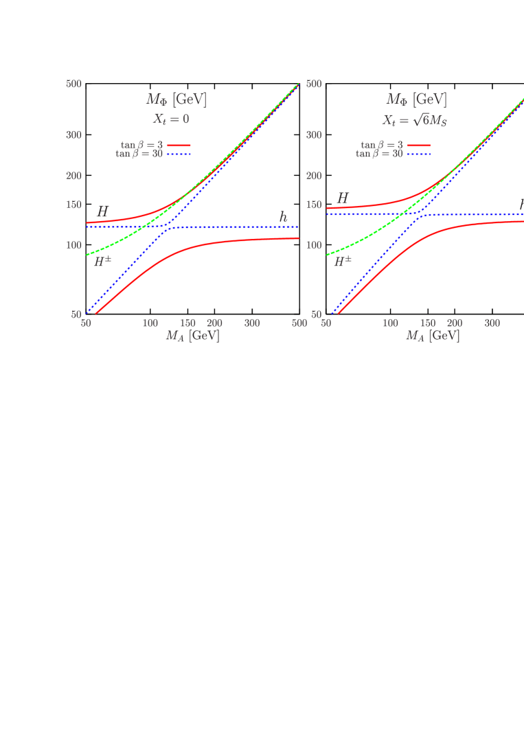
Figure 1: The masses of the MSSM Higgs bosons as a function of $M_{A}$ for two values $\tan\beta=3$ and 30, in the no mixing (left) and maximal mixing (right) scenarios with $M_{S}=2$ TeV and all the other SUSY parameters set to 1 TeV. The full set of radiative corrections is included with the pole masses $m_{t}=178$ GeV, $m_{b}=4.88$ GeV and with $\alpha_{s}(M_{Z})=0.1172$.

The radiatively corrected masses of the neutral CP–even and the charged Higgs bosons are displayed in Fig. 1 as functions of $M_{A}$ for the values $\tan\beta=3$ and $30$. The scenarios of no–mixing with $X_{t}=0$ (left) and maximal mixing with $X_{t}=\sqrt{6}M_{S}$ (right) have been assumed. As can be seen, a maximal value for the lighter Higgs mass, $M_{h}\sim 135$ GeV, is obtained for large $M_{A}$ values in the maximal mixing scenario with $\tan\beta=30$; the mass value is almost constant if $\tan\beta$ is increased. For no stop mixing, or when $\tan\beta$ is small, $\tan\beta\raisebox{-3.69899pt}{~{}\shortstack{$<$ \\ [-0.07cm] $\sim$}}~{}3$, the upper bound on the $h$ boson mass is smaller by more than 10 GeV in each case and the combined choice $\tan\beta=3$ and $X_{t}=0$, leads to a maximal value $M_{h}^{\rm max}\sim 110$ GeV. Also for large $M_{A}$ values, the $A,H$ and $H^{\pm}$ bosons (the mass of the latter being almost independent of the stop mixing and $\tan\beta$) become degenerate in mass. In the opposite case, i.e. for a light pseudoscalar, $M_{A}\raisebox{-3.69899pt}{~{}\shortstack{$<$ \\ [-0.07cm] $\sim$}}~{}M_{h}^{\rm max}$, it is $M_{h}$ which is very close to $M_{A}$, and the mass difference is particularly small for large $\tan\beta$ values.

The squares of the renormalized Higgs couplings to gauge bosons and to isospin $\pm\frac{1}{2}$ fermions are displayed in Figs. 2, as functions of $M_{A}$ in the no and maximal mixing cases, respectively; the SUSY and SM parameters are chosen as in Fig. 1. One notices the very strong variation with $M_{A}$ and the different pattern for values above and below the critical value $M_{A}\simeq M_{h}^{\rm max}$.

For small $M_{A}$ values the $hVV$ couplings are suppressed, with the suppression being stronger with large values of $\tan\beta$. For values $M_{A}\raisebox{-3.69899pt}{~{}\shortstack{$>$ \\ [-0.07cm] $\sim$}}~{}M_{h}^{\rm max}$, the $hVV$ boson couplings tend to unity and reach the values of the SM Higgs couplings, $g_{hVV}=1$ for $M_{A}\gg M_{h}^{\rm max}$; these values are reached more quickly when $\tan\beta$ is large. The situation in the case of the heavier CP–even $H$ boson is just opposite: its couplings are close to unity for $M_{A}\raisebox{-3.69899pt}{~{}\shortstack{$<$ \\ [-0.07cm] $\sim$}}~{}M_{h}^{\rm max}$ [which in fact is very close to the minimal value of $M_{H}$, $M_{H}^{\rm min}\simeq M_{h}^{\rm max}$, in particular at large $\tan\beta$], while above this limit, the $H$ couplings to gauge bosons are strongly suppressed. Note that the mixing $X_{t}$ in the stop sector does not alter this pattern, its main effect being simply to shift the value of $M_{h}^{\rm max}$.

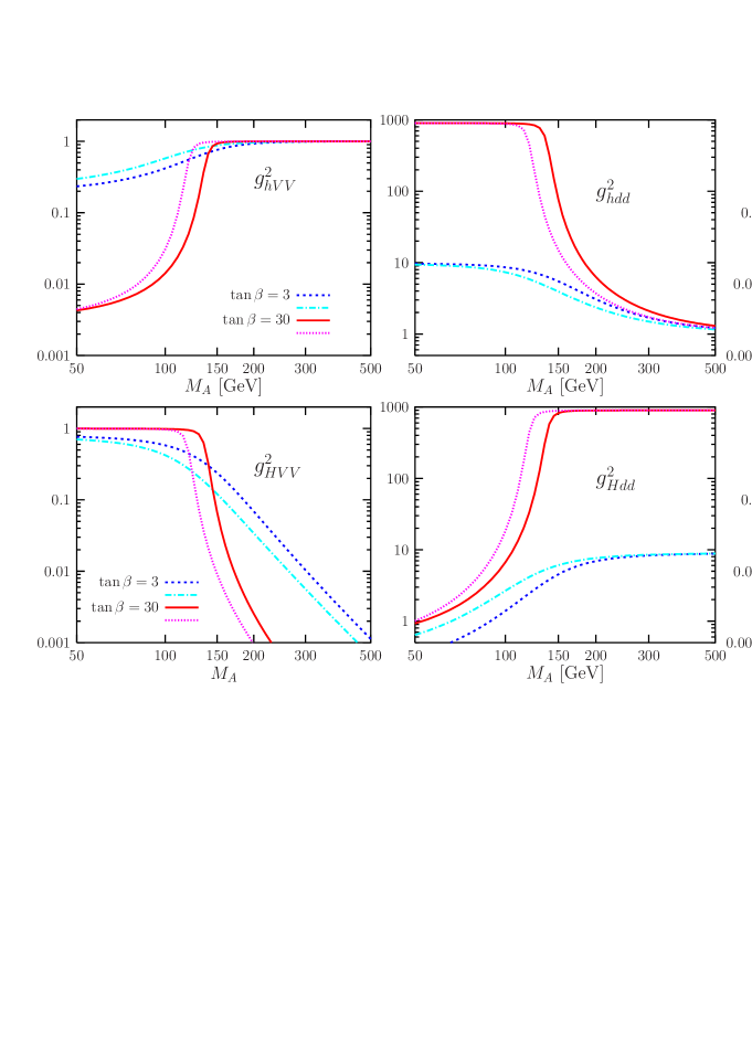
Figure 2: The normalized couplings squared of the CP–even MSSM neutral Higgs bosons to gauge bosons and fermions as a function of $M_{A}$ for $\tan\beta=3$ and 30 with the same inputs as in Fig. 1.

As in the case of the $VV$ couplings, there is a very strong variation of the Higgs couplings to fermions with $M_{A}$ and different behaviors for values above and below the critical mass $M_{A}\simeq M_{h}^{\rm max}$. For $M_{A}\raisebox{-3.69899pt}{~{}\shortstack{$<$ \\ [-0.07cm] $\sim$}}~{}M_{h}^{\rm max}$ the $h$ couplings to up–type fermions are suppressed, while those to down–type fermions are enhanced, with the suppression/enhancement being stronger at high $\tan\beta$. For $M_{A}\raisebox{-3.69899pt}{~{}\shortstack{$>$ \\ [-0.07cm] $\sim$}}~{}M_{h}^{\rm max}$, the normalized $h$ couplings tend to unity and reach the values of the SM Higgs couplings, $g_{hff}=1$, for $M_{A}\gg M_{h}^{\rm max}$; the limit being reached more quickly when $\tan\beta$ is large. The situation of the $H$ couplings to fermions is just opposite: they are close to unity for $M_{A}\raisebox{-3.69899pt}{~{}\shortstack{$<$ \\ [-0.07cm] $\sim$}}~{}M_{h}^{\rm max}$, while for $M_{A}\raisebox{-3.69899pt}{~{}\shortstack{$>$ \\ [-0.07cm] $\sim$}}~{}M_{h}^{\rm max}$, the couplings to up (down)–type fermions are suppressed (enhanced). For $M_{H}\gg M_{h}^{\rm max}$, they become approximately equal to those of the $A$ boson which couples to down (up)–type fermions proportionally to, respectively, $\tan\beta$ and $\cot\beta$. In fact, in this limit, also the $H$ coupling to gauge bosons approaches zero, i.e. as in the case of the $A$ boson.

Let us finally summarize the various regimes of the CP–conserving MSSM Higgs sector [19].

There is first the decoupling regime [46] for large values of $M_{A}$, which has been already mentioned. In this regime, which occurs in practice for $M_{A}\raisebox{-3.69899pt}{~{}\shortstack{$>$ \\ [-0.07cm] $\sim$}}~{}300$ GeV for low $\tan\beta$ and $M_{A}\raisebox{-3.69899pt}{~{}\shortstack{$>$ \\ [-0.07cm] $\sim$}}~{}M_{h}^{\rm max}$ for $\tan\beta\raisebox{-3.69899pt}{~{}\shortstack{$>$ \\ [-0.07cm] $\sim$}}~{}10$, the $h$ boson reaches its maximal mass value and its couplings to fermions and gauge bosons as well as its self–couplings become SM–like. The heavier $H$ boson has approximately the same mass as the $A$ boson and its interactions are similar, i.e. its couplings to gauge bosons almost vanish and the couplings to isospin $-\frac{1}{2}$ ($+\frac{1}{2}$) fermions are (inversely) proportional to $\tan\beta$. The $H^{\pm}$ boson is also degenerate in mass with the $A$ boson and its couplings to single $h$ bosons are suppressed. Thus, in the decoupling limit, the heavier Higgs bosons decouple and the MSSM Higgs sector reduces effectively to the SM Higgs sector, but with a light Higgs with a mass $M_{h}\raisebox{-3.69899pt}{~{}\shortstack{$<$ \\ [-0.07cm] $\sim$}}~{}140$ GeV. This light Higgs particle is nearly indistinguishable from the SM Higgs boson.

In the anti–decoupling regime [51], which occurs for a light pseudoscalar Higgs boson, $M_{A}\ll M_{h}^{\rm max}$, the situation is exactly opposite to the one of the decoupling regime. Indeed, in this case, the lighter tree–level $h$ mass is given by $M_{h}\simeq M_{A}|\cos 2\beta|$ while the tree–level heavier $H$ mass is given by $M_{H}\simeq M_{Z}(1+M_{A}^{2}\sin^{2}2\beta/M_{Z}^{2})$. At large values of $\tan\beta$, the $h$ boson is degenerate in mass with the $A$ boson, $M_{h}\simeq M_{A}$, while the $H$ boson has a mass close to its minimum which is in fact $M_{h}^{\rm max}\simeq\sqrt{M_{Z}^{2}+\epsilon}$. This is similar to the decoupling regime, except that the roles of the $h$ and $H$ bosons are reversed, and since there is an upper bound on $M_{h}$, all Higgs particles are light. Here, it is $\cos(\beta-\alpha)$ which is close to unity and $\sin(\beta-\alpha)$ which is small. Thus, it is the $h$ boson which has couplings close to those of the $A$ boson, while the $H$ boson couplings are SM–like.

The intense–coupling regime [52, 53] will occur when the mass of the pseudoscalar $A$ boson is close to $M_{h}^{\rm max}$. In this case, the three neutral Higgs bosons $h,H$ and $A$ [and even the charged Higgs particles] will have comparable masses, $M_{h}\sim M_{H}\sim M_{A}\sim M_{h}^{\rm max}$. The mass degeneracy is more effective when $\tan\beta$ is large. In this case both the $h$ and $H$ bosons have still enhanced couplings to down–type fermions and suppressed couplings to gauge bosons and up–type fermions.

The intermediate–coupling regime occurs for low values of $\tan\beta$, $\tan\beta\raisebox{-3.69899pt}{~{}\shortstack{$<$ \\ [-0.07cm] $\sim$}}~{}3$–5, and a not too heavy pseudoscalar Higgs boson, $M_{A}\raisebox{-3.69899pt}{~{}\shortstack{$<$ \\ [-0.07cm] $\sim$}}~{}300$–500 GeV [19]. Hence, we are not yet in the decoupling regime and both $\cos^{2}(\beta-\alpha)$ and $\sin^{2}(\beta-\alpha)$ are sizable, implying that both CP–even Higgs bosons have significant couplings to gauge bosons. The couplings between one gauge boson and two Higgs bosons, which are suppressed by the same mixing angle factors, are also significant. In addition, the couplings of the neutral Higgs bosons to down–type (up–type) fermions are not strongly enhanced (suppressed) since $\tan\beta$ is not too large.

Another possibility is the vanishing–coupling regime. For relatively large values of $\tan\beta$ and intermediate to large $M_{A}$ values, as well as for specific values of the other MSSM parameters entering the radiative corrections, there is a possibility of the suppression of the couplings of one of the CP–even Higgs bosons to fermions or gauge bosons, as a result of the cancellation between tree–level terms and radiative corrections [54]. In addition, in the case of the $hbb$ and $hgg$ couplings, a strong suppression might occur as a result of large direct corrections.

2.6 Constraints on the MSSM Higgs sector

There are various experimental constraints on the MSSM Higgs sector from the negative searches that have been performed up to now, mainly at LEP and Tevatron. They are summarized below.

At LEP, which has operated at energies up to 210 GeV, a 95% confidence level lower bound $M_{H_{\rm SM}}>114.4$ GeV has been set on the mass of the SM Higgs boson, by investigating the Higgs–strahlung process, $e^{+}e^{-}\to ZH_{\rm SM}$ [55, 56]. In the MSSM, this bound is valid for the lighter CP–even $h$ particle if its coupling to the $Z$ boson is SM–like $g^{2}_{ZZh}\simeq 1$ [i.e. almost in the decoupling regime] or in the case of the heavier $H$ particle if $g^{2}_{ZZH}\equiv\cos^{2}(\beta-\alpha)\simeq 1$ [i.e. in the anti–decoupling regime with a rather light $M_{A}$]. The complementary search of the neutral Higgs bosons in the associated production processes $e^{+}e^{-}\to hA$ and $HA$, allows to set the following combined 95% CL limits on the $h$ and $A$ boson masses [55, 56]

$$M_{h}>91.0~{}{\rm GeV}\ \ {\rm and}\ \ M_{A}>91.9~{}{\rm GeV}$$ (55)

[which apply only if the $b\bar{b}$ and $\tau\tau$ couplings of the $h/A$ states are not suppressed; see Ref. [58] e.g.] These bounds can be turned into exclusion regions in the MSSM parameter space. This is shown for the $\tan\beta$–$M_{h}$ plane in Fig. 3 where the no mixing (left) and maximal–mixing (right) scenarios are chosen with $M_{S}=1$ TeV and $m_{t}=174.3$ GeV [which is $1\sigma$ higher than the current experimental value $m_{t}\simeq 172$ GeV]; $\tan\beta$ is also allowed to be less than unity. As can be seen, with these specific assumptions, a significant portion of the parameter space is excluded for the maximal mixing scenario; values $\tan\beta\raisebox{-3.69899pt}{~{}\shortstack{$<$ \\ [-0.07cm] $\sim$}}~{}2$ are ruled out at the 95% CL. The exclusion regions are much larger in the no–mixing scenario since $M_{h}^{\rm max}$ is smaller by approximately 20 GeV and not far from the value that is experimentally excluded at LEP2 in the decoupling limit, $M_{h}\raisebox{-3.69899pt}{~{}\shortstack{$>$ \\ [-0.07cm] $\sim$}}~{}114.4$ GeV; for instance, the range $\tan\beta\raisebox{-3.69899pt}{~{}\shortstack{$<$ \\ [-0.07cm] $\sim$}}~{}5$ is excluded at 95% CL for $m_{t}=174.3$ GeV. The upper boundaries of the parameter space are indicated for other values of the top quark mass.

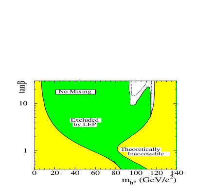
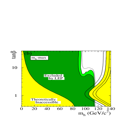
Figure 3: 95% CL contours in the $\tan\beta$–$M_{h}$ plane excluded by the negative searches of MSSM neutral Higgs bosons at LEP2 in the no–mixing (left) and maximal mixing (right) scenarios with $M_{S}=1$ TeV and $m_{t}=174.3$ GeV. The dashed lines indicate the boundaries that are excluded on the basis of a simulations in the absence of a signal; the upper boundaries of the parameter space are indicated for the values from left to right: $m_{t}=169.3,174.3,179.3$ and 183 GeV; from [56].

In the case of the charged Higgs boson, an absolute bound of $M_{H^{\pm}}\raisebox{-3.69899pt}{~{}\shortstack{$>$ \\ [-0.07cm] $\sim$}}~{}80$ GeV has been set by the LEP collaborations [56, 59] by investigating the pair production $e^{+}e^{-}\to H^{+}H^{-}$, with the $H^{\pm}$ bosons decaying into either $\nu\tau$ or $cs$ final states (see the next section). However, since in the MSSM, $M_{H^{\pm}}$ is constrained to be $M_{H^{\pm}}=\sqrt{M_{W}^{2}+M_{A}^{2}}$ and in view of the absolute bound on $M_{A}$, one should have $M_{H^{\pm}}\raisebox{-3.69899pt}{~{}\shortstack{$>$ \\ [-0.07cm] $\sim$}}~{}120$ GeV. The previous bound does not provide any additional constraint in the MSSM. A more restrictive bound is obtained from $H^{\pm}$ searches at the Tevatron in the decays of the heavy top quark, $t\rightarrow bH^{+}$ [60, 61], if $M_{H^{\pm}}\raisebox{-3.69899pt}{~{}\shortstack{$<$ \\ [-0.07cm] $\sim$}}~{}m_{t}-m_{b}\sim 170$ GeV (see also next section). However, the branching ratio compared to the dominant standard decay $t\rightarrow bW^{+}$, is large only for rather small, $\tan\beta\raisebox{-3.69899pt}{~{}\shortstack{$<$ \\ [-0.07cm] $\sim$}}~{}3$, and large, $\tan\beta\raisebox{-3.69899pt}{~{}\shortstack{$>$ \\ [-0.07cm] $\sim$}}~{}30$, values when the $H^{\pm}tb$ coupling is strongly enhanced. The outcome of the search is summarized in the right-hand side of Fig. 4 and as can be seen, it is only for $M_{H^{\pm}}\raisebox{-3.69899pt}{~{}\shortstack{$<$ \\ [-0.07cm] $\sim$}}~{}140$ GeV and $\tan\beta$ values below unity and above 60 (i.e. outside the theoretically favored $\tan\beta$ range in the MSSM) that the constraints are obtained [62].

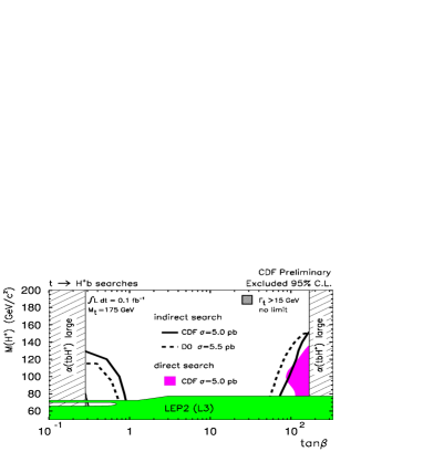
Figure 4: The constraint on $M_{H^{\pm}}$ as a function of BR$(H^{\pm}\to\tau\nu)$ from the negative searches of $H^{\pm}$ states by the ALEPH collaboration at LEP2 [59] (left) and the $\tan\beta$–$M_{H^{\pm}}$ parameter space excluded at the Tevatron from the non–observation of the top decay $t\to H^{+}b$ [62] (right).

2.7 Higgs bosons in non–minimal SUSY models

The Higgs sector in SUSY models may be slightly more complicated than the one of the CP–conserving MSSM discussed in the previous subsections. In the following, we briefly discuss the Higgs spectrum in some of these extensions and highlight the major differences with the MSSM.

In the presence of new sources of CP–violation in the SUSY sector, which is required if baryogenesis is to be explained at the electroweak scale, the new phases will enter the MSSM Higgs sector (which is CP–conserving at tree–level as discussed in one of the previous subsections) through the large radiative corrections which depend, for instance, on the parameters $A_{t}$ and $\mu$ that can involve complex phases in general. These corrections will affect the masses and the couplings of the neutral and charged Higgs particles. In particular, the three neutral Higgs bosons will not have definite CP quantum numbers and will mix with each other to produce the physical states $H_{1},H_{2}$ and $H_{3}$. The decay and production properties of the various Higgs particles can be significantly affected; for reviews, see e.g. Refs. [26, 27, 63]. Note, however, that there is a sum rule which forces the three $H_{i}$ bosons to share the coupling of the SM Higgs boson to gauge bosons, $\sum_{i}g_{H_{i}VV}^{2}=g^{2}_{H_{\rm SM}}$; only the CP–even component is projected out in these couplings.

An illustration of the Higgs mass spectrum is shown in Fig. 5 (left) as a function of the phase of the coupling $A_{t}$. As examples of new features compared to the usual MSSM, we simply mention the possibility of a relatively light $H_{1}$ state with very weak couplings to the gauge bosons. In this case, the cross section for $e^{+}e^{-}\to ZH_{1}$ is very small and if the states $H_{2},H_{3}$ are heavy, all Higgs particles can escape detection at LEP2 [64]. Another interesting feature is the possibility of resonant $H/A$ mixing when the two Higgs particles are degenerate in mass [26]. These features have to be proven to be a result of CP–violation.

   

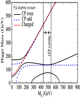
Figure 5: The spectrum of neutral Higgs particles in a CP–violating MSSM scenario (for $\tan\beta\!=\!5,M_{H^{\pm}}\!=\!150$ GeV and $M_{S}\!=\!0.5$ TeV) [27] (left) typical Higgs mass spectrum in the NMSSM as a function of $M_{A}$ [65] (center) and the upper bound on the lighter Higgs mass in a general SUSY model with an arbitrary number of doublets as a function of $\tan\beta$ [34].

The next–to–minimal SUSY extension, the NMSSM, in which the spectrum of the MSSM is extended by one singlet superfield, was among the first SUSY models based on supergravity-induced SUSY-breaking terms [14]. It has gained a renewed interest in the last decade, since it solves in a natural and elegant way the so-called $\mu$ problem [28] of the MSSM; in the NMSSM this parameter is linked to the vev of the singlet Higgs field (see Appendix), generating a $\mu$ value close to the SUSY-breaking scale. Furthermore, when the soft–SUSY breaking terms are assumed to be universal at the GUT scale, the model is very constrained as one single parameter allows to fully describe it [66]. The NMSSM leads to an interesting phenomenology as the MSSM spectrum is extended to include an additional CP-even and CP-odd Higgs states as well as a fifth neutralino, the singlino. An example of the Higgs mass spectrum [65] is shown in Fig. 5 (center). The upper bound on the mass of the lighter CP–even particle slightly exceeds that of the MSSM $h$ boson and the negative searches at LEP2 lead to looser constraints on the mass spectrum.

In a large area of the parameter space, the Higgs sector of the NMSSM reduces to the one of the MSSM but there is a possibility, which is not completely excluded, that is, one of the neutral Higgs particles, in general the lightest pseudoscalar $A_{1}$, is very light with a mass of a few ten’s of GeV. The light CP–even Higgs boson, which is SM–like in general, could then decay into pairs of $A_{1}$ bosons, $H_{1}\to A_{1}A_{1}\to 4b,4\tau$, with a large branching fraction. The possibility of having the CP–even $H_{1}$ state to be as light as $\sim 50$ GeV can also occur: being singlino–like, it will couple very weakly to $Z$ bosons and cannot be produced at LEP2. In this case, the SM–like Higgs boson is $H_{2}$ which would decay into pairs of $H_{1}$ states leading mostly to $4b$ jets, $H_{2}\to H_{1}H_{1}\to 4b$.

Higgs bosons in GUT theories. A large variety of theories, string theories, grand unified theories, left–right symmetric models, etc., suggest an additional gauge symmetry which may be broken only at the TeV scale. This leads to an extended particle spectrum and, in particular, to additional Higgs fields beyond the minimal set of the MSSM [31]. Especially common are new U(1)’ symmetries broken by the vev of a singlet field (as in the NMSSM) which lead to the presence of a $Z^{\prime}$ boson and one additional CP–even Higgs particle compared to the MSSM; this is the case, for instance, in the exceptional MSSM based on the string inspired $E_{6}$ symmetry. The secluded ${\rm SU(2)\times U(1)\times U(1)^{\prime}}$ model, in turn, includes four additional singlets that are charged under U(1)’, leading to 6 CP–even and 4 CP–odd neutral Higgs states. Other exotic Higgs sectors in SUSY models are, for instance, Higgs representations that transform as SU(2) triplets or bi–doublets under the ${\rm SU(2)_{L}}$ and ${\rm SU(2)_{R}}$ groups in left–right symmetric models, that are motivated by the seesaw approach to explain the small neutrino masses and which lead e.g. to a doubly charged Higgs boson $H^{--}$ [32, 33]. These extensions, which also predict extra matter fields, would lead to a very interesting phenomenology and new collider signatures in the Higgs sector.

In a general SUSY model, one can use an arbitrary number of isosinglet and isodoublet scalar fields to break the electroweak symmetry, while keeping the parameter $\rho=M_{W}^{2}/(\cos^{2}\theta_{W}M_{Z}^{2})$ naturally equal to unity at the tree level as it has been verified experimentally [55] (this is not the case of higher representations such as triplets without finetuning the vevs). However, in this case, one would need an extended matter content to allow for the unification of the three gauge couplings at the GUT scale. In this general model, a linear combination of Higgs fields has to generate the $W/Z$ masses and thus, from the triviality argument (which tells us that in the SM, the Higgs mass should be small if the model has to be extended to the GUT scale while leaving the quartic Higgs couplings finite), a Higgs particle should have a mass below 200 GeV and significant couplings to gauge bosons [34]. The upper bound on the mass of the lightest Higgs boson in this most general SUSY model is displayed in Fig. 5 (right) as a function of $\tan\beta$. This tell us that in supersymmetric theories, even in the most general case, a Higgs boson should be relatively light.

R–parity violating models. in which R–parity is spontaneously broken (and where one needs to either enlarge the SM symmetry or the spectrum to include additional gauge singlets), allow for an explanation of the light neutrino data [67]. Since R–parity breaking entails the breaking of the total lepton number $L$, one of the CP–odd scalars, the Majoron $J$, remains massless being the Goldstone boson associated to $L$ breaking. In these models, the neutral Higgs particles have also reduced couplings to the gauge bosons. More importantly, the CP–even Higgs particles can decay into pairs of invisible Majorons, $H_{i}\to JJ$, while the CP–odd particle can decay into a CP–even Higgs and a Majoron, $A_{i}\to H_{i}J$, and three Majorons, $A\to JJJ$ [67]. In the decoupling regime, only $H_{1}$ is light and one would have only one accessible Higgs boson which decays invisibly.

3 Decays of and into SUSY Higgs bosons

In this section, we discuss the various decay modes of the Higgs particles of the CP–conserving MSSM. We first assume that the SUSY particles are very heavy and do not affect the decay patterns and then, summarize the impact of light SUSY particles for both loop and direct decays. The decays of some SUSY particles into the MSSM Higgs bosons and the top quark decay into charged Higgs bosons will also be briefly discussed. But firstly, let us summarize the decay pattern of the SM Higgs particle, which can serve as a benchmark to be confronted later with the MSSM.

3.1 Decays of the SM Higgs boson

In the Standard Model, since the mass of the single Higgs boson $H$ is the only free parameter of the theory, the profile is uniquely determined once this parameter is fixed. In particular, the Higgs boson partial decay widths into the various final states and their branching fractions are fixed as the Higgs coupling to the particles are simply proportional to their masses. The decay modes [68, 69] their branching ratios and the total Higgs decay width are summarized in Fig. 6, which is obtained using the Fortran code HDECAY [70] mainly based on the work of Ref. [71]. The pole quark mass values, $m_{t}=172$ GeV, $m_{b}=4.9$ GeV and $m_{c}=1.64$ GeV and $\alpha_{S}=0.117$ have been used as inputs [55]. The most important radiative corrections have been included, in particular the QCD corrections to Higgs decays into quark pairs, the bulk of which can be mapped into running $\overline{\rm MS}$ quark masses defined at the scale $M_{H}$; the generally small electromagnetic and weak corrections are also incorporated. In addition, the QCD corrections to the loop decay modes into gluons and photons are included. Finally, below threshold three body decays into $WW^{*},ZZ^{*}$ and $\bar{t}t^{*}$ final states are implemented (in fact, the double off–shell decays of the massive gauge bosons which then decay into massless fermions $H\!\to\!V^{*}V^{*}\!\to\!4f$ are incorporated); see Ref. [71]

In the “low mass” range, 100 GeV $\raisebox{-3.69899pt}{~{}\shortstack{$<$ \\ [-0.07cm] $\sim$}}~{}M_{H}\raisebox{-3.69899pt}{~{}\shortstack{$<$ \\ [-0.07cm] $\sim$}}~{}130$ GeV, the main decay mode of the SM Higgs boson is by far $H\rightarrow b\bar{b}$ with a branching ratio of $\sim\,$75–50% for $M_{H}=115$–130 GeV, followed by the decays into $\tau^{+}\tau^{-}$ and $c\bar{c}$ pairs with branching ratios of the order of $\sim$ 7–5% and $\sim$ 3–2%, respectively. Also of significance is the $H\to gg$ decay with a branching fraction of $\sim\,$7% for $M_{H}\sim 120$ GeV. The $\gamma\gamma$ and $Z\gamma$ decays are rare, with branching ratios at the level of a few per mille, while the decays into pairs of muons and strange quarks (where $\bar{m}_{s}(1~{}{\rm GeV})=0.2$ GeV is used as input) are at the level of a few times $10^{-4}$. The $H\to WW^{*}$ decays, which are below the 1% level for $M_{H}\sim 100$ GeV, dramatically increase with $M_{H}$ to reach $\sim 30\%$ at $M_{H}\sim 130$ GeV; for this mass value, the mode $H\to ZZ^{*}$ occurs at the percent level.

In the “intermediate mass” range, $130\raisebox{-3.69899pt}{~{}\shortstack{$<$ \\ [-0.07cm] $\sim$}}~{}M_{H}\raisebox{-3.69899pt}{~{}\shortstack{$<$ \\ [-0.07cm] $\sim$}}~{}180$ GeV, the Higgs decays mainly into $WW$ and $ZZ$ pairs, with one virtual gauge boson below the $2M_{V}$ thresholds. The only other decay mode which survives is the $b\bar{b}$ decay which has a branching ratio that drops from 50% at $M_{H}\sim 130$ GeV to the level of a few percent for $M_{H}\sim 2M_{W}$. The $WW$ decay starts to dominate at $M_{H}\sim 130$ GeV and becomes gradually overwhelming, in particular for $2M_{W}\raisebox{-3.69899pt}{~{}\shortstack{$<$ \\ [-0.07cm] $\sim$}}~{}M_{H}\raisebox{-3.69899pt}{~{}\shortstack{$<$ \\ [-0.07cm] $\sim$}}~{}2M_{Z}$ where the $W$ boson is real (and thus $H\to WW$ occurs at the two–body level) while the $Z$ boson is still virtual, strongly suppressing the $H\to ZZ^{*}$ mode and leading to a $WW$ rate of almost 100%.

In the “high mass” range, $M_{H}\raisebox{-3.69899pt}{~{}\shortstack{$>$ \\ [-0.07cm] $\sim$}}~{}2M_{Z}$, the Higgs boson decays exclusively into the massive gauge boson channels with a branching ratio of $\sim 2/3$ for $WW$ and $\sim 1/3$ for $ZZ$ final states, slightly above the $ZZ$ threshold. The opening of the $t\bar{t}$ channel for $M_{H}\raisebox{-3.69899pt}{~{}\shortstack{$>$ \\ [-0.07cm] $\sim$}}~{}350$ GeV does not alter significantly this pattern, in particular for high Higgs masses: the $H\to t\bar{t}$ branching ratio is at the level of 20% slightly above the $2m_{t}$ threshold and starts decreasing for $M_{H}\sim 500$ GeV to reach a level below 10% at $M_{H}\sim 800$ GeV. The reason is that while the $H\to t\bar{t}$ partial decay width grows as $M_{H}$, the partial decay width into (longitudinal) gauge bosons increases as $M_{H}^{3}$.

Finally, for the total decay width, the Higgs boson is very narrow in the low mass range, $\Gamma_{H}<10$ MeV, but the width becomes rapidly wider for masses larger than 130 GeV, reaching $\sim 1$ GeV slightly above the $ZZ$ threshold. For larger Higgs masses, $M_{H}\raisebox{-3.69899pt}{~{}\shortstack{$>$ \\ [-0.07cm] $\sim$}}~{}500$ GeV, the Higgs boson becomes obese: its decay width is comparable to its mass because of the longitudinal gauge boson contributions in the decays $H\to WW,ZZ$. For $M_{H}\sim 1$ TeV, one has a total decay width of $\Gamma_{H}\sim 700$ GeV, resulting in a very broad resonant structure.

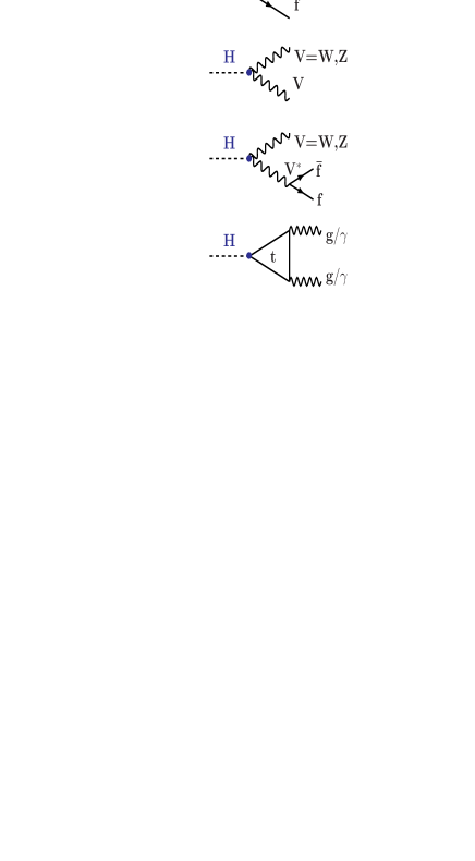
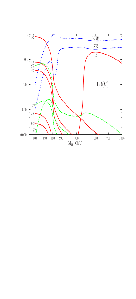
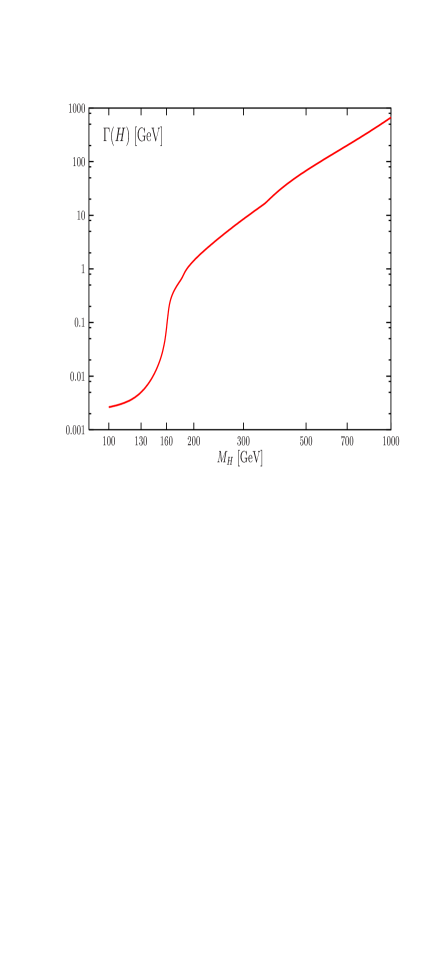
Figure 6: The main decay processes (left), the branching ratios (center) and the total decay width (right) of the SM Higgs boson as a function of its mass, as obtained with HDECAY [70].

3.2 Decays of the MSSM Higgs bosons

In the decoupling regime, $M_{A}\raisebox{-3.69899pt}{~{}\shortstack{$>$ \\ [-0.07cm] $\sim$}}~{}150$ GeV for $\tan\beta=30$ and $M_{A}\raisebox{-3.69899pt}{~{}\shortstack{$>$ \\ [-0.07cm] $\sim$}}~{}400$–500 GeV for $\tan\beta=3$, the situation is quite simple; Fig. 7. The lighter $h$ boson reaches its maximal mass value and has SM–like couplings and, thus, decays as the SM Higgs boson discussed previously. Since $M_{h}^{\rm max}\raisebox{-3.69899pt}{~{}\shortstack{$<$ \\ [-0.07cm] $\sim$}}~{}130$ GeV, the dominant modes are the decays into $b\bar{b}$ pairs and into $WW^{*}$ final states, the branching ratios being of the same size in the upper mass range. The decays into $\tau^{+}\tau^{-},gg,c\bar{c}$ and also $ZZ^{*}$ final states are at the level of a few percent and the loop induced decays into $\gamma\gamma$ and $Z\gamma$ at the level of a few per mille. The total decay width of the $h$ boson is small, $\Gamma(h)\raisebox{-3.69899pt}{~{}\shortstack{$<$ \\ [-0.07cm] $\sim$}}~{}{\cal O}$(10 MeV).

For the heavier Higgs bosons, the decay pattern depends on $\tan\beta$. For $\tan\beta\gg 1$, as a result of the strong enhancement of the couplings to down–type fermions, the $H$ and $A$ bosons will decay almost exclusively into $b\bar{b}$ ($\sim 90\%$) and $\tau^{+}\tau^{-}$ ($\sim 10\%)$ pairs; the $t\bar{t}$ decay when kinematically allowed and all other decays, including the $H\to VV^{(*)}$ modes, are strongly suppressed. The $H^{\pm}$ boson decays mainly into $tb$ pairs but there is also a a significant fraction of $\tau\nu_{\tau}$ final states ($\sim 10\%$). For low values of $\tan\beta$, the decays of the neutral Higgs bosons into $t\bar{t}$ pairs and the decays of the charged Higgs boson in $tb$ final states are by far dominating. For intermediate values, $\tan\beta\sim 10$, the rates for the $H,A\to b\bar{b}$ and $t\bar{t}$ decays are comparable, while the $H^{\pm}\to\tau\nu$ decay stays at the 10% level. For small and large $\tan\beta$ values, the total decay widths of the four Higgs bosons are, respectively, of ${\cal O}$(1 GeV) and of ${\cal O}$(10 GeV) and thus not large. This is because the decay modes into $W$ and $Z$ bosons are absent or strongly suppressed, contrary to the SM case.

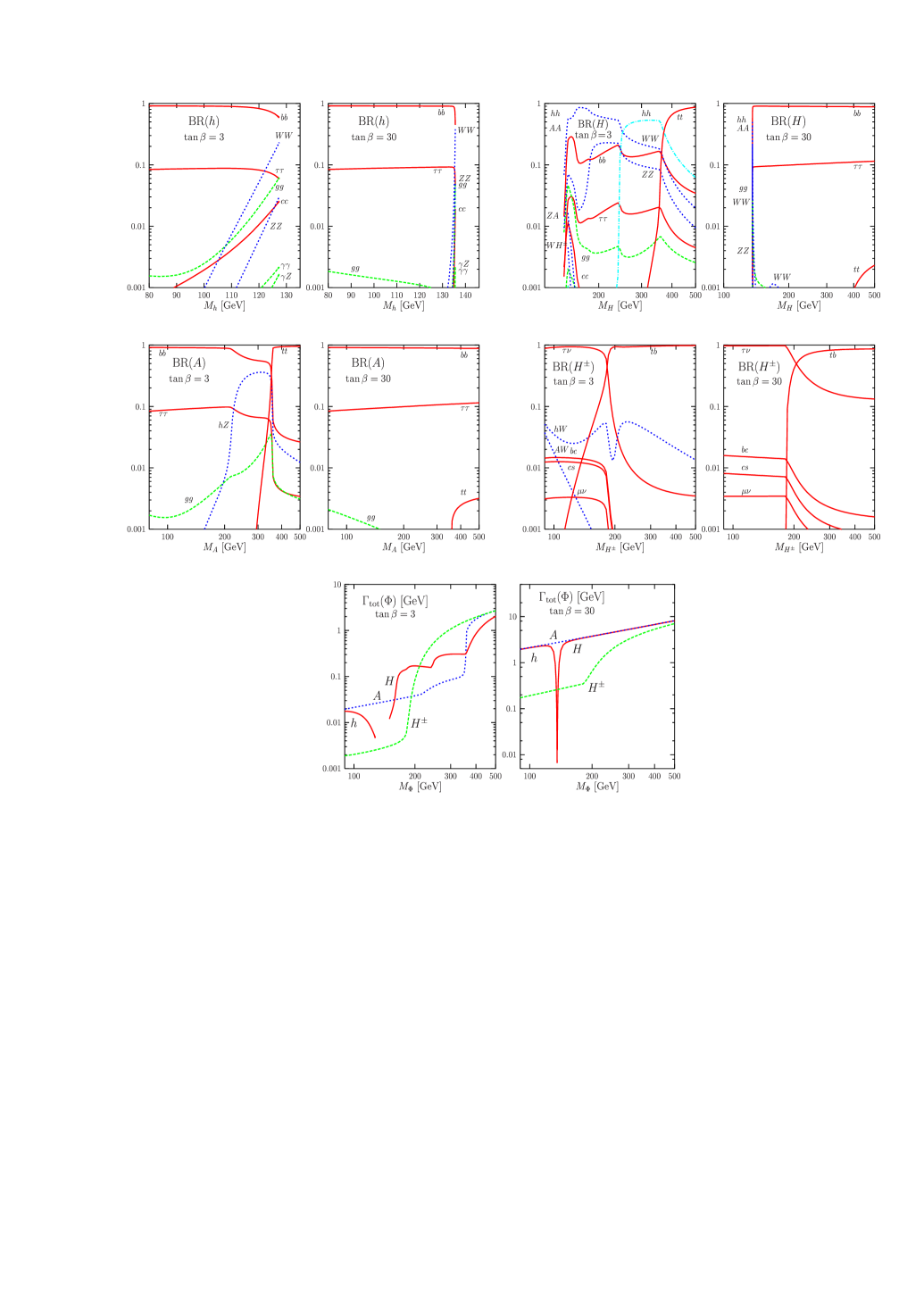
Figure 7: The decay branching ratios and total widths of the MSSM Higgs bosons as functions of their masses for $\tan\beta=3,30$ in the maximal mixing scenario as obtained with HDECAY [70] with the inputs of Fig. 1; the radiative corrections [50] and the three-body decays are included.

Outside the decoupling regime, the decay pattern can be summarized as follows:

– In the anti–decoupling regime, i.e. when $\tan\beta\raisebox{-3.69899pt}{~{}\shortstack{$>$ \\ [-0.07cm] $\sim$}}~{}10$ and $M_{A}\raisebox{-3.69899pt}{~{}\shortstack{$<$ \\ [-0.07cm] $\sim$}}~{}M_{h}^{\rm max}$, the pattern for the Higgs decays is also rather simple. The $h$ and $A$ bosons will mainly decay into $b\bar{b}$ ($\sim 90\%$) and $\tau^{+}\tau^{-}$ ($\sim 10\%)$ pairs, while the charged $H^{\pm}$ boson decays almost all the time into $\tau\nu_{\tau}$ pairs ($\sim 100\%)$. All other modes are suppressed down to a level below $10^{-3}$ except for the gluonic decays of $h$ and $A$ [in which the $b$–loop contributions are enhanced by the same $\tan\beta$ factor] and some fermionic decays of $H^{\pm}$. Although their masses are small, the three Higgs bosons have relatively large total widths, $\Gamma(h,A,H^{\pm})\sim{\cal O}$(1 GeV) for $\tan\beta=30$. The heavier $H$ boson will play the role of the SM Higgs boson, but with one major difference: in the low $M_{A}$ range (which is now excluded by LEP2 searches), the $h$ and $A$ particles are light enough for the two–body decays $H\to hh$ and $H\to AA$ to take place and to dominate with a branching fraction of $\sim 50\%$ each. These decays can be very important in some extensions such as the CP–violating MSSM and the NMSSM.

– In the intense–coupling regime, with $\tan\beta\raisebox{-3.69899pt}{~{}\shortstack{$>$ \\ [-0.07cm] $\sim$}}~{}10$ and $M_{A}\sim 100$–140 GeV, the couplings of both $h$ and $H$ to gauge bosons and up–type fermions are suppressed and those to down–type fermions are enhanced. Because of this enhancement, the branching ratios of the $h$ and $H$ bosons to $b\bar{b}$ and $\tau^{+}\tau^{-}$ final states are the dominant ones, with values as in the pseudoscalar Higgs case, i.e. $\sim 90$% and $\sim 10$%, respectively. The interesting rare decay mode into $\gamma\gamma$ is very strongly suppressed for the three neutral Higgs particles compared to the SM. The branching ratios for the decays into muons, which are not displayed in Fig. 7 are at the level of $3\times 10^{-4}$. The $H^{\pm}$ boson in this scenario decays mostly into $\tau\nu$ final states.

– In the intermediate–coupling regime, i.e. for $\tan\beta\!\sim\!3$ and $H/A$ masses below the $t\bar{t}$ threshold, interesting decays of the $H,A$ and $H^{\pm}$ bosons occur. For the pseudoscalar $A$, the decay $A\to hZ$ is dominant when kinematically accessible, i.e. for $M_{A}\raisebox{-3.69899pt}{~{}\shortstack{$>$ \\ [-0.07cm] $\sim$}}~{}200$ GeV, with a branching ratio exceeding the 50% level. In the case of $H$, the channel $H\to hh$ is very important, reaching the level of 60% in a significant $M_{H}$ range; the decays into weak vector bosons and $b\bar{b}$ pairs are also significant. For the $H^{\pm}$ boson, the interesting decay $H^{\pm}\to hW^{\pm}$ is at the level of a few percent while the other decay $H^{\pm}\to AW^{\pm}$ is kinematically challenged and occurs at the three–body level.

– Finally, for the choice of input SUSY parameters of Fig. 7, the vanishing coupling regime does not occur. However, when Higgs couplings to bottom quarks and $\tau$ leptons accidentally vanish, the outcome is rather clear. For the $h$ boson for instance, the $WW^{*}$ mode becomes the dominant one, followed by the loop induced $h\to gg$ decay; the interesting $h\to\gamma\gamma$ decay mode is enhanced but stays below the permille level.

3.3 The impact of light SUSY particles

In the preceeding discussion, we have assumed that the SUSY particles are too heavy to substantially contribute to the loop induced decays of the neutral Higgs bosons and to the radiative corrections to the tree–level decays. In addition, we have ignored the Higgs decay channels into sparticles which were considered as being kinematically shut. However, some SUSY particles such as the charginos, neutralinos and possibly sleptons and third generation squarks, could be light enough to play a significant role in this context. We thus summarize their possible impact.

In the case of Higgs decays into $b$ quarks, besides the radiative corrections to the Higgs masses and the angle $\alpha$, there are large direct corrections, eq. (53). The corrections generate a strong variation of the $b\bar{b}$ partial widths of the three neutral Higgs bosons which can reach the level of 50% for large $\mu$ and $\tan\beta$ values, and not too heavy squarks and gluinos. However, they have only a small impact on the $b\bar{b}$ rates since these decays dominate in general. In turn, they can have a large influence on the rates for the other decay modes, in particular, on the $\tau^{+}\tau^{-}$ channels. This can be seen in Fig. 8 (left) where the rates of $h,H,A$ decays into $b\bar{b}$ and $\tau^{+}\tau^{-}$ are shown for $\tan\beta=30$; variations of BR$(\tau^{+}\tau^{-})$ by a factor of two can be noticed. In the case of the $H,A$ bosons with masses above the $t\bar{t}$ threshold and for intermediate $\tan\beta$ values when the $b\bar{b}$ and $t\bar{t}$ channels compete with each other, these corrections can be felt by both the $H/A\to b\bar{b}$ and $t\bar{t}$ rates. The same features occur in the case of the $H^{\pm}$ boson decaying into $tb$ and $\tau\nu$ final states.

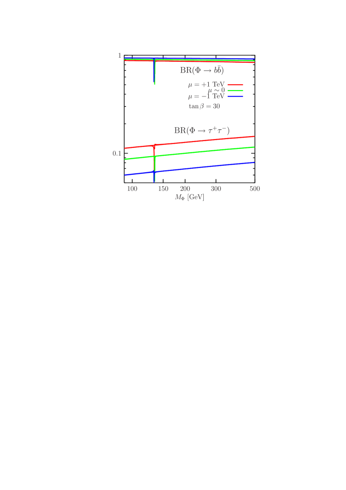
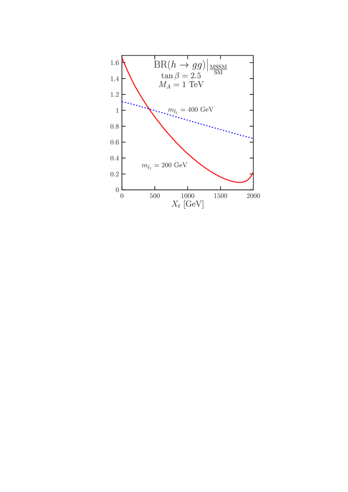
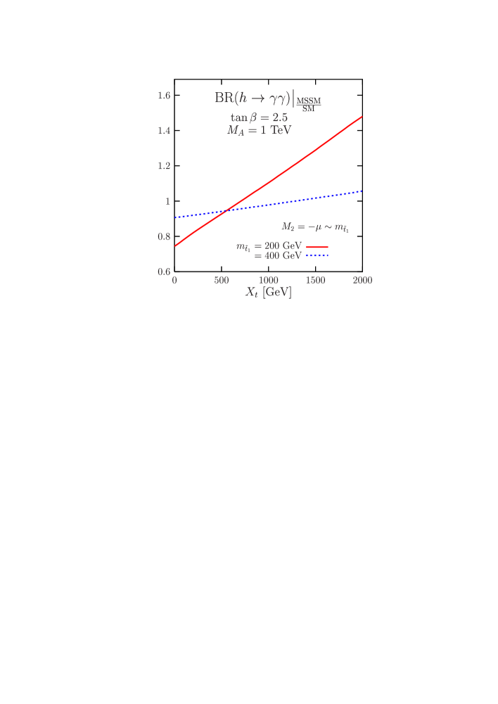
Figure 8: The branching ratios: for $h,A,H\to b\bar{b}$ and $\tau^{+}\tau^{-}$ for $\tan\beta=30$ with/without the SUSY–QCD corrections [19] (left) and for the gluonic (center) and photonic (right) decays of the $h$ boson in the decoupling limit relative to their SM values including SUSY loops with $\tan\beta=2.5$ [72].

If squarks are relatively light, they can lead to sizable contributions to the loop induced decays $h,H\to gg$ and $\gamma\gamma$; due to CP–invariance which forbids $A$ couplings to identical $\tilde{q}_{i}\tilde{q}_{i}$ states, squark loops do not contribute to $A\to gg,\gamma\gamma$. Since squarks have Higgs couplings that are not proportional to their masses, their contributions are damped by loop factors $1/m_{\tilde{Q}}^{2}$ and, contrary to SM quarks, the contributions become very small at high $m_{\tilde{Q}}$ and the sparticles decouple completely from the vertices. However, when $m_{\tilde{Q}}\sim M_{h,H}$, the contributions can be significant [72]. This is particularly true in the case of top squarks in the decays $h\to gg$, the reason being two–fold: $(i)$ the $\tilde{t}$ mixing, $\propto m_{t}X_{t}$, can be very large and could lead to $\tilde{t}_{1}$ that is much lighter than all other squarks and even the top quark, and $(ii)$ the coupling of top squarks to the $h$ boson involves a component which is proportional to $m_{t}X_{t}$ and for large $A_{t}$, it can be strongly enhanced. Sbottom mixing, $\propto m_{b}X_{b}$, can also be sizable for large $\tan\beta$ and $\mu$ values and can lead to light $\tilde{b}_{1}$ states with strong couplings to the $h$ boson. Besides, chargino loops enter also the $h,H,A\to\gamma\gamma$ decays but their contributions is in general smaller since the Higgs$\chi\chi$ couplings are not strongly enhanced.

Figure 8 shows the deviations of the gluonic and photonic widths of the $h$ boson, relative to their SM values, as a result of $\tilde{t}$ contributions. In the case of $h\to gg$, the partial width can be reduced by an order of magnitude for light stops and large $X_{t}$ mixing. For the $h\gamma\gamma$ coupling, as the interference can be either positive or negative, the rate can be increased by more than 50% or slightly suppressed. Chargino loops in $h\gamma\gamma$ contribute less than 10%. Note that for the $Hgg$ and $H\gamma\gamma$ couplings, SUSY effects might be larger as the $H$ boson and loop masses can be comparable; however, in this case, both the photonic and gluonic branching ratios are too small.

Let us now turn to decays of the MSSM Higgs bosons into SUSY particles [17, 73, 74, 75] and start with decays into charginos and neutralinos, collectively called inos. The sum of the branching ratios for the Higgs decays into all possible combinations of ino states are shown in Fig. 9 as a function of the Higgs masses for the values $\tan\beta\!=\!3,30$ for $H,A$ and $H^{\pm}$ and $\tan\beta\!=\!10$ for $h$. To allow for such decays, we have departed from the benchmark of Fig.1, to adopt a scenario in which we have still $M_{S}=2$ TeV with maximal stop mixing, but where the parameters in the gaugino sector are $M_{2}\!=\!-\mu=150$ GeV. Here, the universality of the gaugino masses at the GUT scale, giving $M_{2}\sim 2M_{1}$ at low scales, is assumed while $M_{3}$ is still large. This choice leads to rather light ino states, $m_{\chi_{i}}\raisebox{-3.69899pt}{~{}\shortstack{$<$ \\ [-0.07cm] $\sim$}}~{}200$–250 GeV which still satisfy the LEP bound, $m_{\chi_{1}^{\pm}}\raisebox{-3.69899pt}{~{}\shortstack{$>$ \\ [-0.07cm] $\sim$}}~{}100$ GeV [55].

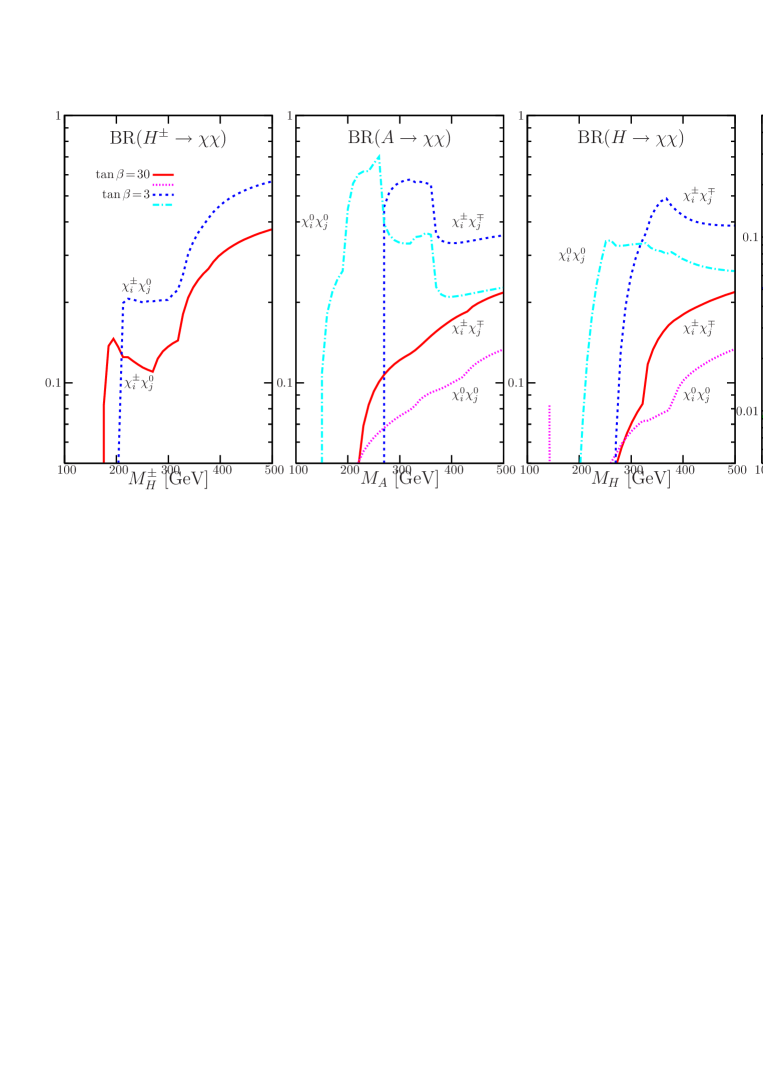
Figure 9: The branching ratios for the MSSM $H,A,H^{\pm}\,(h)$ decays into the sum of charginos and/or neutralinos as a function of their masses for $\tan\beta\!=\!3,30(10)$ [19]. The relevant SUSY parameters are $M_{S}=2$ TeV and $M_{2}\!=\!-\!\mu\!=\!150$ GeV and for $h$, the relation $M_{2}\!\sim\!2M_{1}$ is relaxed.

In general, for the heavy $H,A,H^{\pm}$ states, the sum of these branching ratios is always large except in a few cases: ($i$) for small $M_{A}$ when the phase space is too penalizing and does not allow for the decay into (several) inos to occur; $(ii$) for the $H$ boson in the mass range $M_{H}\sim 200$–350 GeV and small $\tan\beta$ values when the decay $H\rightarrow hh$ is largely dominant; and ($iii$) for $H^{\pm}$ just above the $t\bar{b}$ threshold if not all ino decay channels are open. In fact, even above the thresholds of Higgs decays into top quarks and/or large $\tan\beta$ values, the decays into inos can be important: for very heavy Higgs bosons, they reach a common value of $30\%$ for low $\tan\beta\sim 2$ and large $\tan\beta\sim 30$ and are dominant for moderate values $\tan\beta\sim 10$ when the Higgs–$b\bar{b}$ couplings are not yet strongly enhanced. Note that when kinematically open, neutral Higgs decays into charginos dominate over those into neutralinos, as the charged couplings are larger than the neutral ones.

The bound $m_{\chi_{1}^{\pm}}\raisebox{-3.69899pt}{~{}\shortstack{$>$ \\ [-0.07cm] $\sim$}}~{}100$ GeV does not allow for ino decay modes of the lightest $h$ boson since $M_{h}\raisebox{-3.69899pt}{~{}\shortstack{$<$ \\ [-0.07cm] $\sim$}}~{}140$ GeV, except for the invisible decays into a pair of the lightest neutralinos, $h\to\chi_{1}^{0}\chi_{1}^{0}$ [73, 74]. This is particularly true when the universality relation $M_{2}\sim 2M_{1}$ is relaxed leading to light LSPs while the bound on $m_{\chi_{1}^{\pm}}$ is respected [74]. In general, when the $h\to\chi_{1}^{0}\chi_{1}^{0}$ decay is kinematically allowed, the branching ratio is sizable only in the decoupling regime (where the $hbb$ couplings are not enhanced) and for mixed higgsino–gaugino states (which maximizes the $h\chi\chi$ couplings). Figure 9 (right) shows that the rate can exceed the 10% level in this case.

Another possible decay channel for the heavy $H,A,H^{\pm}$ bosons is into sfermions; for the $h$ boson, these decays are kinematically closed as $m_{\tilde{f}}\raisebox{-3.69899pt}{~{}\shortstack{$>$ \\ [-0.07cm] $\sim$}}~{}100$ GeV from LEP and Tevatron searches. The decays into first/second generation sfermions are marginal, as the Higgs couplings to these states are small, while those into third generation sfermions, can be more important [75]. For instance, $H$ decays into light top squarks can be significant and even dominant if the $H\tilde{t}_{1}\tilde{t}_{1}$ coupling is enhanced. Mixed $H,A\to\tilde{t}_{1}\tilde{t}_{2}$ and $H^{+}\tilde{t}_{1}\tilde{b}_{1}$ decays can also be significant when phase space allowed. Decays of the Higgs bosons into tau sleptons, which are more favored by phase space, can also be sizeable but they have to compete with decays into $b\bar{b}$ which are strongly enhanced at large $\tan\beta$. This is also the case for the decays involving $\tilde{b}$ squarks in the final state.

3.4 Decays of the sparticles and the top quark into Higgs bosons

Let us now briefly comment on a related issue which is the decays of SUSY particles into Higgs bosons [76, 77]. If the mass splitting between the heavier $\chi_{3,4}^{0},\chi_{2}^{\pm}$ chargino/neutralino states and the lighter $\chi_{1,2}^{0},\chi_{1}^{\pm}$ states is substantial, the heavier inos can decay into the lighter ones and neutral and/or charged Higgs bosons, $\chi_{2}^{\pm},\chi_{3}^{0},\chi_{4}^{0}\to\chi_{1}^{\pm},\chi_{2}^{0},\chi_{1}^{0}+h,H,A,H^{\pm}$. In fact, even the next–to–lightest neutralino can decay into the LSP neutralino and a neutral Higgs boson and the lighter chargino into the LSP and a charged Higgs boson, $\chi_{2}^{0}\to\chi_{1}^{0}+h,H,A$ and $\chi_{1}^{\pm}\to\chi_{1}^{0}+H^{\pm}$.

These decay processes will be in direct competition with decays into gauge bosons and, if sleptons/squarks are light, decays into sfermions and fermion partners. The decay branching ratios of the heavier $\chi_{2}^{\pm}$ and $\chi_{3}^{0}$ states into the lighter ones $\chi_{1}^{\pm}$ and $\chi_{1,2}^{0}$ and Higgs bosons are shown in Fig. 10 for $\tan\beta=10$ and $M_{A}=180$ GeV with $\mu=150$ GeV, which means that the lighter inos are higgsino like. The other parameter $M_{2}$ is varied with the mass of the decaying ino. Sleptons and squarks are assumed to be too heavy to play a role here. Since the Higgs bosons couple preferentially to mixtures of gauginos and higgsinos, the couplings to mixed heavy and light chargino/neutralino states are maximal. To the contrary, the gauge boson couplings to inos are important only for higgsino– or gaugino–like states. Thus, in principle, the (higgsino or gaugino–like) heavier inos $\chi_{2}^{\pm}$ and $\chi_{3,4}^{0}$ will dominantly decay, if phase space allowed, into Higgs bosons and the lighter $\chi$ states. As is usually the case, the charged current decay modes will be more important than the neutral modes. A similar pattern occurs for large values of $\mu$ compared to $M_{2}$ in which case the light (heavy) inos are gauginos (higgsinos).

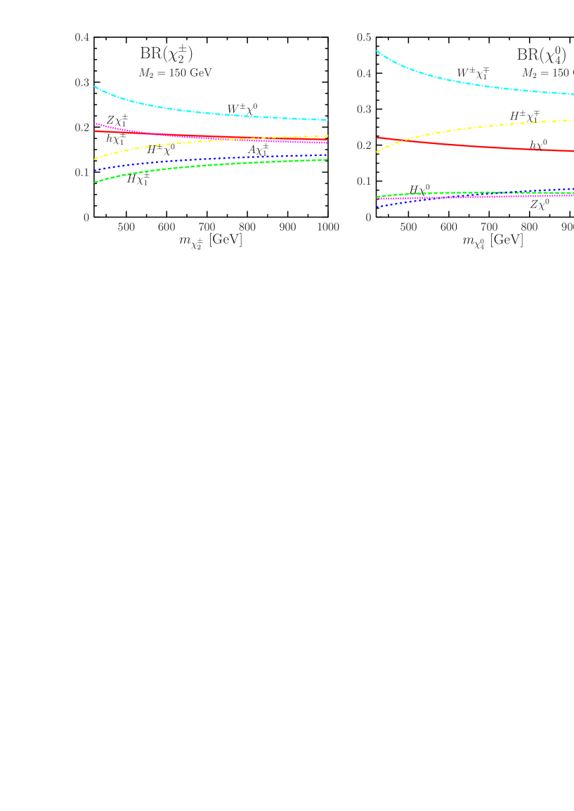
Figure 10: The branching ratios for the decays of $\chi_{2}^{\pm}$ and $\chi_{4}^{0}$ into Higgs and gauge bosons for $\tan\beta=10,M_{A}=180$ GeV and $\mu=150$ GeV, as a function of the ino masses and hence $M_{2}$ [77]. Similar features occur for the decays of $\chi_{3}^{0}$ and when $\mu$ and $M_{2}$ are interchanged.

Another potentially large source of Higgs bosons comes from the decays of sfermions [75]. If the mass splitting between two squarks of the same generation is large enough, as is generally the case of the $(\tilde{t},\tilde{b})$ isodoublet, the heavier squark can decay into the lighter one plus a neutral or charged Higgs boson, a channel which will compete with the usually dominant modes into quarks and charginos or neutralinos. This is particularly the case for the $\tilde{t}_{2}\to\tilde{t}_{1}+h/H/A$ decays which can have a substantial rate for moderate to large $X_{t}$ values which enhance the Higgs–$\tilde{t}_{1}\tilde{t}_{2}$ coupling.

Finally, another important source of relatively light charged Higgs bosons, $M_{H^{\pm}}\raisebox{-3.69899pt}{~{}\shortstack{$<$ \\ [-0.07cm] $\sim$}}~{}m_{t}$, comes for the decays of the heavy top quark, $t\to H^{+}b$ [60]. The couplings of the $H^{\pm}$ bosons to $tb$ states are proportional to the combinations $m_{b}\tan\beta(1+\gamma_{5})+m_{t}{\rm cot}\beta(1-\gamma_{5})$. They are thus strong enough for small $\tan\beta\sim 1$ or large $\tan\beta\raisebox{-3.69899pt}{~{}\shortstack{$>$ \\ [-0.07cm] $\sim$}}~{}30$ values to make this decay compete with the standard $t\to bW^{+}$ channel, the only relevant mode otherwise. For intermediate values of $\tan\beta$, the $t\,(b)$–quark component of the coupling is suppressed (not too strongly enhanced yet) and the overall couplings is small; the minimal value occurs at $\tan\beta=\sqrt{m_{t}m_{b}}\sim 6$. The $t\to bH^{+}$ branching ratio is shown in Fig. 11 as a function of the $H^{\pm}$ mass for three values, $\tan\beta=3,10$ and 30. One notices the small value of the rate at intermediate $\tan\beta$, while it exceeds the level of a few percent for $\tan\beta=3$ and 30. There also a clear suppression near the threshold: for $M_{H^{\pm}}\raisebox{-3.69899pt}{~{}\shortstack{$>$ \\ [-0.07cm] $\sim$}}~{}160$ GeV, the branching ratio being below the per mille level even for $\tan\beta=3$ and $30$.

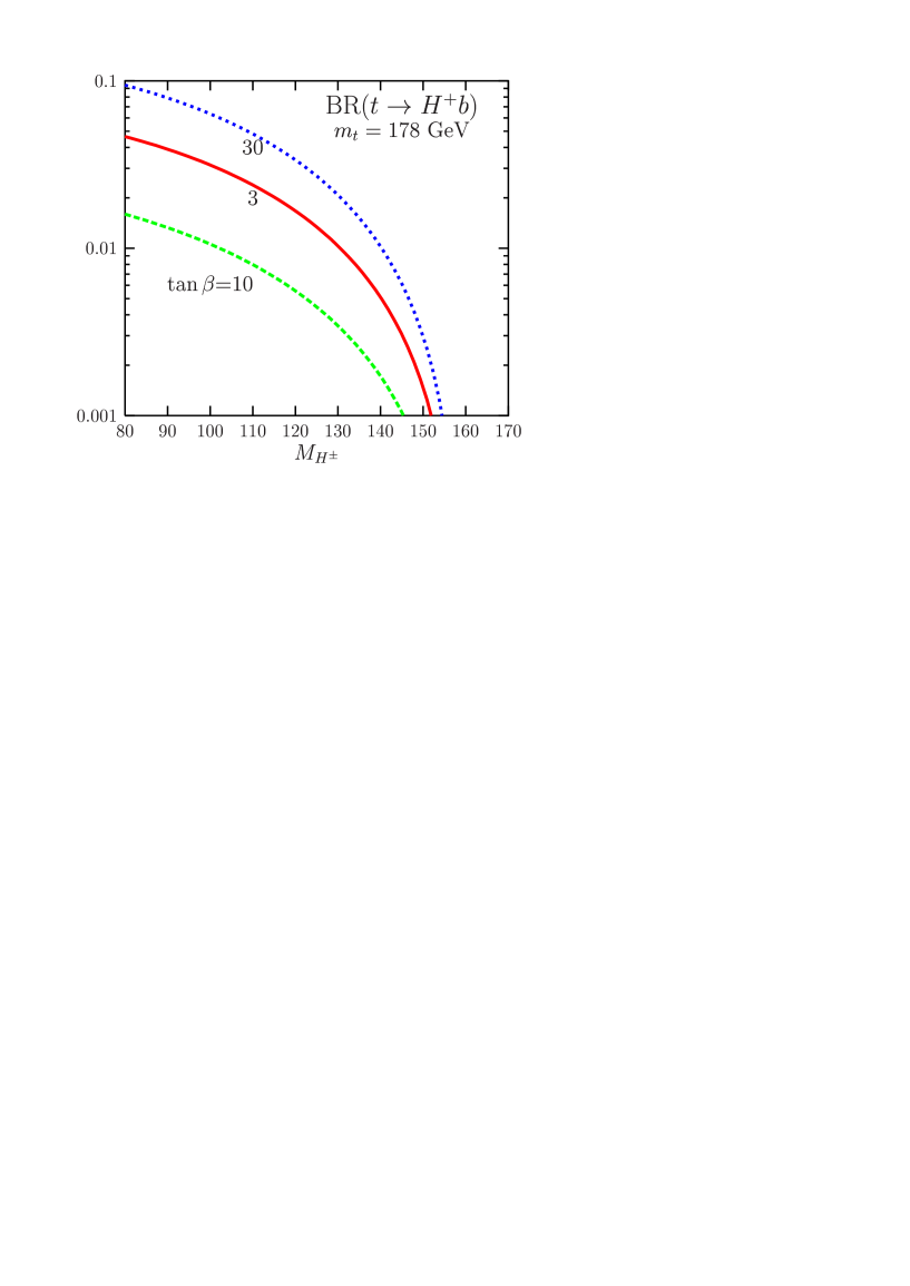
Figure 11: The branching ratio for the decay of the top quark into a charged Higgs boson and a bottom quark as a function of $M_{H^{\pm}}$ for three values $\tan\beta=3,10$ and 30.

4 SUSY Higgs production at the LHC

As in the previous section, we will first summarize the salient features of SM Higgs production at the LHC and then then discuss the main differences for MSSM Higgs production. We first assume that the SUSY particles are heavy and then emphasize impact of light SUSY particles.

4.1 Production of the SM Higgs particle

There are essentially four mechanisms for the single production of the SM Higgs boson at hadron colliders [80, 81, 82, 83], the Feynman diagrams of which are shown in the left-hand side of Fig. 12. The total production cross sections, as obtained with the Fortran programs of Ref. [84] and the SM inputs used for the Higgs decays in the SM, are displayed in the center of Fig. 12 for the LHC with a center of mass energy $\sqrt{s}=14$ TeV as a function of the Higgs mass. The MRST parton distributions functions [85] have been adopted and the next-to–leading order (NLO), and eventually the next-to-NLO (NNLO), radiative corrections have been implemented [18, 86, 87] as will be summarized later when the main features of each production channel will be discussed. The significance for detecting the Higgs particle in the various production and decay channels is shown in the right-hand side of Fig. 12, assuming a 100 fb^-1 integrated luminosity.

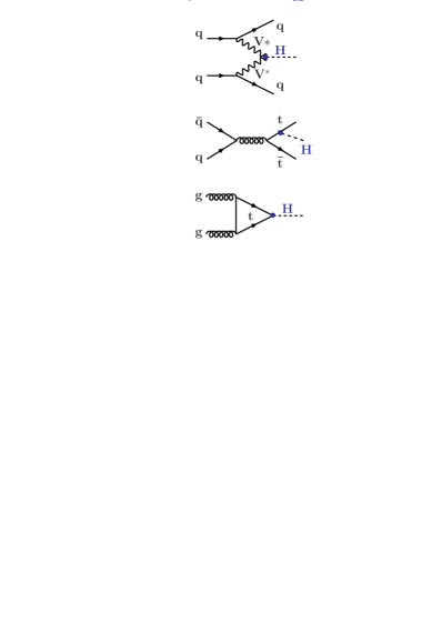
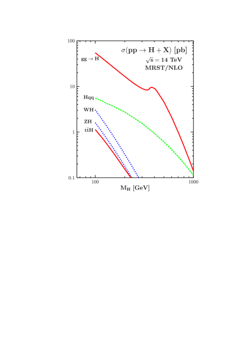
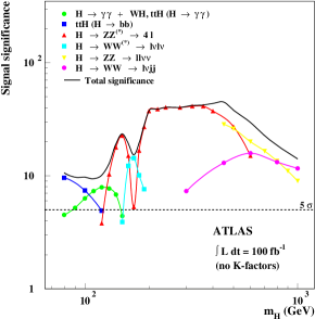
Figure 12: The dominant production mechanisms (left), the total production cross sections (center) and the significance for the experimental detection [37] (right) of the SM Higgs boson at the LHC.

The gluon–gluon fusion process $gg\to H$ [80], which proceeds almost exclusively through a heavy top quark loop (the $b$ quark contribution is at the few percent level), is by far the dominant Higgs production mechanism at the LHC. For a relatively light Higgs boson, $M_{H}\raisebox{-3.69899pt}{~{}\shortstack{$<$ \\ [-0.07cm] $\sim$}}~{}200$ GeV, the production cross section is more than one order of magnitude larger than those of the other processes and it dominates for masses up to $M_{H}\approx 1$ TeV. At the LHC, the most promising detection channels are [88] the clean but rare $H\to\gamma\gamma$ signature for $M_{H}\raisebox{-3.69899pt}{~{}\shortstack{$<$ \\ [-0.07cm] $\sim$}}~{}130$ GeV and, slightly above this mass value, the mode $H\to ZZ^{*}\to 4\ell^{\pm}$ and/or $H\to WW^{(*)}\to\ell\ell\nu\nu$ with $\ell=e,\mu$ for Higgs masses below $2M_{Z}$. For higher Higgs masses, $M_{H}\raisebox{-3.69899pt}{~{}\shortstack{$>$ \\ [-0.07cm] $\sim$}}~{}2M_{Z}$, the main signature is the golden mode $H\rightarrow ZZ\rightarrow 4\ell^{\pm}$ which, from $M_{H}\raisebox{-3.69899pt}{~{}\shortstack{$>$ \\ [-0.07cm] $\sim$}}~{}500$ GeV on, can be complemented by $H\to ZZ\to\nu\bar{\nu}\ell^{+}\ell^{-}$ and $H\to WW\to\nu\ell jj$ to increase the statistics; see Ref. [37] for details.

The next–to–leading order (NLO) QCD corrections have been calculated in both the limit where the internal top quark has been integrated out [89], an approximation which should be valid in the Higgs mass range $M_{H}\raisebox{-3.69899pt}{~{}\shortstack{$<$ \\ [-0.07cm] $\sim$}}~{}300$ GeV, and in the case where the full quark mass dependence has been taken into account [90]. The corrections lead to an increase of the cross sections by a factor of $\sim 1.7$. The challenge of deriving the three–loop corrections has been performed in the infinite top–quark mass limit; these NNLO corrections lead to the increase of the rate by an additional 30% [91] [see also Refs. [92, 93] for recent further improvements]. This results in a nice convergence of the perturbative series and a strong reduction of the scale uncertainty, which is the measure of unknown higher order effects. The resummation of the soft and collinear corrections, performed at next–to–next–to–leading logarithm accuracy, leads to another increase of the rate by $\sim 5\%$ and a decrease of the scale uncertainty [94]. The QCD corrections to the Higgs transverse momentum and rapidity distributions, have also been calculated at NLO [with a resummation for the former] and shown to be rather large [95]. The dominant components of the electroweak corrections, some of which have been derived only recently, are comparatively very small [96].

The Higgs-strahlung process $q\bar{q}\to HV$ [81] where the Higgs boson is produced in association with gauge bosons, with $H\to b\bar{b}$ and possibly $H\to WW^{*}\to\ell^{+}\nu jj$, is the most relevant mechanism at the Tevatron [61], since the dominant $gg$ mechanism has too large a QCD background. At the LHC, this process plays only a marginal role; however, the channels $HW\to\ell\nu\gamma\gamma$ and eventually $\ell\nu b\bar{b}$ could be useful for the measurement of Higgs couplings. The QCD corrections, which at NLO [97, 86], can be inferred from Drell–Yan production, have been calculated at NNLO [98]; they are of about 30% in total. The ${\cal O}(\alpha)$ electroweak corrections have been also derived [99] and decrease the rate by $5$ to 10%. The remaining scale dependence is very small, making this process the theoretically cleanest of all Higgs production processes.

The vector boson fusion mechanism [82] which leads to $pp\to Hqq$ final states has the second largest cross section at the LHC. The QCD [100, 86], electroweak [101] and SUSY [102] radiative corrections are known and are at the level of a few percent. The QCD corrections including cuts, and in particular those to the $p_{T}$ and $\eta$ distributions, have also been calculated and implemented into a parton–level Monte–Carlo program [103]. The process has a large enough cross section [a few picobarns for $M_{H}\raisebox{-3.69899pt}{~{}\shortstack{$<$ \\ [-0.07cm] $\sim$}}~{}250$ GeV] and the use of cuts, forward–jet tagging, mini–jet veto for low luminosity as well as triggering on the central Higgs decay products [104], lead to small backgrounds, thus allowing precision measurements. A variety of final states, $H\to\tau^{+}\tau^{-},ZZ^{*},WW^{*}$ and $\gamma\gamma$, can be detected and could allow for measurements of ratios of couplings [38, 37, 105]. The interesting signatures $H\to b\bar{b},\mu^{+}\mu^{-}$ and $H\to$ invisible are more challenging [106].

Higgs production in association with top quarks [83], $pp\to t\bar{t}H$ with $H\to\gamma\gamma$ or $b\bar{b}$, can in principle be observed at the LHC and would allow for the direct measurement of the top Yukawa coupling (a CMS analysis has shown that $pp\to t\bar{t}H\to t\bar{t}b\bar{b}$ might be subject to a too large jet background [35]). As at tree–level, the process is at the three–body level, the calculation of the NLO corrections was a real challenge which was met a few years ago [107, 108]. The $K$–factors turned out to be rather small, $K\sim 1.2$ but the scale dependence is drastically reduced from a factor of two at LO to the level of 10–20% at NLO. Note that the NLO corrections to the $q\bar{q}/gg\to b\bar{b}H$ process, which are more relevant in the MSSM, increases the rate at the 50% level if the scale is chosen properly [109, 110]. Compared with the NLO rate for the $bg\to bH$ process where the initial $b$-quark is treated as a parton [111], the calculations agree within the scale uncertainties [112]. Note that a similar situation occur for $H^{\pm}$ production in the $gb$ process: the $K$–factor is moderate $\sim\!1.2$–1.5 if the cross section is evaluated at scales $\mu\sim\frac{1}{2}(m_{t}+M_{H^{\pm}})$ [113].

Note that besides the uncertainties due to higher order corrections, an additional error on the rates for these processes would be the one due the parton distribution functions which range from 5% to 15% depending on the considered process and on the Higgs boson mass [114].

4.2 Production of the MSSM Higgs bosons

In the MSSM, the production processes for the CP–even $h,H$ bosons are practically the same as for the SM Higgs and the ones depicted in Fig. 12 (left) are all relevant. However, the $b$ quark will play an important role for moderate to large $\tan\beta$ values as its Higgs couplings are enhanced. First, one has to take into account the $b$ loop contribution in the $gg\to h,H$ process which becomes the dominant component in the MSSM [here, the QCD corrections are available only at NLO where they have been calculated in the full massive case [90]; they increase the rate by a factor $\sim 1.5$]. Moreover, in associated Higgs production with heavy quarks, $b\bar{b}$ final states must be considered, $pp\to b\bar{b}+h/H$, and this process for either $h$ or $H$ becomes the dominant one in the MSSM [here, the QCD corrections are available in both the $gg$ and $gb\to b\Phi,b\bar{b}\to\Phi$ pictures [109, 111, 112] depending on how many $b$–quarks are to be tagged, and which are equivalent if the renormalization and factorization scales are chosen to be small, $\mu\sim\frac{1}{4}M_{\Phi}$]. The cross sections for the associated production with $t\bar{t}$ pairs and with $W/Z$ bosons as well as the $WW/ZZ$ fusion processes, are suppressed for at least one of the particles as a result of the VV coupling reduction.

Because of CP invariance which forbids $AVV$ couplings, the $A$ boson cannot be produced in the Higgs-strahlung and vector boson fusion processes; the rate for the $pp\to t\bar{t}A$ process is suppressed by the small $At\bar{t}$ couplings for $\tan\beta\raisebox{-3.69899pt}{~{}\shortstack{$>$ \\ [-0.07cm] $\sim$}}~{}3$. Hence, only the $gg\to A$ fusion with the $b$–quark loops included [and where the QCD corrections are also available only at NLO and are approximately the same as for the CP–even Higgs boson with enhanced $b$–quark couplings] and associated production with $b\bar{b}$ pairs, $pp\to b\bar{b}+A$ [where the QCD corrections are the same as for one of the CP–even Higgs bosons as a result of chiral symmetry] provide large cross sections. However, the one–loop induced processes $gg\to AZ,gg\to Ag$ [which hold also for CP–even Higgses] and associated production with other Higgs particles, $pp\to A+h/H/H^{+}$ are possible but the rates are much smaller in general, in particular for $M_{A}\raisebox{-3.69899pt}{~{}\shortstack{$>$ \\ [-0.07cm] $\sim$}}~{}200$ GeV [115].

For the charged Higgs boson, the dominant channel is the production from top quark decays, $t\to H^{+}b$, for masses not too close to $M_{H^{\pm}}=m_{t}\!-\!m_{b}$; this is particularly true at low or large $\tan\beta$ when the $t\to H^{+}b$ branching ratio is significant. For higher masses [116], the processes to be considered are the fusion process $gg\to H^{\pm}tb$ supplemented by $gb\to H^{\pm}t$. The two processes have to be properly combined and the NLO corrections for both processes have been derived [113] and are moderate, increasing the cross sections by 20 to 50% if they are evaluated at low scales, $\mu\sim\frac{1}{2}(m_{t}+M_{H^{\pm}})$]. Additional sources [117] of $H^{\pm}$ states for masses below $M_{H^{\pm}}\approx 250$ GeV are provided by pair and associated production with neutral Higgs bosons in $q\bar{q}$ annihilation as well as $H^{+}H^{-}$ pair and associated $H^{\pm}W^{\mp}$ production in $gg$ and/or $b\bar{b}$ fusion but the cross sections are not as large, in particular for $M_{H^{\pm}}\raisebox{-3.69899pt}{~{}\shortstack{$>$ \\ [-0.07cm] $\sim$}}~{}m_{t}$.

The cross sections for the dominant production mechanisms are shown in Fig. 13 as a function of the Higgs masses for $\tan\beta=3$ and $30$ for the same set of input parameters as Fig. 7. The NLO QCD corrections are included, except for the $pp\to Q\bar{Q}\,$Higgs processes where, however, the scales have been chosen as to approach the NLO results; the MRST NLO structure functions have been adopted. As can be seen, at high $\tan\beta$, the largest cross sections are by far those of the $gg\to\Phi_{A}/A$ and $q\bar{q}/gg\to b\bar{b}+\Phi_{A}/A$ processes, where $\Phi_{A}=H\,(h)$ in the (anti–)decoupling regimes $M_{A}>(<)M_{h}^{\rm max}$: the other processes involving these two Higgs bosons have cross sections that are several orders of magnitude smaller. The production cross sections for the other CP–even Higgs boson, that is $\Phi_{H}=h\,(H)$ in the (anti–)decoupling regime when $M_{\Phi_{H}}\simeq M_{h}^{\rm max}$, are similar to those of the SM Higgs boson with the same mass and are substantial in all the channels which have been displayed. At small $\tan\beta$, the $gg$ fusion and $b\bar{b}$–Higgs cross sections are not strongly enhanced as before and all production channels [except for $b\bar{b}$–Higgs which is only slightly enhanced] have cross sections that are smaller than in the SM Higgs case, except for $h$ in the decoupling regime.

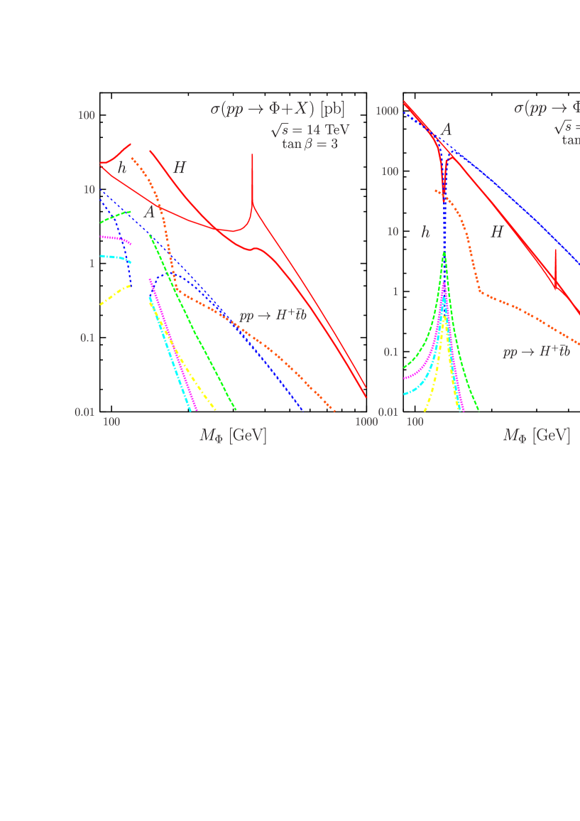
Figure 13: The cross section for the neutral and charged MSSM Higgs production in the main channels at the LHC as a function of their respective masses for $\tan\beta=3$ and $30$ in the maximal mixing scenario; the SM and SUSY inputs are as in Fig. 7.

The principal detection signals of the neutral Higgs bosons at the LHC, in the various regimes of the MSSM, are as follows [37, 38, 35, 36, 19, 53].

In the decoupling regime, i.e. when $M_{h}\simeq M_{h}^{\rm max}$, the lighter $h$ boson is SM–like and has a mass smaller than $\approx 140$ GeV. It can be detected in the $h\to\gamma\gamma$ decays [possibly supplemented with a lepton in associated $Wh$ and $t\bar{t}h$ production], and eventually in $h\to ZZ^{*},WW^{*}$ decays in the upper mass range, and if the vector boson fusion processes are used, also in the decays $h\to\tau^{+}\tau^{-}$ and eventually $h\to WW^{*}$ in the higher mass range $M_{h}\raisebox{-3.69899pt}{~{}\shortstack{$>$ \\ [-0.07cm] $\sim$}}~{}130$ GeV; see Fig. 14 (left). For relatively large values of $\tan\beta$ $(\tan\beta\raisebox{-3.69899pt}{~{}\shortstack{$>$ \\ [-0.07cm] $\sim$}}~{}10)$, the heavier CP–even $H$ boson which has enhanced couplings to down–type fermions, as well as the pseudoscalar Higgs particle, can be observed in the process $pp\to b\bar{b}+H/A$ where at least one $b$–jet is tagged and with the Higgs boson decaying into $\tau^{+}\tau^{-}$, and eventually, $\mu^{+}\mu^{-}$ pairs in the low mass range. With a luminosity of 30 fb^-1 (and in some cases lower) a large part of the $[\tan\beta,M_{A}]$ space can be covered; Fig. 14 (right).

In the anti-decoupling regime, i.e. when $M_{A}<M_{h}^{\rm max}$ and at high $\tan\beta$ ($\raisebox{-3.69899pt}{~{}\shortstack{$>$ \\ [-0.07cm] $\sim$}}~{}10$), it is the heavier $H$ boson which will be SM–like and can be detected as above, while the $h$ boson will behave like the pseudoscalar Higgs particle and can be observed in $pp\to b\bar{b}+h$ with $h\to\tau^{+}\tau^{-}$ or $\mu^{+}\mu^{-}$ provided its mass is not too close to $M_{Z}$ not to be swamped by the background from $Z$ production. The part of the $[\tan\beta,M_{A}]$ space which can be covered is also shown in Fig. 14 (left).

In the intermediate coupling regime, that is for not too large $M_{A}$ values and moderate $\tan\beta\raisebox{-3.69899pt}{~{}\shortstack{$<$ \\ [-0.07cm] $\sim$}}~{}5$, the interesting decays $H\rightarrow hh$, $A\rightarrow hZ$ and even $H/A\rightarrow t\bar{t}$ [as well as the decays $H^{\pm}\to Wh$] still have sizable branching fractions and can be searched for; Fig. 15 (left set). In particular, the $gg\to H\to hh\to b\bar{b}\gamma\gamma$ process (the $4b$ channel is more difficult as a result of the large background) is observable for $\tan\beta\raisebox{-3.69899pt}{~{}\shortstack{$<$ \\ [-0.07cm] $\sim$}}~{}3$ and $M_{A}\raisebox{-3.69899pt}{~{}\shortstack{$<$ \\ [-0.07cm] $\sim$}}~{}300$ GeV, and would allow to measure the trilinear $Hhh$ coupling. These regions of parameter space have to be reconsidered in the light of the new Tevatron value for the top quark mass.

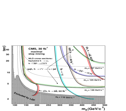
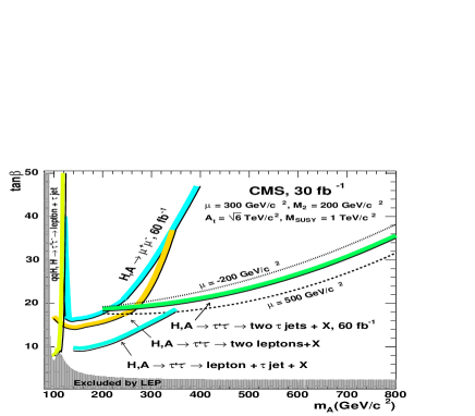
Figure 14: The areas in the $(M_{A},\tan\beta)$ parameter space where the lighter (left) and heavier (right) MSSM neutral Higgs bosons can be discovered at the LHC with an integrated luminosity of 30 fb^-1 in the standard production channels; from [35].

In the intense–coupling regime, that is for $M_{A}\sim M_{h}^{\rm max}$ and $\tan\beta\gg 1$, the three neutral Higgs bosons $\Phi=h,H,A$ have comparable masses and couple strongly to isospin $-\frac{1}{2}$ fermions leading to dominant decays into $b\bar{b}$ and $\tau\tau$ and large total decay widths [52, 53]. The three Higgs bosons can only be produced in the channels $gg\to\Phi$ and $gg/q\bar{q}\to b\bar{b}+\Phi$ with $\Phi\to b\bar{b},\tau^{+}\tau^{-}$ as the interesting $\gamma\gamma,ZZ^{*}$ and $WW^{*}$ decays of the CP–even Higgses are suppressed. Because of background and resolution problems, it is very difficult to resolve between the three particles. A solution advocated in Ref. [53] (see also Ref. [118]), would be the search in the channel $gg/q\bar{q}\to b\bar{b}+\Phi$ with the subsequent decay $\Phi\to\mu^{+}\mu^{-}$ which has a small BR, $\sim 3\times 10^{-4}$, but for which the better muon resolution, $\sim 1\%$, would allow to disentangle between at least two Higgs particles. The backgrounds are much larger for the $gg\to\Phi\to\mu^{+}\mu^{-}$ signals. The simultaneous discovery of the three Higgs particles is very difficult and in many cases impossible, as exemplified in Fig. 15 (right) where one observes only one single peak corresponding to $h$ and $A$ production.

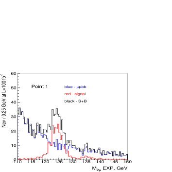
Figure 15: Left: the regions in the $[\tan\beta,M_{A}]$ parameter space where the channel $gg\to H\to hh\to b\bar{b}\gamma\gamma$, $gg\to A\to hZ\to b\bar{b}\ell^{+}\ell^{-}$ and $gg\to H/A\to t\bar{t}\to\ell\nu jjb\bar{b}$ can be detected at the LHC; from Ref. [36]. Right: the $\mu^{+}\mu^{-}$ pair invariant mass distributions for the three Higgs signal peaks with $M_{A}=125$ GeV and $\tan\beta=30$ (leading to $M_{h}\sim 124$ GeV and $M_{H}\sim 134$ GeV) and backgrounds after detector resolution smearing; from Ref. [53].

Finally, as mentioned previously, light $H^{\pm}$ particles with masses below $M_{H^{\pm}}\sim m_{t}$ can be observed in the decays $t\rightarrow H^{+}b$ with $H^{-}\rightarrow\tau\nu_{\tau}$, and heavier ones can be probed for large enough $\tan\beta$, by considering the properly combined $gb\to tH^{-}$ and $gg\rightarrow t\bar{b}H^{-}$ processes using the decay $H^{-}\rightarrow\tau\nu_{\tau}$ and taking advantage of the $\tau$ polarization to suppress the backgrounds, and eventually the decay $H^{-}\to\bar{t}b$ which however, seems more problematic as a result of the large QCD background. See Ref. [119] for more detailed discussions on $H^{\pm}$ production.

4.3 The impact of SUSY particles

The previous discussion on MSSM Higgs production and detection at the LHC might be significantly altered if some supersymmetric particles are relatively light. Some standard production processes can be affected, new processes can occur and the additional detection channels of the Higgs bosons involving SUSY final states might drastically change the detection strategies of the Higgs bosons. Let us briefly comment on some possibilities.

As discussed in section 3.3, the $Hgg$ and $hgg$ vertices in the MSSM are mediated not only by heavy $t/b$ loops but also by loops involving squarks [the NLO QCD corrections are also available [120] and are moderate]. If the top and bottom squarks are relatively light, the cross section for the dominant production mechanism of the lighter $h$ boson in the decoupling regime, $gg\to h$, can be significantly altered by their contributions, similarly to the gluonic decay $h\to gg$. In addition, in the $h\to\gamma\gamma$ decay which is one of the most promising detection channels, the same stop and sbottom loops together with chargino loops, will affect the branching ratio. The cross section times branching ratio $\sigma(gg\rightarrow h)\times{\rm BR}(h\rightarrow\gamma\gamma)$ for the lighter $h$ boson at the LHC can be thus very different from the SM, even in the decoupling limit in which the $h$ boson is supposed to be SM–like [72]. This is illustrated in Fig. 16 (left) where we have simply adopted the low $\tan\beta$ scenario of Fig. 8 for the $h\to gg$ and $\gamma\gamma$ decays. Here again, for light stops and strong mixing which enhances the $h\tilde{t}_{1}\tilde{t}_{1}$ coupling, the effects can be drastic leading to a strong suppression of the cross section $\sigma(gg\rightarrow h\rightarrow\gamma\gamma)$ compared to the SM case.

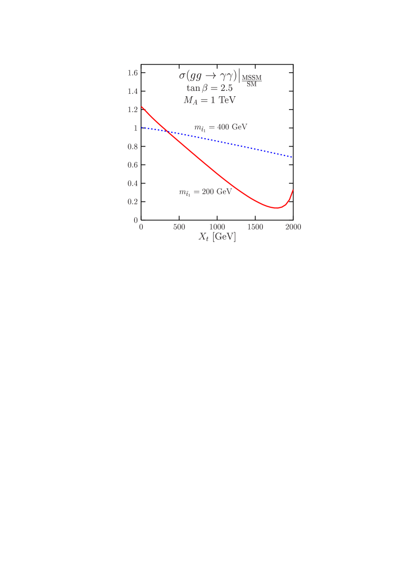
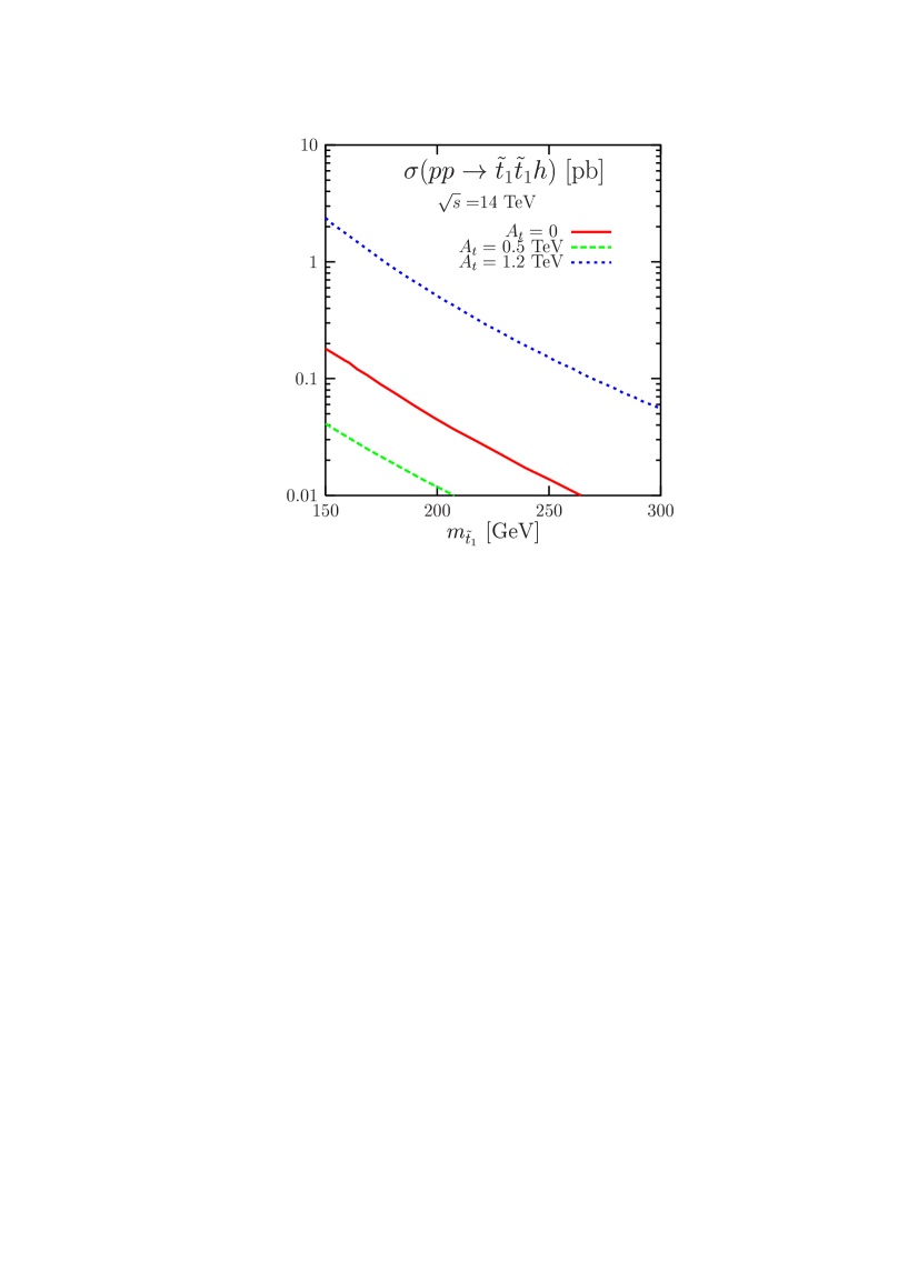
Figure 16: The $gg$–fusion cross section times the photonic branching ratio for the $h$ boson in the MSSM relative to its SM value with stop contributions included [72] (left). The cross section for the process $pp\rightarrow\tilde{t}_{1}\tilde{t}_{1}h$ for threes scenarios of stop mixing [121] (right).

If one of the top squarks is light and its coupling to the $h$ boson is enhanced, an additional process might provide a new source for Higgs particles in the MSSM: associated production with $\tilde{t}_{1}$ states [121], $pp\rightarrow gg/q\bar{q}\rightarrow\tilde{t}_{1}\tilde{t}_{1}h$. This process is similar to the standard $pp\to t\bar{t}h$ mechanism and in fact, for small masses and large mixing of the $\tilde{t}_{1}$ the cross section can be comparable as shown in Fig. 16 (right) where it can reach the picobarn level; in the no or moderate mixing cases, the cross sections are much smaller. The stop will mainly decay into $b\chi_{1}^{+}$, with the chargino decaying into $bW^{+}$ plus missing energy; this leads to $\tilde{t}_{1}\rightarrow bW^{+}$ final states which is the same topology as the decay $t\rightarrow bW^{+}$ except for the larger amount of missing energy which would help isolating the process if the initial production rates are significant. Note that final states with the heavier $H,A,H^{\pm}$ and/or other squark species than $\tilde{t}_{1}$ are less favored by phase space.

Another possible source of MSSM Higgs bosons would be from the cascade decays of strongly interacting sparticles, which have large production rates at the LHC. In particular, the lighter $h$ boson and the heavier $A,H$ and $H^{\pm}$ particles with masses $\raisebox{-3.69899pt}{~{}\shortstack{$<$ \\ [-0.07cm] $\sim$}}~{}200$–300 GeV, can be produced from the decays of squarks and gluinos into the heavier charginos/neutralinos, which then decay into the lighter ones and Higgs bosons. This can occur either in “little cascades”, $\chi_{2}^{0},\chi_{1}^{\pm}\to\chi_{1}^{0}+\,$Higgs, or in “big cascades” $\chi_{3,4}^{0},\chi_{2}^{\pm}\to\chi_{1,2}^{0},\chi_{1}^{\pm}+\,$Higgs. As was shown in Fig. 10, the rates for ino decays into Higgs bosons can be dominant while decays of squarks/gluinos into the heavier inos are substantial. Detailed studies [76, 77] have shown that these processes can be isolated in some areas of the SUSY parameter space. In this case, they can be complementary to the direct production ones in some areas of the MSSM parameter space; see Fig. 17 (left). In particular, one can probe the region $M_{A}\sim 150$ GeV and $\tan\beta\sim 5$, where only $h$ can be observed in standard searches.

One can take advantage of the possibility of light charginos and neutralinos to search for the heavier $H,A$ and $H^{\pm}$ states in regions of the parameter space in which they are not accessible in the standard channels [this is the case e.g. for $M_{A}\sim 200$ GeV and moderate $\tan\beta$ values]. There are situations in which the signals for Higgs decays into charginos and neutralinos are clean enough to be detected at the LHC. One of the possibilities is that the neutral $H/A$ bosons decay into pairs of the second lightest neutralinos, $H/A\to\chi_{2}^{0}\chi_{2}^{0}$, with the subsequent decays of the latter into the LSP neutralinos and leptons, $\chi_{2}^{0}\to\tilde{\ell}^{*}\ell\to\chi_{1}^{0}\ell\ell$ with $\ell^{\pm}=e^{\pm},\mu^{\pm}$, through the exchange of relatively light sleptons. This leads to four charged leptons and missing energy in the final state. If the $H/A$ bosons are produced in the $gg$–fusion processes, there will be little hadronic activity and the $4\ell^{\pm}$ final state is clean enough to be detected. Preliminary analyses show that the decays can be isolated from the large (SUSY) background; Fig. 17 (right). Note that in the scenario in which the Higgs bosons, and in particular the lightest one $h$, decay into invisible lightest neutralinos, the discovery of the particles will be challenging but possible [123].

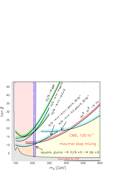
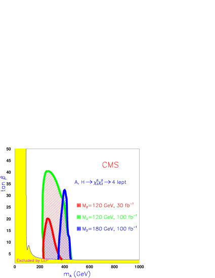
Figure 17: Areas in the $[M_{A},\tan\beta]$ parameter space where the MSSM Higgs bosons can be discovered at the LHC with 100 fb^-1 data in cascades of SUSY particles [77] (left) and in $A/H\rightarrow\chi^{0}_{2}\chi^{0}_{2}\rightarrow 4\ell^{\pm}+X$ decays (right) and for a given set of the MSSM parameters [122].

4.4 Measurements of parameters in the MSSM Higgs sector

In the decoupling regime when the pseudoscalar $A$ boson is very heavy, only the lighter MSSM boson with SM–like properties will be accessible. In this case, the measurements which can be performed for the SM Higgs boson with a mass $\!\raisebox{-3.69899pt}{~{}\shortstack{$<$ \\ [-0.07cm] $\sim$}}~{}\!140$ GeV will also be possible. The $h$ mass can be measured with a very good accuracy, $\Delta M_{h}/M_{h}\!\sim\!0.1\%$, in the $h\!\to\!\gamma\gamma$ decay [35, 36] which incidentally, verifies the spin–zero nature of the particle. However, the total decay width is very small and it cannot be resolved experimentally. The parity quantum numbers will be very challenging to probe [124], in particular since the $h\!\to\!ZZ^{*}\!\to\!4\ell^{\pm}$ decay in which some correlations between the final state leptons can characterize a $J^{\rm PC}\!=\!0^{++}$ particle, might be very rare. This will be also the case of the trilinear Higgs–self coupling which needs extremely high luminosities [125].

Nevertheless, combinations of Higgs production cross sections and decay branching ratios can be measured with a relatively good accuracy [38, 105]. The Higgs couplings to fermions and gauge bosons can be then determined from a fit to all available data. However, while in the SM one could make reasonable theoretical assumptions to improve the accuracy of the measurements, in the MSSM the situation is made more complicated by several features, such as the possibility of invisible decay modes, the radiative corrections in the Higgs sector which can be different for $b,\tau$ and $W/Z$ couplings, $etc.$.. Under some assumptions and with 300 fb^-1 data, one can distinguish an MSSM from a SM Higgs particle at the $3\sigma$ level for $A$ masses up to $M_{A}=$300–400 GeV [105].

The heavier Higgs particles $H,A$ and $H^{\pm}$ are accessible mainly in the $gg\to b\bar{b}+H/A$ and $gb\to H^{\pm}t$ production channels for large $\tan\beta$ values, the main decay modes being $H/A\to b\bar{b},\tau^{+}\tau^{-}$ and $H^{+}\to t\bar{b},\tau^{+}\nu$. The Higgs masses cannot be determined with a very good accuracy as a result of the poor resolution. However, for $M_{A}\raisebox{-3.69899pt}{~{}\shortstack{$<$ \\ [-0.07cm] $\sim$}}~{}300$ GeV and with high luminosities, the $H/A$ masses can be measured with a reasonable accuracy by considering the rare decays $H/A\to\mu^{+}\mu^{-}$ as the resolution on the muon pairs is much better [53, 35]. The discrimination between $H$ and $A$ is nevertheless difficult as the masses are close in general and the total decay widths large [53]. The Higgs spin–parity quantum numbers cannot be probed in these fermionic decays, too.

There is, however, one very important measurement which can be performed in these channels. As the production cross sections above are all proportional to $\tan^{2}\beta$ and, since the ratios of the most important decays fractions are practically independent of $\tan\beta$ for large enough values [when higher–order effects are ignored], one has an almost direct access to this parameter. In Ref. [126], a detailed simulation of the two production channels $gb\to H^{-}t$ and $q\bar{q}/gg\to H/A+b\bar{b}$ at CMS has been performed. At a luminosity of 30 fb^-1 and if only the statistical errors are taken into account, one can make a rather precise measurement, $\Delta\tan\beta/\tan\beta\raisebox{-3.69899pt}{~{}\shortstack{$<$ \\ [-0.07cm] $\sim$}}~{}10\%$ for $M_{A}\raisebox{-3.69899pt}{~{}\shortstack{$<$ \\ [-0.07cm] $\sim$}}~{}400$ GeV. However, there are also systematical errors from e.g. the luminosity measurement and theoretical errors due to the uncertainties on the PDFs [114] and higher–order effects in the production cross sections and decay rates [109, 111]. The theoretical errors are estimated to be $\sim 20\%$ for the production cross section and $\sim 5\%$ for the decay branching ratio. The total accuracy of the measurement worsens then to the level of $\sim 30\%$ for $M_{A}\sim 400$ GeV, $\tan\beta=20$ with 30 fb^-1 data.

Note that in the anti–decoupling regime, it is the heavier CP–even $H$ boson which is SM–like and for which the previously discussed measurements for a SM Higgs particle apply. In this case, the $h$ boson is degenerate in mass with the pseudoscalar Higgs boson and both can be detected in the decays $h/A\to\mu^{+}\mu^{-}$ for large enough values of $\tan\beta$ and $M_{A}\raisebox{-3.69899pt}{~{}\shortstack{$>$ \\ [-0.07cm] $\sim$}}~{}110$ GeV. In the intense–coupling regime, as discussed earlier, the three Higgs bosons will be difficult to disentangle and the situation will be somewhat confusing [53]. In the intermediate–coupling regime, there will be a hope to measure the trilinear $Hhh$ coupling and to have a direct access to part of the scalar potential which breaks the electroweak symmetry. Finally, light SUSY particles would give us the hope to access some important parameters which enter both the Higgs and sparticle sectors.

4.5 The Higgs bosons beyond the CP–conserving MSSM

In the CP–violating MSSM, the production processes of the neutral and charged Higgs particles are the same as in the CP–conserving case once the couplings have been properly adapted. All neutral Higgs particles can be produced in the four dominant processes of Fig. 12. However, in the Higgs–strahlung and vector boson fusion processes, only the CP–even components of the couplings $g_{H_{i}VV}$ will be projected out. The final rates will then simply depend on the masses and couplings of the states $H_{i}$. For the charged Higgs boson, the cross sections are the same as in the CP–conserving MSSM. To illustrate the impact of these CP–violating phases, a benchmark scenario called CPX [63] has been defined using the set of input parameters $\mu=2|A_{t}|=2|A_{b}|=4M_{S}$, while the two basic parameters of the Higgs sector, $\tan\beta$ and $M_{H^{\pm}}$, are allowed to vary. For the CP violating phases, one can assume that the phases of $\mu$ and $M_{3}$ are zero, as these parameters do not play the leading role, while the phases of the trilinear couplings $A_{t}$ and $A_{b}$ are set to a common value $\Phi_{A}$. In this CPX scenario [63], for given $\tan\beta$ and $M_{H^{\pm}}$, there are values of the argument $\Phi_{A}$ for which the mass of the lighter $H_{1}$ boson becomes very small, $M_{H_{1}}\raisebox{-3.69899pt}{~{}\shortstack{$<$ \\ [-0.07cm] $\sim$}}~{}50$ GeV, and at the same time its coupling to the gauge bosons negligible. The other neutral Higgs bosons $H_{2}$ and $H_{3}$ have masses substantially larger than $M_{H_{1}}$ and their couplings to gauge bosons (as well as the trilinear self–couplings) can be substantial as a result of the sum rule $\sum_{i}g_{H_{i}VV}^{2}=g_{H_{\rm SM}VV}^{2}$.

In this scenario, the lighter $H_{1}$ state cannot be observed at the LHC as the cross sections for vector boson fusion $qq\to qqH_{1}$ and Higgs–strahlung $q\bar{q}\to H_{1}V$ are strongly suppressed as a result of the small $g_{H_{1}VV}$ coupling. This is also the case for the production cross section in the gluon–gluon fusion and associated production with top quark pairs: besides the fact that the $ttH_{1}$ coupling is also suppressed, the QCD background events for the dominant $H_{1}\to b\bar{b}$ decays is too large. In turn, since the state $H_{2}$ has couplings that are similar to that of the SM Higgs boson, the rates are substantial in the four production mechanisms and, in particular, in the gluon–gluon $gg\to H_{2}$ and vector boson $qq\to H_{2}qq$ fusion channels. However, the $H_{2}$ state will decay mostly into two $H_{1}$ sates with a branching fraction BR$(H_{2}\to H_{1}H_{1})\raisebox{-3.69899pt}{~{}\shortstack{$>$ \\ [-0.07cm] $\sim$}}~{}80\%$, and the latter will subsequently decay into $b\bar{b}$ pairs with a branching ratio of BR($H_{1}\to b\bar{b})\sim 90\%$. This leads to final state topologies with four $b$ quarks that are subject to a huge QCD background and which will be extremely difficult to detect. Note also that for moderate values of $\tan\beta$, the cross sections for the production of the heavier neutral $H_{3}$ and the charged $H^{\pm}$ Higgs bosons are also too small and no Higgs particle will be thus accessible at the LHC. This is exemplified in the left-hand side of Fig. 18 where the result of an ATLAS simulation show the [$\tan\beta,M_{H^{\pm}}]$ regions of the CP–violating MSSM parameter space that are accessible with 300 fb^-1 data [127].

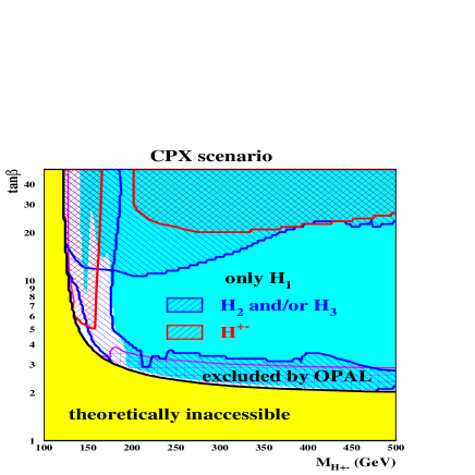
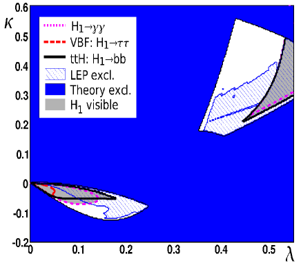
Figure 18: Left: the overall discovery potential for Higgs bosons in ATLAS in a CP–violating scenario after collecting 300 fb^-1 of data, with the white region indicating the area where no Higgs boson can be found; from [127]. Right: regions of the NMSSM parameter space $[\lambda,\kappa$] in which a light pseudoscalar Higgs boson can be detected in an ATLAS simulation [39].

In the NMSSM, where a complex iso-scalar field is introduced, leading to an additional pair of scalar and pseudoscalar Higgs particles, the axion–type or singlino character of the pseudoscalar $A_{1}$ boson makes it preferentially light and decaying into $b$ quarks or $\tau$ leptons [30, 39]. Therefore, in some areas of the NMSSM parameter space, the lightest CP–even Higgs boson may dominantly decay into a pair of light pseudoscalar $A_{1}$ bosons generating four $b$ quarks or $\tau$ leptons in the final state, $H_{1}\to A_{1}A_{1}\to 4b,2b2\tau,4\tau$. In fact, it is also possible that $H_{1}$ is very light with small $VV$ couplings, while $H_{2}$ is not too heavy and plays the role of the SM–like Higgs particle; the decays $H_{2}\to H_{1}H_{1}$ can also be substantial and will give the same signature as above.

This situation, similar to the CPX scenario discussed above, is very challenging at the LHC. Indeed, all the production mechanisms of the light $A_{1}$ or $H_{1}$ singlino–like state will have small cross sections as both couplings to vector bosons and top quarks are tiny. The SM–like Higgs $H_{1}$ or $H_{2}$ will have reasonable production rates but the dominant decay channels into $4b,2\tau 2b$ and $4\tau$ will be swamped by the QCD background. Nevertheless, in the case of very light $A_{1}$ bosons with masses smaller than 10 GeV and, therefore decaying almost exclusively into $\tau^{+}\tau^{-}$ pairs, the $H_{1}\rightarrow A_{1}A_{1}\rightarrow 4\tau\rightarrow 4\mu+4\nu_{\mu}+4\nu_{\tau}$ final state with the $H_{1}$ boson dominantly produced in vector boson fusion can be isolated in some cases. This is exemplified in the right-hand side of Fig. 18 where the result of a simulation of this process by members of the ATLAS collaboration is shown in the parameter space formed by the trilinear NMSSM couplings $\lambda$ and $\kappa$. While there are regions in which the final state can be detected, there are other regions in which the light $H_{1}$ and $A_{1}$states remain invisible even for the high luminosity which has been assumed.

In the most general SUSY model, with an arbitrary number of singlet and doublet fields and an extended matter content to allows for the unification of the gauge couplings, a Higgs boson should have a mass smaller than 200 GeV and significant couplings to gauge bosons and top quarks; this particle can be thus searched for in the $gg$ and $VV$ fusion channels with the signature $WW\to\ell\ell\nu\nu$ which should not be missed. Furthermore, in scenarios with spontaneously broken R–parity, the Higgs particles could decay dominantly into escaping Majorons, $H_{i}\to JJ$ and the searches would also be more complicated than in the usual MSSM. However, invisible decays could be isolated in vector boson fusion or in associated production with a $Z$ boson, albeit with some efforts as the final state is very challenging [123]. In turn, decays of the pseudoscalar Higgs $A_{i}\to H_{j}Z\to Z$ and missing energy could be detected if the cross sections for $A_{i}$ production are large enough.

Other SUSY scenarios can also be probed at the LHC. In GUT theories which lead to the presence of an extra neutral gauge boson at low energies, the $Z^{\prime}$ boson decays $Z^{\prime}\to Zh$ which occur via $Z$–$Z^{\prime}$ mixing could have non–negligible rates and would lead to a detectable $\ell\ell b\bar{b}$ signature [128, 129]; the $Z^{\prime}$ production cross section would be large enough for $M_{Z^{\prime}}\raisebox{-3.69899pt}{~{}\shortstack{$<$ \\ [-0.07cm] $\sim$}}~{}2$ TeV [130] to compensate for the tiny mixing and hence, the small $Z+$Higgs branching ratio. If relatively light doubly charged Higgs bosons exist, they can be produced in the Drell–Yan process $q\bar{q}\to H^{++}H^{--}$ [131] and, if their leptonic decays $H^{--}\to\ell\ell$ are not too suppressed, they would lead to a spectacular 4–lepton final state that cannot be missed.

Hence, many SUSY scenarios beyond the MSSM might lead to an interesting phenomenology which could be probed at the LHC.

5 SUSY Higgs bosons at the ILC

5.1 Higgs production in the SM

In $e^{+}e^{-}$ collisions [40, 41, 42, 43], the main production mechanisms for the SM Higgs particles are the Higgs–strahlung [68, 132] and the $WW$ fusion [82, 133] processes $e^{+}e^{-}\to ZH\to f\bar{f}H$ and $e^{+}e^{-}\to\bar{\nu}_{e}\nu_{e}H$; see Fig. 19 (left). The final state $H\nu\bar{\nu}$ is generated in both the fusion and Higgs–strahlung processes. Besides the $ZZ$ fusion mechanism [82, 133] $e^{+}e^{-}\to e^{+}e^{-}H$ which is similar to $WW$ fusion but with an order of magnitude smaller cross section, sub–leading Higgs production channels are associated production with top quarks $e^{+}e^{-}\to t\bar{t}H$ [134] and double Higgs production [135, 136] in the Higgs–strahlung $e^{+}e^{-}\to ZHH$ and fusion $e^{+}e^{-}\to\bar{\nu}\nu HH$ processes. Despite the smaller production rates, the latter mechanisms are very useful when it comes to the study of the Higgs fundamental properties. The production rates for all these processes are shown in Fig. 19 (center) at a c.m. energy of $\sqrt{s}\!=\!500$ GeV as a function of $M_{H}$.

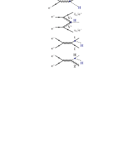
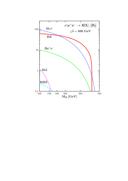
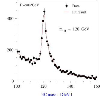
Figure 19: Production mechanisms (left), the total cross sections as a function of $M_{H}$ [18] (center) and the detection for $M_{H}=120$ GeV [41] (right) of the SM Higgs boson at the ILC.

The cross section for Higgs–strahlung scales as $1/s$ and therefore dominates at low energies, while the one of the $WW$ fusion mechanism rises like $\log(s/M_{H}^{2})$ and becomes more important at high energies. The electroweak radiative corrections to both processes are known and are under control [137, 138]. At $\sqrt{s}\sim 500$ GeV, the two processes have approximately the same cross sections, ${\cal O}(50~{}{\rm fb})$ for the interesting Higgs mass range 115 GeV$\,\raisebox{-3.69899pt}{~{}\shortstack{$<$ \\ [-0.07cm] $\sim$}}~{}M_{H}\raisebox{-3.69899pt}{~{}\shortstack{$<$ \\ [-0.07cm] $\sim$}}~{}\,$200 GeV favored by high–precision data. For the expected ILC integrated luminosity ${\cal L}\sim 500$ fb^-1, about 35000 events can be collected in the $e^{+}e^{-}\to HZ$ and $e^{+}e^{-}\to\nu\bar{\nu}H$ channels for $M_{H}\sim 120$ GeV, which is more than enough to observe the Higgs particle and to study its properties in great detail.

Turning to the sub–leading processes, the $ZZ$ fusion mechanism $e^{+}e^{-}\to He^{+}e^{-}$ is similar to $WW$ fusion but has a cross section that is one order of magnitude smaller; however, the full final state can be reconstructed. The associated production with top quarks has a very small cross section at $\sqrt{s}=500$ GeV due to phase space suppression but, at $\sqrt{s}=800$ GeV, it can reach the level of a few fbs. The $t\bar{t}H$ final state is generated almost exclusively through radiation off top quarks, thus allowing an unambiguous determination of the $g_{Htt}$ Yukawa coupling; the process is also very sensitive to the spin–parity of the $H$ boson [140]. The electroweak and QCD corrections are moderate [141], except near threshold where large coulombic corrections occur and double the production rate. For $M_{H}\raisebox{-3.69899pt}{~{}\shortstack{$<$ \\ [-0.07cm] $\sim$}}~{}140$ GeV, the main signal $t\bar{t}H\to W^{+}W^{-}b\bar{b}b\bar{b}$ is spectacular and $b$–tagging as well as the reconstruction of the $M_{H}$ peak are essential to suppress the large backgrounds. For $M_{H}\raisebox{-3.69899pt}{~{}\shortstack{$>$ \\ [-0.07cm] $\sim$}}~{}140$ GeV, the process leads mainly to $Ht\bar{t}\to 4Wb\bar{b}$ final states which give rise to ten jets if all $W$ bosons are allowed to decay hadronically to increase the statistics.

The cross section for double Higgs production in the strahlung process, $e^{+}e^{-}\to HHZ$, is at the level of $\sim\frac{1}{2}$ fb at $\sqrt{s}=500$ GeV for a light Higgs boson, $M_{H}\sim 120$ GeV, and is smaller at higher energies [136]. It is rather sensitive to the trilinear Higgs–self coupling $\lambda_{HHH}$: for $\sqrt{s}\!=\!500$ GeV and $M_{H}\!=\!120$ GeV for instance, it varies by about 20% for a 50% variation of $\lambda_{HHH}$. The electroweak corrections to the process have been shown to be moderate [142]. The characteristic signal for $M_{H}\raisebox{-3.69899pt}{~{}\shortstack{$<$ \\ [-0.07cm] $\sim$}}~{}140$ GeV consists of four $b$–quarks to be tagged and a $Z$ boson which needs to be reconstructed in both leptonic and hadronic final states to increase the statistics. For higher Higgs masses, the dominant signature is $Z+4W$ leading to multi–jet (up to 10) and/or multi–lepton final states. The rate for double Higgs production in $WW$ fusion, $e^{+}e^{-}\to\nu_{e}\bar{\nu}_{e}HH$, is extremely small at $\sqrt{s}=500$ GeV but increases with energy to reach the level of $\frac{1}{2}$ fb at 1 TeV.

Finally, future linear colliders can be turned to $\gamma\gamma$ colliders, in which the photon beams are generated by Compton back–scattering of laser light with c.m. energies and integrated luminosities only slightly lower than that of the original $e^{+}e^{-}$ collider. Tuning the maximum of the $\gamma\gamma$ spectrum to the value of $M_{H}$, the Higgs can be formed as $s$–channel resonances, $\gamma\gamma\to H$, decaying mostly into $b\bar{b}$ and/or $WW^{*},ZZ^{*}$ final states. This allows precise measurement of the Higgs couplings to photons as well as the CP nature of the Higgs particle [139]. The $e^{-}e^{-}$ option is also possible.

In Higgs–strahlung, the recoiling $Z$ boson is mono–energetic and the Higgs mass can be derived from the $Z$ energy when the initial $e^{\pm}$ beam energies are sharp (the effects of beamstrahlung must be thus suppressed as strongly as possible). The $Z$ boson can be tagged through its clean $\ell^{+}\ell^{-}$ decays ($\ell\!=\!e,\mu$) but also through decays into quarks which have a much larger statistics. Therefore, it will be easy to separate the signal from the backgrounds. In the low mass range, $M_{H}\!\raisebox{-3.69899pt}{~{}\shortstack{$<$ \\ [-0.07cm] $\sim$}}~{}\!140$ GeV, the process leads to $b\bar{b}q\bar{q}$ and $b\bar{b}\ell\ell$ final states, with the $b$ quarks being efficiently tagged by micro–vertex detectors. For $M_{H}\!\raisebox{-3.69899pt}{~{}\shortstack{$>$ \\ [-0.07cm] $\sim$}}~{}\!140$ GeV where the decay $H\to WW^{*}$ dominates, the Higgs boson can be reconstructed by looking at the $\ell\ell+\,$4–jet or 6–jet final states, and using the kinematical constraints on the fermion invariant masses which peak at $M_{W}$ and $M_{H}$, the backgrounds are efficiently suppressed. Also the $\ell\ell q\bar{q}\ell\nu$ and $q\bar{q}q\bar{q}\ell\nu$ channels are easily accessible.

It has been shown in detailed simulations [41, 42] that only a few fb^-1 data are needed to obtain a 5$\sigma$ signal for a Higgs boson with a mass $M_{H}\sim 120$ GeV at a 350 GeV collider; see Fig. 19 (right) with 500 fb^-1 data. In fact, for such small masses, it is better to move to lower energies where the Higgs–strahlung cross section is larger and the reconstruction of the $Z$ boson is better [143]. Moving to higher energies, Higgs bosons with masses up to $M_{H}\sim 400$ GeV can be discovered in the Higgs–strahlung process at an energy of 500 GeV and with a luminosity of 500 fb^-1. For even larger masses, one needs to increase the c.m. energy of the collider and, as a rule of thumb, Higgs masses up to $\sim 80$% $\sqrt{s}$ can be probed. This means that a 1 TeV collider can probe the entire Higgs mass range that is theoretically allowed in the SM, $M_{H}\raisebox{-3.69899pt}{~{}\shortstack{$<$ \\ [-0.07cm] $\sim$}}~{}700$ GeV.

The $WW$ fusion mechanism offers a complementary production channel. For low $M_{H}$ where the decay $H\to b\bar{b}$ is dominant, flavor tagging plays an important role to suppress the background. The $e^{+}e^{-}\to H\bar{\nu}\nu\to b\bar{b}\bar{\nu}\nu$ final state can be separated from the corresponding one in the process, $e^{+}e^{-}\to HZ\to b\bar{b}\bar{\nu}\nu$, by exploiting their different characteristics in the $\nu\bar{\nu}$ invariant mass [41]. The polarization of the $e^{\pm}$ beams, which allows tuning of the $WW$ fusion contribution, can be very useful to control the systematic uncertainties. For larger $M_{H}$, when the decays $H\to WW^{(*)},ZZ^{(*)}$ and even $t\bar{t}$ are dominant, the backgrounds can be suppressed using kinematical constraints from the reconstruction of the Higgs mass peak and exploiting the signal characteristics.

5.2 Higgs production in the MSSM

At the ILC, besides the usual Higgs–strahlung and fusion processes for $h$ and $H$ production, the neutral Higgs particles can also be produced pairwise: $e^{+}e^{-}\to A+h/H$ [144]. The cross sections for the Higgs–strahlung and the pair production as well as the cross sections for the production of $h$ and $H$ are mutually complementary, coming either with a coefficient $\sin^{2}(\beta-\alpha)$ or $\cos^{2}(\beta-\alpha)$; Fig. 20. The cross section for $hZ$ production is large for large values of $M_{h}$, being of ${\cal O}(100$ fb) at $\sqrt{s}=500$ GeV; by contrast, the cross section for $HZ$ is large for light $h$ (implying small $M_{H}$). In major parts of the parameter space, the signals consist of a $Z$ boson and $b\bar{b}$ or $\tau^{+}\tau^{-}$ pairs, which is easy to separate from the backgrounds with flavor tagging. For associated production, the situation is opposite: the cross section for $Ah$ is large for light $h$ whereas $AH$ production is preferred in the complementary region. The signals consists mostly of four final $b$ quarks, requiring efficient $b$–quark tagging; mass constraints help to eliminate the QCD jets and $ZZ$ backgrounds. The CP–even Higgs particles can also be searched for in the $WW$ and $ZZ$ fusion mechanisms.

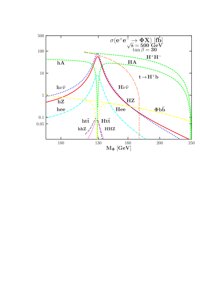
Figure 20: Production cross sections of the MSSM Higgs bosons in $e^{+}e^{-}$ collisions as functions of the masses for $\tan\beta=30$ and $\sqrt{s}=500$ GeV; from Ref. [19].

In $e^{+}e^{-}$ collisions, charged Higgs bosons can be produced pairwise, $e^{+}e^{-}\to H^{+}H^{-}$, through $\gamma,Z$ exchange. The cross section depends only on the charged Higgs mass; it is large almost up to $M_{H^{\pm}}\sim\frac{1}{2}\sqrt{s}$. $H^{\pm}$ bosons can also be produced in top decays; in the range $1<\tan\beta<m_{t}/m_{b}$, the $t\to H^{+}b$ branching ratio and the $t\bar{t}$ production cross sections are large enough to allow for their detection in this mode. [$H^{\pm}$ can also be pair–produced in $\gamma\gamma$ collisions with large rates].

The discussion of SUSY Higgs production at ILC can be summarized in the following points.

– The Higgs boson $h$ can be detected in the entire range of the MSSM parameter space, either through the Higgs–strahlung (and $WW$ fusion) process or associated production with the pseudoscalar $A$ boson. In fact, this conclusion holds true even at a c.m. energy of 250 GeV and with a luminosity of a few fb^-1. Even if the decay modes of the $h$ boson are very complicated, missing mass techniques allow for their detection. For instance, the branching ratios for the invisible $h$ boson decays into the LSP neutralinos can be measured at the percent level; see Fig. 21 (left). The accuracy can be substantially improved by running at lower c.m. energies [143]. The same very detailed tests and precision measurements for the SM Higgs boson (see later) can be performed for the MSSM $h$ boson, in particular in the decoupling limit, thus complementing LHC analyses [40].

– All SUSY Higgs bosons can be discovered at an $e^{+}e^{-}$ collider if the $H,A$ and $H^{\pm}$ masses are less than the beam energy; for higher masses, one simply has to increase the c.m. energy, $\sqrt{s}\raisebox{-3.69899pt}{~{}\shortstack{$>$ \\ [-0.07cm] $\sim$}}~{}2M_{A}$. Several channels might be observable depending on the value of $\tan{\beta}$. The dominant processes will be however Higgs pair production $e^{+}e^{-}\to HA$ and $H^{+}H^{-}$ for which the cross sections are not suppressed by mixing factors (for $M_{A}\raisebox{-3.69899pt}{~{}\shortstack{$>$ \\ [-0.07cm] $\sim$}}~{}M_{h}^{\rm max}$ in the case of $HA$ production). This is exemplified in the central and right–handed panels of Fig. 21. Note that the additional associated neutral Higgs production processes with $t\bar{t}$ and $b\bar{b}$ allow for the measurement of the Yukawa couplings. In particular, $e^{+}e^{-}\to b\bar{b}+h/H/A$ for high $\tan\beta$ values allow for the determination of the important $\tan\beta$ parameter for low $M_{A}$ values.

– If the energy is not high enough to open the $HA$ pair production threshold, the photon collider option may become the discovery machine for the heavy Higgs bosons [139, 145]. Since the $A,H$ bosons are produced as $s$–channel resonances, the mass reach at a photon collider is extended compared to the $e^{+}e^{-}$ mode and masses up to 80% of the original c.m. energy can be probed. It has been shown in Ref. [145] that the whole medium $\tan{\beta}$ region up to about 500 GeV, where only one light Higgs boson can be found at the LHC (the so–called wedge region of the LHC), can be covered by the photon collider option with three years of operation with an $e^{-}e^{-}$ c.m. energy of 630 GeV. The photon collider mode is also important to determine the CP properties of the heavy Higgs bosons, either by studying angular correlation of Higgs decay products or by using initial beam polarization. The discrimination between the scalar and pseudoscalar particles can be performed and CP violation can be unambiguously probed [146] .

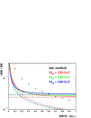
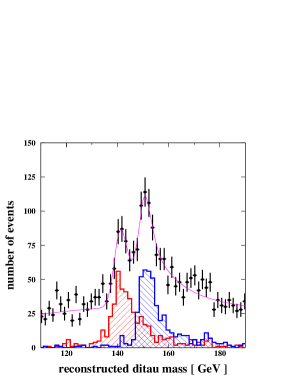
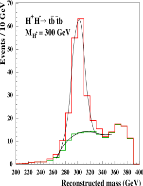
Figure 21: The expected accuracy on the invisible decay rate as a function of the branching ratio at $\sqrt{s}=350$ GeV in full lines; the other lines are from measurement of the invisible rate (dashed), the total cross section (dotted) and an indirect method (large dots) [147] (left). The reconstructed $\tau\tau$ invariant mass from a kinematic fit in $e^{+}e^{-}\!\to\!HA\!\to\!b\bar{b}\tau^{+}\tau^{-}$ for $M_{A}\!=\!140$ GeV and $M_{H}\!=\!150$ GeV at $\sqrt{s}\!=\!500$ GeV [148] (center). The di–jet invariant mass distribution for the $e^{+}e^{-}\!\to\!H^{+}H^{-}\!\to\!t\bar{b}\bar{t}b$ process for $M_{H^{\pm}}\!=\!300$ GeV after final state constraints at $\sqrt{s}\!=\!800$ GeV [41] (right). In all cases, a luminosity of 500 fb^-1 is assumed.

5.3 High–precision measurements of the Higgs properties

The profile of the lighter Higgs boson can be entirely determined. This is particularly the case close to the decoupling regime where the $h$ boson behaves like the SM Higgs particle but with a mass below $M_{h}\sim 140$ GeV. This is, in fact, the most favorable mass range for precision measurements as the Higgs boson has many decay channels that are accessible in this case. A short summary of the measurements which can be performed is as follows; see Refs. [41, 42, 43] for details and references.

$\bullet$ The measurement of the recoil $f\bar{f}$ mass in the Higgs–strahlung process, $e^{+}e^{-}\rightarrow hf\bar{f}$ allows a very good determination of the Higgs mass: at $\sqrt{s}=350$ GeV and with $500$ fb^-1 data, a precision of $\Delta M_{h}\sim 50$ MeV can be reached for $M_{h}\sim 120$ GeV. [Accuracies $\Delta M_{H}\sim 80$ MeV can also be reached for $M_{H}=150$ and 180 GeV when the heavier Higgs decays mostly into gauge bosons.]

$\bullet$ The angular distribution of the $Z/h$ in the strahlung process, $\sim\sin^{2}\theta$ at high energy, characterizes the production of a $J^{P}=0^{+}$ particle. The Higgs spin–parity quantum numbers can also be checked by looking at correlations in the production $e^{+}e^{-}\rightarrow hZ\rightarrow 4f$ or decay $h\rightarrow WW^{*}\rightarrow 4f$ processes, as well as in the channel $h\rightarrow\tau^{+}\tau^{-}$. An unambiguous test of the CP nature of the $h$ boson can be made in threshold and polarization analyses in the process $e^{+}e^{-}\rightarrow t\bar{t}h$ [or at laser photon colliders in the loop–induced process $\gamma\gamma\rightarrow h$].

$\bullet$ The Higgs couplings to $ZZ/WW$ bosons, which are predicted to be proportional to the masses, can be directly determined by measuring the production cross sections in the strahlung and the fusion processes. In the $e^{+}e^{-}\rightarrow\ell^{+}\ell^{-}+h$ and $\nu\bar{\nu}+h$ processes, the total cross section can be measured with a precision less than $\sim$ 3% at $\sqrt{s}\sim 500$ GeV with 500 fb^-1 integrated luminosity if $h$ is SM–like. This leads to an accuracy of less than 1.5% on the $hVV$ couplings.

$\bullet$ The measurement of the Higgs branching ratios is of utmost importance. Since $M_{h}\raisebox{-3.69899pt}{~{}\shortstack{$<$ \\ [-0.07cm] $\sim$}}~{}130$ GeV, a large variety of branching ratios can be measured: the $b\bar{b},c\bar{c}$ and $\tau^{+}\tau^{-}$ branching ratios allow us to derive the relative Higgs–fermion couplings and to check the prediction that they are proportional to the masses. The gluonic branching ratio is sensitive to the $t\bar{t}h$ Yukawa coupling and to new strongly interacting particles, such as stops in the MSSM. The branching ratio into $W$ bosons allows a measurement of the $hWW$ coupling, while the branching ratio of the loop–induced $\gamma\gamma$ decay is also very important since it is sensitive to new particles.

$\bullet$ The Higgs coupling to top quarks, which is the largest coupling in the theory, is directly accessible in the process where the Higgs boson is radiated off top quarks, $e^{+}e^{-}\rightarrow t\bar{t}h$. For $M_{h}\raisebox{-3.69899pt}{~{}\shortstack{$<$ \\ [-0.07cm] $\sim$}}~{}130$ GeV, the Yukawa coupling can be measured with a precision of less than 5% at $\sqrt{s}\sim 800$ GeV with a luminosity of ${\cal L}\sim 1$ ab^-1.

$\bullet$ The total width of the SM Higgs boson, for masses less than $\sim 200$ GeV, is so small that it cannot be resolved experimentally. However, the measurement of BR($h\rightarrow WW$) allows an indirect determination of $\Gamma_{h}$, since the $hWW$ coupling can be determined from the measurement of the Higgs cross section in the $WW$ fusion process. [$\Gamma_{\rm tot}$ can also be derived by measuring the $\gamma\gamma\to h$ cross section at a $\gamma\gamma$ collider or the branching ratio of $h\to\gamma\gamma$ in $e^{+}e^{-}$ collisions].

$\bullet$ Finally, the measurement of the trilinear Higgs self–coupling, which is the first non–trivial test of the Higgs potential, is accessible in the double Higgs production processes $e^{+}e^{-}\rightarrow Zhh$ [and in the $e^{+}e^{-}\rightarrow\nu\bar{\nu}hh$ process at high energies]. Despite its smallness, the cross sections can be determined with an accuracy of the order of 20% at a 500 GeV collider if a high luminosity, ${\cal L}\sim 1$ ab^-1, is available. [For not too large $M_{H}$, the coupling $\lambda_{Hhh}$ can also be accessed.]

An illustration of the experimental accuracies that can be achieved in the determination of the mass, CP–nature, total decay width and the various couplings of a SM–like Higgs boson for the two masses $M_{h}=120$ and 140 GeV is shown in Table 1 for $\sqrt{s}=350$ GeV [for $M_{h}$ and the CP nature] and $500$ GeV [for $\Gamma_{\rm tot}$ and all couplings except for $g_{htt}$] and for $\int{\cal L}=500$ fb^-1 [except for $g_{htt}$ where $\sqrt{s}=1$ TeV and $\int{\cal L}=1$ ab^-1 are assumed]. The achievable accuracy is impressive.

$M_{h}$ (GeV)	$\Delta M_{h}$	$\Delta{\rm CP}$	$\ \Gamma_{\rm tot}\$	$g_{hWW}$	$g_{hZZ}$	$g_{htt}$	$g_{hbb}$	$g_{hcc}$	$g_{h\tau\tau}$	$g_{hhh}$
$120$	$\pm 0.033$	$\pm 3.8$	$\pm 6.1$	$\pm 1.2$	$\pm 1.2$	$\pm 3.0$	$\pm 2.2$	$\pm 3.7$	$\pm 3.3$	$\pm 17$
$140$	$\pm 0.05$	$-$	$\pm 4.5$	$\pm 2.0$	$\pm 1.3$	$\pm 6.1$	$\pm 2.2$	$\pm 10$	$\pm 4.8$	$\pm 23$

Table 1: Relative accuracies (in %) on the SM–like Higgs boson mass, width and couplings obtained at the ILC with $\sqrt{s}=350,500$ GeV and $\int{\cal L}=500$ fb^-1 (except for top); Ref. [41].

A number of very important measurements can be performed at the ILC in the MSSM heavier Higgs sector. If the $H,A$ and $H^{\pm}$ states are kinematically accessible, one can measure their masses and cross sections times decay branching ratios with a relatively good accuracy. In the pair production process $e^{+}e^{-}\to HA$, a precision of the order of $0.2\%$ can be achieved on the $H$ and $A$ masses, while a measurement of the cross sections can be made at the level of a few percent in the $b\bar{b}b\bar{b}$ and ten percent in the $b\bar{b}\tau^{+}\tau^{-}$ channels. For the charged Higgs boson, statistical uncertainties of less than 1 GeV on its mass and less than 15% on its production cross section times branching ratio can be achieved in the channel $e^{+}e^{-}\to H^{+}H^{-}\to t\bar{b}\bar{t}b$ for $M_{H^{\pm}}\sim 300$ GeV with high enough energy and luminosity.

These measurements allow the determination of the most important branching ratios, $b\bar{b}$ and $\tau^{+}\tau^{-}$ for the $H/A$ and $tb$ and $\tau\nu$ for the $H^{\pm}$ particles, as well as the total decay widths which can be turned into a determination of the value of $\tan\beta$, with an accuracy of 10% or less. The spin–zero nature of the particles can be easily checked by looking at the angular distributions which should go as $\sin^{2}\theta$. Several other measurements, such as the spin–parity of the Higgs particles in $H/A\to\tau^{+}\tau^{-}$ decays and, in favorable regions of the parameter space, some trilinear Higgs couplings such as $\lambda_{Hhh}$, can be made.

The high–precision achievable at the ILC in the SUSY Higgs sector would allow to determine two very important parameters, $\tan\beta$ and $M_{A}$, which can be used as inputs in the extrapolation of low energy scenarios to the GUT scale to reconstruct the fundamental SUSY theory.

5.4 Global analyses and LHC–ILC complementarity

A detailed analysis of the deviations of the couplings of the $h$ boson with a mass $M_{h}=120$ GeV, from the predictions in the SM has been performed in Ref. [41] using a complete scan of the MSSM $[M_{A},\tan\beta]$ parameter space, including radiative corrections. In Fig. 22, shown are the 1$\sigma$ and 95% confidence level contours for the fitted values of various pairs of ratios of couplings, assuming the experimental accuracies at the ILC discussed in the previous section and summarized in Tab. 1.

From a $\chi^{2}$ test which compares the deviations, the MSSM can be distinguished from the SM case at the 95% confidence level for $M_{A}\raisebox{-3.69899pt}{~{}\shortstack{$<$ \\ [-0.07cm] $\sim$}}~{}600$ GeV (and only at the 68% confidence level for $M_{A}\raisebox{-3.69899pt}{~{}\shortstack{$<$ \\ [-0.07cm] $\sim$}}~{}750$ GeV). In some cases, one is sensitive to MSSM effects even for masses $M_{A}\!\sim\!1\;$TeV, i.e. beyond the LHC mass reach. If the deviations compared to the SM are large, these precision measurements would also allow for an indirect determination of $M_{A}$; for instance, in the mass range $M_{A}=300$–600 GeV an accuracy of 70–100 GeV is possible on the $A$ mass.

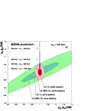
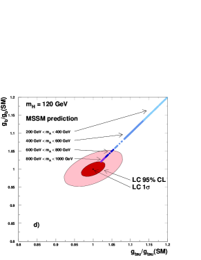
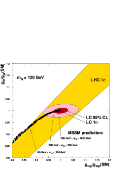
Figure 22: Determination of the couplings of a SM–like Higgs boson at the ILC and the interpretation within the MSSM. The contours are the couplings of a 120 GeV Higgs boson as measured with 500 fb^-1 data at $\sqrt{s}=350$ GeV except for $g_{Htt}$ which uses 800 GeV (here the expectation at the LHC is also shown); from Ref. [41].

This type of indirect determination cannot be made in a convincing way at the LHC as the experimental errors in the various measurements are worse than at the ILC; see Fig. 22 (right) where the $g_{hWW}$ and $g_{htt}$ contours are displayed. While at the ILC, MSSM effects can be probed for masses close to $M_{A}=1$ TeV, there is practically no sensitivity at the LHC. However, the precision measurements at the ILC can gain enormously from other measurements that can be performed only at the LHC.

Indeed, the various Higgs couplings are not only sensitive to the tree–level inputs $M_{A}$ and $\tan\beta$ but also, on parameters that enter through radiative corrections such as the stop and sbottom masses which could be accessible only at the LHC. If, in addition, the $A$ boson is seen at the LHC (which means that $\tan\beta$ is large, $\tan\beta\raisebox{-3.69899pt}{~{}\shortstack{$>$ \\ [-0.07cm] $\sim$}}~{}10$) and its mass is measured at the level of 10%, the only other important parameter entering the Higgs sector at one–loop is the trilinear coupling $A_{t}$ (and to a lesser extent, $A_{b}$ and $\mu$) which will be only loosely constrained at the LHC. Nevertheless, using this knowledge and the fact that the top mass (the uncertainty of which generates the largest error as the corrections are $\propto m_{t}^{4}$) can be measured with a precision of 100 MeV at the ILC, one can vastly improve the tests of the MSSM Higgs sector that can be performed at the LHC or at the ILC alone. This is one example of the possible complementarity between the LHC and the ILC; for more discussions and examples see Ref. [40].

5.5 Extended Higgs sectors at the ILC

In the CP–violating MSSM where the three neutral Higgs bosons $H_{1},H_{2},H_{3}$ are mixtures of CP–even and CP–odd states, because of the sum rule for the Higgs couplings to gauge bosons, $\sum_{i}g_{H_{i}VV}^{2}=g^{2}_{H_{SM}}$, the production cross sections in the Higgs–strahlung and $WW$ fusion processes should be large for at least one of the particles and there is a complementarity between $H_{i}$ single and $H_{j}H_{k}$ pair production. In fact, similarly to the usual MSSM, the normalized couplings are such that $|g_{H_{1}VV}|=|g_{H_{2}H_{3}V}|\sim 1$ in the decoupling limit $M_{H^{\pm}}\raisebox{-3.69899pt}{~{}\shortstack{$>$ \\ [-0.07cm] $\sim$}}~{}200$ GeV and at least $H_{1}$ is accessible for $\sqrt{s}\raisebox{-3.69899pt}{~{}\shortstack{$>$ \\ [-0.07cm] $\sim$}}~{}300$ GeV, since $M_{H_{1}}\raisebox{-3.69899pt}{~{}\shortstack{$<$ \\ [-0.07cm] $\sim$}}~{}130$ GeV. If two or the three Higgs particles are very close in mass, the excellent energy and momentum resolution on the recoiling $Z$ boson in the Higgs–strahlung process would allow to resolve the coupled Higgs systems, e.g. from an analysis of the lineshape (this is in fact similar to the MSSM in the intense coupling regime). . The presence of CP–violation can be unambiguously checked by studying the spin–spin correlations in Higgs decays into tau lepton pairs or controlling the beam polarization of the colliding photon beams at the $\gamma\gamma$ option of the ILC; see Ref. [146] for instance.

The ILC will also be very useful in probing the Higgs sector of the NMSSM with the additional CP–even and CP–odd Higgs particles. As seen previously, Higgs–strahlung, $e^{+}e^{-}\to ZH_{i}$, allows for the detection of CP–even Higgs particles independently of their decay modes and thus, even if they decay into the singlino–like light $A_{1}$ or $H_{1}$ states. This is possible provided that their couplings to the $Z$ boson are substantial, as it always occurs for at least one CP–even Higgs boson. In fact, thanks to the usual sum rule which relates the CP–even Higgs couplings to the those of the SM Higgs boson, a “no–lose theorem” for discovering at least one Higgs state has been established for ILC while for LHC, as discussed in the previous subsection, the situation is presently less clear and all Higgs particles could escape detection.

In the general SUSY scenario with an arbitrary number of singlet and doublet fields, one Higgs particle has significant $ZZ$ coupling and a mass smaller than 200 GeV. This particle should be therefore kinematically accessible at the ILC with a c.m. energy $\sqrt{s}\raisebox{-3.69899pt}{~{}\shortstack{$>$ \\ [-0.07cm] $\sim$}}~{}350$ GeV. It can be detected in the Higgs–strahlung process independently of its (visible or invisible) decay modes. If its mass happens to be in the high range, $M_{h}\sim 200$ GeV, at least its couplings to $W,Z$ bosons and $b$–quarks (eventually $t$–quarks at high energies and luminosities), as well as the total decay widths and the spin–parity quantum numbers can be determined.

We should stress again that even in scenarios with invisible Higgs decays, as would be the case for instance of spontaneously broken R–parity scenarios in which the Higgs particles could decay dominantly into invisible Majorons, $H_{i}\to JJ$, at least one CP–even Higgs boson is light and has sizable couplings to the gauge bosons and should be observed by studying the recoil mass spectrum against the $Z$ boson in the Higgs–strahlung process. Furthermore, if doubly charged Higgs bosons of left–right symmetric models occur [32, 33] and if kinematically accessible at the ILC, they can be pair produced in $e^{+}e^{-}$ collisions, $e^{+}e^{-}\to H^{++}H^{--}$ with large rates [also in $\gamma\gamma$ collisions where, because of the large electric charge, the rates are more than an order of magnitude larger than for singly charged $H^{\pm}$ bosons]; they can also be singly produced in $e^{-}e^{-}$ collisions, and thus with a much more favorable phase space, if the Yukawa couplings are not too small [149]. Finally, in the presence of a new $Z^{\prime}$ boson [128, 150], the Higgs–strahlung process would receive additional contributions from the virtual exchange of this new particle, $e^{+}e^{-}\to Z,Z^{\prime}\to hZ$, and thanks to the high–luminosity and to the clean environment, the expectedly small deviations of the production cross section from the SM or MSSM cases could be detected.

Thus, from the previous discussions, one can thus conclude that the ILC is an ideal machine for the SUSY Higgs sector, whatever scenario nature has chosen.

6 Conclusion

The LHC will soon provide us with the answer to the question that particle physicists are asking themselves since the seminal paper of Julius Wess and Bruno Zumino, almost four decades ago: is low–energy Supersymmetry realized in Nature? The answer might first come from the Higgs sector, as a generic prediction of low–energy SUSY is the existence of at least one light Higgs particle with a mass below $\sim 200$ GeV. If the answer to the question is positive, a new continent will be open to experimental investigation as well as theoretical development. While the LHC will make the pioneering exploration of the new continent, the ILC will be needed to fully chart it.

We are anxiously waiting for these breathtaking times. Much to our regret, Julius Wess will not be among us during these times.

Acknowledgments: I thank J. Bartels and S. Bethke for inviting me to write this review and for their patience while waiting for the manuscript and P.M. Zerwas for comments on the draft. Support from the Alexander von–Humbold Foundation (Bonn, Germany) is acknowledged.

Appendix

In this appendix we sketch the derivation of the scalar Higgs potential eq. (2) from the SUSY Superpotential and its soft–SUSY breaking counterpart.

The most general globally supersymmetric superpotential, compatible with gauge invariance, renormalizability and $R$–parity conservation can be written in terms of (hatted) superfields, as

$${\cal W}=\sum_{i,j=\rm generation}-Y^{u}_{ij}\,{\widehat{u}}_{Ri}\widehat{H_{2}}\!\cdot\!{\widehat{Q}}_{j}+Y^{d}_{ij}\,{\widehat{d}}_{Ri}\widehat{H}_{1}\!\cdot\!{\widehat{Q}}_{j}+Y^{\ell}_{ij}\,{\widehat{\ell}}_{Ri}\widehat{H}_{1}\!\cdot\!{\widehat{L}}_{j}+\mu\widehat{H}_{2}\!\cdot\!\widehat{H}_{1}$$

The product between SU(2)_L doublets for Higgses, quarks and leptons reads $H\cdot Q\equiv\epsilon_{ab}H^{a}Q^{b}$; etc… where $a,b$ are SU(2)_L indices and $\epsilon_{12}=1=-\epsilon_{21}$; $Y^{u,d,\ell}_{ij}$ denote the Yukawa couplings among generations. The first three terms are nothing else but a superspace generalization of the Yukawa interaction in the SM, while the last term is a globally supersymmetric Higgs mass term.

The supersymmetric part of the tree–level scalar potential is the sum of the F– and D–terms, where the F–terms come from the superpotential through derivatives with respect to all scalar fields $S_{i}$ and the D–terms correspond to the quartic scalar interactions under the SM gauge group

$$V_{F}={\sum_{i}|W^{i}|^{2}}\ \ {\rm with}\ W^{i}=\partial{\cal W}/\partial{S_{i}}\ ,\ V_{D}=\frac{1}{2}\sum_{a=1}^{3}\left(\sum_{i}g_{a}S_{i}^{*}T^{a}S_{i}\right)^{2}$$

One then adds a set of terms which break SUSY explicitely but softly: mass terms for the gauginos $\sum_{i}\frac{1}{2}M_{i}V_{i}^{\mu}V_{i\mu}$, mass terms for the sfermions $\sum_{i}m^{2}_{{\tilde{F}}_{i}}{\tilde{F}}_{i}^{\dagger}{\tilde{F}}_{i}$ as well as mass and bilinear terms for the Higgs bosons and trilinear couplings between sfermions and Higgs bosons:

$$-{\cal L}_{\rm Higgs} = m^{2}_{H_{2}}H_{2}^{\dagger}H_{2}+m^{2}_{H_{1}}H_{1}^{\dagger}H_{1}+B\mu(H_{2}\!\cdot\!H_{1}+{\rm h.c.})$$

$$+ {\sum_{i,j=gen}{\left[A^{u}_{ij}Y^{u}_{ij}{\tilde{u}}^{*}_{R_{i}}H_{2}\!\cdot\!{\tilde{Q}}_{j}+A^{d}_{ij}Y^{d}_{ij}{\tilde{d}}^{*}_{R_{i}}H_{1}\!\cdot\!{\tilde{Q}}_{j}+A^{l}_{ij}Y^{\ell}_{ij}{\tilde{\ell}}^{*}_{R_{i}}H_{1}\!\cdot{\tilde{L}}_{j}\ +\ {\rm h.c.}\right]}}$$

The terms contributing to the scalar Higgs potential $V_{H}$ come from three different sources:

$i)$ The $D$ terms: for the two Higgs fields $H_{1}$ and $H_{2}$ with $Y=-1$ and $+1$, they are given by

$$V_{D}={g_{2}^{2}\over 8}\bigg{[}4|H_{1}^{\dagger}\!\cdot\!H_{2}|^{2}-2|H_{1}|^{2}|H_{2}|^{2}+(|H_{1}|^{2})^{2}+(|H_{2}|^{2})^{2}\bigg{]}+{g_{1}^{2}\over 8}(|H_{2}|^{2}-|H_{1}|^{2})^{2}$$

$ii)$ The $F$ term: from the term $W\sim\mu\hat{H}_{1}\!\cdot\!\hat{H}_{2}$ of the Superpotential, one obtains the component

$$V_{F}=\mu^{2}(|H_{1}|^{2}+|H_{2}|^{2})$$

$iii)$ The soft SUSY–breaking scalar Higgs mass terms and the bilinear term in ${\cal L}_{\rm Higgs}$ which give

$$V_{\rm soft}=m^{2}_{H_{1}}H_{1}^{\dagger}H_{1}+m^{2}_{H_{2}}H_{2}^{\dagger}H_{2}+B\mu(H_{2}\!\cdot\!H_{1}+{\rm h.c.})$$

The full scalar potential involving the Higgs fields, eq. (2), is then the sum of these terms:

$$V_{H}=V_{D}+V_{F}+V_{\rm soft}$$

Note that in the NMSSM, with an additional singlet superfield $\widehat{S}$, the superpotential writes

$${\cal W}=\sum_{i,j=gen}-Y^{u}_{ij}\,{\widehat{u}}_{Ri}\widehat{H_{2}}\!\cdot\!{\widehat{Q}}_{j}+Y^{d}_{ij}\,{\widehat{d}}_{Ri}\widehat{H}_{1}\!\cdot\!{\widehat{Q}}_{j}+Y^{\ell}_{ij}\,{\widehat{\ell}}_{Ri}\widehat{H}_{1}\!\cdot\!{\widehat{L}}_{j}+\lambda\widehat{S}\widehat{H}_{2}\widehat{H}_{1}+\frac{\kappa}{3}\,\widehat{S}^{3}$$

and the soft–SUSY breaking potential has additional terms besides those of the MSSM

$$-{\cal L}_{\mathrm{Higgs}}=-{\cal L}_{\mathrm{Higgs}}^{\rm MSSM}+m_{S}^{2}|S|^{2}+\lambda A_{\lambda}H_{2}H_{1}S+\frac{1}{3}\kappa A_{\kappa}S^{3}$$

An effective $\mu$ value is then generated when the additional field $S$ acquires a vev, $\mu_{\rm eff}=\lambda\langle S\rangle$.

References

- [1] S. Glashow, Nucl. Phys. 22 (1961) 579; S. Weinberg, Phys. Rev. Lett. 19 (1967) 1264; A. Salam, in “Elementary Particle Theory”, ed. N. Svartholm, Almqvist and Wiksells, Stockholm (1969) p. 367; G. ’t Hooft and M. Veltman, Nucl. Phys. B44 (1972) 189.
- [2] P.W. Higgs, Phys. Rev. Lett. 12 (1964) 132; F. Englert and R. Brout, Phys. Rev. Lett. 13 (1964) 321; G. Guralnik, C. Hagen and T. Kibble, Phys. Rev. Lett. 13 (1964) 585.
- [3] M. Veltman, Acta. Phys. Pol. B8 (1977) 475 and B12 (1981) 437; S. Weinberg, Phys. Lett. 82B (1979) 387; C.H. Llewellyn Smith and G.G. Ross, Phys. Lett. 105B (1981) 38.
- [4] J. Wess and B. Zumino, Nucl. Phys. B70 (1974) 39.
- [5] For a review of Supersymmetry, see the celebrated book of J. Wess and J. Bagger: “Supersymmetry and Supergravity”, Princeton Series in Physics, New Jersey, 1992.
- [6] P. Ramond, Phys. Rev. D3 (1971) 2415; A. Neveu and J.H. Schwarz, Nucl. Phys. B31 (1971) 86; J.L. Gervais and B. Sakita, Nucl. Phys. B34 (1971) 632; Yu. A. Gol’fand and E. P. Likhtman, JETP Lett. 13 (1971) 323; D.V. Volkov and V.P. Akulov, Phys. Lett. B46 (1973) 109.
- [7] E. Witten, Nucl. Phys. B188 (1981) 513; ibid Nucl. Phys. B202 (1982) 253; N. Sakai, Z. Phys. C11 (1981) 153; S. Dimopoulos and H. Georgi, Nucl. Phys. B193 (1981) 150; R.K. Kaul and P. Majumdar, Nucl. Phys. B199 (1982) 36.
- [8] W. J. Marciano and G. Senjanovic, Phys. Rev. D25 (1982) 3092; J. Ellis, S. Kelley and D.V. Nanopoulos, Phys. Lett. B260 (1991) 131; U. Amaldi, W. de Boer and H. Fürstenau, Phys. Lett. B260 (1991) 447; P. Langacker and M. Luo, Phys. Rev. D44 (1991) 817; C. Giunti, C.W. Kim and U.W. Lee, Mod. Phys. Lett. A6 (1991) 1745.
- [9] H. Goldberg, Phys. Rev. Lett. 50 (1983) 1419; J. R. Ellis, J. S. Hagelin, D. V. Nanopoulos, K. A. Olive, and M. Srednicki, Nucl. Phys. B238 (1984) 453.
- [10] P. Fayet, Nucl. Phys. B90 (1975) 104; ibid. Phys. Lett. B64 (1976) 159; ibid. Phys. Lett. B69 (1977) 489; ibid. Phys. Lett. B84 (1979) 416; K. Inoue, A. Komatsu and S. Takeshita, Prog. Theor. Phys 68 (1982) 927; (E) ibid. 70 (1983) 330.
- [11] For reviews on the MSSM, see: H.P. Nilles, Phys. Rep. 110 (1984) 1; H. E. Haber and G. Kane, Phys. Rep. 117 (1985) 75; R. Barbieri, Riv. Nuovo Cim. 11N4 (1988) 1; M. Drees, R.M. Godbole and P. Roy, Theory and Phenomenology of Sparticles, World Scientific, Spring 2004.
- [12] S. Martin, “The Supersymmetry primer”, in Perspectives on Supersymmetry, World Scientific, Singapore, 1998, hep-ph/9709356.
- [13] L. Girardello and M.T. Grisaru, Nucl. Phys. B194 (1982) 65.
- [14] A.H. Chamseddine, R. Arnowitt and P. Nath, Phys. Rev. Lett. 49 (1982) 970; R. Barbieri, S. Ferrara and C.A Savoy, Phys. Lett. B119 (1982) 343; L. Hall, J. Lykken and S. Weinberg, Phys. Rev. D27 (1983) 2359.
- [15] For a review on the Higgs sector in the SM and MSSM, see: J. Gunion, H. Haber, G. Kane and S. Dawson, “The Higgs Hunter’s Guide”, Addison–Wesley, Reading 1990.
- [16] J.F. Gunion and H.E. Haber, Nucl. Phys. B272 (1986) 1; (E) hep-ph/9301205.
- [17] J.F. Gunion and H.E. Haber, Nucl. Phys. B278 (1986) 449 and Nucl. Phys. B307 (1988) 445.
- [18] A. Djouadi, “The Anatomy of Electroweak Symmetry Breaking, I: The Higgs boson in the Standard Model”, Phys. Rep. 457 (2008) 1 [hep-ph/0503172].
- [19] A. Djouadi, “The Anatomy of Electroweak Symmetry Breaking, II: The Higgs bosons in the minimal Supersymmetric Model”, Phys. Rep. 459 (2008) 1 [hep-ph/0503173].
- [20] V.D. Barger, M.S. Berger, P. Ohmann and R.J.N. Phillips, Phys. Lett. B314 (1993) 351; M. Carena, S. Pokorski and C.E.M. Wagner, Nucl. Phys. B406 (1993) 59.
- [21] Y. Okada, M. Yamaguchi and T. Yanagida, Prog. Theor. Phys. 85 (1991) 1; ibid. Phys. Lett. B262 (1991) 54; J.R. Ellis, G. Ridolfi and F. Zwirner, Phys. Lett. B257 (1991) 83; ibid. Phys. Lett. B262 (1991) 477; H.E. Haber and R. Hempfling, Phys. Rev. Lett. 66 (1991) 1815.
- [22] P.H. Chankowski, S. Pokorski and J. Rosiek, Phys. Lett. B274 (1992) 191; A. Brignole, Phys. Lett. B281 (1992) 284; A. Dabelstein, Z. Phys. C67 (1995) 495; D.M. Pierce, J.A. Bagger, K.T. Matchev and R.J. Zhang, Nucl. Phys. B491 (1997) 3.
- [23] M. Carena, J.R. Espinosa, M. Quiros and C.E. Wagner, Phys. Lett. B355 (1995) 209; M. Carena, M. Quiros and C.E. Wagner, Nucl. Phys. B461 (1996) 407; H.E. Haber, R. Hempfling and A.H. Hoang, Z. Phys. C75 (1997) 539; S. Heinemeyer, W. Hollik and G. Weiglein, Phys. Rev. D58 (1998) 091701 and Eur. Phys. J.C9 (1999) 343; J. Espinosa and R. Zhang, Nucl. Phys. B586 (2000) 3; M. Carena et al., Nucl. Phys. B580 (2000) 29; J.R. Espinosa and I. Navarro, Nucl. Phys. B615 (2001) 82; G. Degrassi, P. Slavich and F. Zwirner, Nucl. Phys. B611 (2001) 403; A. Brignole, G. Degrassi, P. Slavich and F. Zwirner, Nucl. Phys. B643 (2002) 79 and Nucl. Phys. B631 (2002) 195; S.P. Martin, Phys. Rev. D65 (2002) 116003; Phys. Rev. D66 (2002) 096001: B. Allanach et al., JHEP 0409 (2004) 044.
- [24] For reviews on the radiative corrections and a complete set of references, see e.g: M. Carena and H. Haber, Prog. Part. Nucl. Phys. 50 (2003) 63; S. Heinemeyer, W. Hollik and G. Weiglein, Phys. Rept. 425 (2006) 265; S. Heinemeyer, Int. J. Mod. Phys A21 (2006) 2659. .
- [25] For other higher order corrections, see: S.P. Martin, Phys. Rev. D67 (2003) 095012 and Phys. Rev. D71 (2005) 016012; R. Harlander et al., Phys. Rev. Lett. 100 (2008) 191602.
- [26] For a recent review of CP–violating MSSM phenomenology and a complete set of references, see E. Accomando et al., hep-ph/0608079.
- [27] M. Carena, J. R. Ellis, A. Pilaftsis and C. E. Wagner, Nucl. Phys. B625 (2002) 345 and Nucl. Phys. B659 (2003) 145.
- [28] H.P. Nilles, M. Srednicki and D. Wyler, Phys. Lett. B120 (1983) 346; J.M. Frere, D.R. Jones and S. Raby, Nucl. Phys. B222 (1983) 11; J.E. Kim and H.P. Nilles, Phys. Lett. B138 (1984) 150; J. Ellis et al., Phys. Rev. D39 (1989) 844; M. Drees, Int. J. Mod. Phys. A4 (1989) 3635.
- [29] U. Ellwanger, M. Rausch de Traubenberg and C.A. Savoy, Phys. Lett. B315 (1993) 331; Z. Phys. C67 (1995) 665 and Nucl. Phys. B492 (1997) 307; T. Elliott, S.F. King and P. White, Phys. Lett.B351 (1995) 213; S.F. King and P. White, Phys. Rev. D52 (1995) 4183..
- [30] U. Ellwanger, J. F. Gunion and C. Hugonie, JHEP 0502 (2005) 066; U. Ellwanger and C. Hugonie, Comput. Phys. Commun. 175 (2006) 290 and Comput. Phys. Commun. 177 (2007) 399. For a recent discussion and more references, see A. Djouadi et al., JHEP 0807 (2008) 002.
- [31] For recent discussions, see e.g., T. Han, P. Langacker and B. McElrath, Phys. Rev. D70 (2004) 115006; S. King, S. Moretti and R. Nevzorov, Phys. Rev. D73 (2006) 035009.
- [32] C.S. Aulakh, A. Melfo and G. Senjanovic, Phys. Rev. D57 4174 (1998) 4178; Z. Chacko and R.N. Mohapatra, Phys. Rev. D58 (1998) 015003; B. Dutta and R.N. Mohapatra, Phys. Rev. D59 (1999) 015018.
- [33] For a review of exotic Higgs sectors, see for instance: J. Gunion, hep-ph/0212150.
- [34] J. Espinosa and M. Quiros, Phys. Rev. Lett. 81 (1998) 516.
- [35] CMS Collaboration, Physics TDR, CERN/LHCC/2006-021, June 2006.
- [36] ATLAS Collaboration, Technical Design Report, CERN/LHCC/99-15 (1999).
- [37] E. Richter–Was et al., Int. J. Mod. Phys. A13 (1998), ATLAS Note PHYS–No–074. D. Denegri et al. hep-ph/0112045 and CMS–Note 2003/033; G. Branson et al. (CMS and ATLAS Collaborations), Eur. Phys. J. direct C4 (2002) N1; S. Asai et al., Eur. Phys. J. C32S2 (2004) 19; V. Büscher and K. Jakobs, Int. J. Mod. Phys. A20 (2005) 2523.
- [38] Proceedings of the Les Houches Workshops on “Physics at TeV Colliders”: A. Djouadi et al. (1999), hep-ph/0002258 ; D. Cavalli et al. (2001), hep-ph/0203056; K.A. Assamagan et al. (2003), hep-ph/0406152; C. Buttar et al., hep-ph/0604120 (2005).
- [39] Proceedings of the Les Houches Workshop 2007, S. Dawson et al., arXiv:0803.1154 [hep-ph].
- [40] G. Weiglein et al., “LHC/LC Study Group”, Phys. Rept. 426 (2006) 47.
- [41] J.A. Aguilar-Saavedra et al., TESLA Technical Design Report; part 3, Report DESY-2001-011, hep-ph/0106315.
- [42] K. Desch et al., Report of the Higgs Working Group for the extended ECFA-DESY study, Amsterdam, 2003, hep-ph/0311092.
- [43] A. Djouadi, J. Lykken, K. Moening, Y. Okada, M. Oreglia, Y. Yamsashita [conv.] et al., “ILC Reference Design Report”: 2: Physics at the ILC, arXiv:0709.1893 [hep-ph].
- [44] L. Alvarez-Gaume and E. Witten, Nucl. Phys. B234 (1983) 269.
- [45] L. Ibañez and G. Ross, Phys. Lett. B110 (1982) 227; L. Alvarez–Gaumé, J. Polchinski and M. Wise, Nucl. Phys. B221 (1983) 495; J. Ellis et al., Phys. Lett. B125 (1983) 275 (1983); L. Ibanez, C. Lopez and C. Munoz, Nucl. Phys. B256 (1985) 218.
- [46] H.E. Haber and Y. Nir, Phys. Lett. B306 (1993) 327; H.E. Haber, hep-ph/9505240.
- [47] See e.g., M. Carena, D. Garcia, U. Nierste and C.E. Wagner, Nucl. Phys. B577 (2000) 88.
- [48] A. Brignole and F. Zwirner, Phys. Lett. B299 (1993) 72.
- [49] A. Djouadi, J.L. Kneur and G. Moultaka, Comput. Phys. Commun. 176 (2007) 426.
- [50] S. Heinemeyer, W. Hollik and G. Weiglein, Comp. Phys. Commun. 124 (2000) 76.
- [51] See for instance, J.F. Gunion, A. Stange, S. Willenbrock et al., hep-ph/9602238.
- [52] E. Boos et al., Phys. Rev. D66 (2002) 055004; E. Boos et al., Phys. Lett. B622 (2005) 311; A. Djouadi and Y. Mambrini, JHEP 0612 (2006) 001.
- [53] E. Boos, A. Djouadi and A. Nikitenko, Phys. Lett. B578 (2004) 384.
- [54] H. Baer and J. Wells, Phys. Rev. D57 (1998) 4446; W. Loinaz and J.D. Wells, Phys. Lett. B445 (1998) 178; K.S. Babu and C.F. Kolda, Phys. Lett. B451 (1999) 77; M. Carena et al., hep-ph/9912223; M. Carena, S. Mrenna and C.E.M. Wagner, Phys. Rev. D62 (2000) 055008; S. Heinemeyer, W. Hollik and G. Weiglein, Eur. Phys. J. C16 (2000) 139; D. Noth and M. Spira, arXiv:0808.0087[hep-ph].
- [55] The particle Data Group, J.-W. Yao et al., J. Phys. G33 (2006) 1.
- [56] See the various physics notes of the LEP Higgs working groups at the web site: http://lephiggs.web.cern.ch/LEPHIGGS/papers/index.html.
- [57] M. Drees, Phys. Rev. D71 (2005) 115006; G.L. Kane et al., Phys. Rev. D71 (2005) 035006; S.-G. Kim et al., Phys. Rev. D74 (2006) 115016.
- [58] A. Belyaev et al., Phys. Rev. Lett. 100 (2008) 061801.
- [59] A. Heister et al. (ALEPH Collaboration), Phys. Lett. B543 (2002) 1.
- [60] E. Golowich and T.C. Yang, Phys. Lett. 80B (1979) 245; L.N. Chang and J.E. Kim, Phys. Lett. 81B (1979) 233; D.R.T. Jones, G. Kane and J.P. Leveille, Phys. Rev. D24 (1981) 2990; I. Bigi et al., Phys. Lett. B181 (1986) 157. For a review, see: J. Guasch et al., hep-ph/0003109.
- [61] M. Carena et al., The Higgs group for “RUN II at the Tevatron”, hep-ph/0010338.
- [62] F. Abe et al. (CDF Collaboration), Phys. Rev. Lett. 79 (1997) 357.
- [63] M. Carena, et al., Nucl. Phys. B586 (2000) 92 and Eur. Phys. J. C26 (2003) 601; J. S. Lee et al., Comput. Phys. Commun. 156 (2004) 283.
- [64] G. Abbiendi et al. (OPAL Collaboration), Eur. Phys. J. C37 (2004) 49.
- [65] D. J. Miller, R. Nevzorov and P.M. Zerwas, Nucl. Phys. B681 (2004) 3.
- [66] A. Djouadi, U. Ellwanger and A. Teixeira, arXiv:0803.0253 [hep-ph]; Phys.Rev.Lett. in press.
- [67] J. Romao, J. Valle and A. Villanova del Moral, Phys. Rev. D73 (2006) 055007; A. Villanova del Moral in Ref. [26].
- [68] B.W. Lee, C. Quigg and H.B. Thacker, Phys. Rev. D16 (1977) 1519; J. Ellis, M.K. Gaillard and D.V. Nanopoulos, Nucl. Phys. B106 (1976) 292.
- [69] L. Resnick, M.K. Sundaresan and P. Watson, Phys. Rev. D8 (1973) 172; F. Wilczek, Phys. Rev. Lett. 39 (1977) 1304; J. Ellis, M. Gaillard, D. Nanopoulos and C. Sachrajda, Phys. Lett. 83B (1979) 339; A. Vaĭnshteĭn, M. Voloshin, V. Zakharov and M. Shifman, Sov. J. Nucl. Phys. 30 (1979) 711; R. Cahn, M. Chanowitz and N. Fleishon, Phys. Lett. 82B (1979) 113.
- [70] A. Djouadi, J. Kalinowski and M. Spira, Comput. Phys. Commun. 108 (1998) 56.
- [71] A. Djouadi, M. Spira and P.M. Zerwas, Z. Phys. C70 (1996) 427; A. Djouadi, J. Kalinowski and P. Zerwas, Z. Phys. C70 (1996) 435 and Z. Phys. C74 (1997) 93.
- [72] A. Djouadi, Phys. Lett. B435 (1998) 101. See also J.I. Illana et al., Eur. Phys. J.C1 (1998) 149; G. Bélanger et al., Nucl. Phys. B581 (2000) 3.
- [73] H. Baer et al., Phys. Rev. D36 (1987) 1363; K. Griest and H. Haber, Phys. Rev. D37 (1988) 719; B. Grzadkowski, J. Kalinowski and S. Pokorski, Phys. Lett. B241 (1990) 534; H. Baer et al., Phys. Rev. D47 (1993) 1062; A. Djouadi et al., Phys. Lett. B376 (1996) 220; A. Bartl et al., Phys. Lett. B389 (1996) 538; J.F. Gunion and J. Kelly, Phys. Rev. D56 (1997) 1730; M. Bisset, M. Guchait and S. Moretti, Eur. Phys. J. C19 (2001) 143; M. Bisset, F. Moortgat and S. Moretti, Eur. Phys. J. C30 (2003) 419.
- [74] A. Djouadi, Mod. Phys. Lett. A14 (1999) 359; G. Bélanger, F. Boudjema, A. Cottrant, R.M. Godbole and A. Semenov, Phys. Lett. B519 (2001) 93.
- [75] A. Bartl et al., Phys. Lett. B315 (1993) 360; Phys. Lett. B373 (1996) 117; Phys. Lett. B460 (1999) 157; Phys. Rev. D59 (1999) 115007; A. Arhrib et al., Phys. Rev. D57 (1998) 5860.
- [76] H. Baer et al., Phys. Lett B161 (1985) 175; Phys. Rev. D36 (1987) 96; G. Gamberini, Z. Phys. C30 (1986) 605; R.M. Barnett, J.F. Gunion amd H.E. Haber, Phys. Rev. D37 (1988) 1892; J.F. Gunion and H.E. Haber, Phys. Rev. D37 (1988) 2515; A. Bartl, W. Majerotto and N. Oshimo, Phys. Lett. B216 (1989) 233; A. Djouadi, Y. Mambrini and M. Muhlleitner, Eur. Phys. J. C20 (2001) 563; A.K. Datta et al., Phys. Rev. D65 (2002) 015007.
- [77] A.K. Datta et al., Nucl. Phys. B681 (2004) 31.
- [78] A. Djouadi and Y. Mambrini, Phys. Rev. D63 (2001) 115005; M. Muhlleitner, A. Djouadi and Y. Mambrini, Compt. Phys. Com. 168 (2005) 46.
- [79] M.G. Albrow et al. (FP420 R&D Collaboration), arXiv:0806.0302 [hep-ex].
- [80] H. Georgi, S. Glashow, M. Machacek and D. Nanopoulos, Phys. Rev. Lett. 40 (1978) 692;
- [81] S.L. Glashow, D.V. Nanopoulos and A. Yildiz, Phys. Rev. D18 (1978) 1724.
- [82] R.N. Cahn and S. Dawson, Phys. Lett. B136 (1984) 196; K. Hikasa, Phys. Lett. B164 (1985) 341; G. Altarelli, B. Mele and F. Pitolli, Nucl. Phys. B287 (1987) 205.
- [83] R. Raitio and W.W. Wada, Phys. Rev. D19 (1979) 941; Z. Kunszt, Nucl. Phys. B247 (1984) 339; A.S. Bagdasaryan et al., Sov. J. Nucl. Phys. 46 (1987) 315.
- [84] M. Spira, http://mspira.home.cern.ch/mspira/proglist.html.
- [85] A.D. Martin, R.G. Roberts, W.J. Stirling and R.S. Thorne, Phys. Lett. B531 (2002) 216.
- [86] For a review of NLO QCD corrections, see: M. Spira, Fortschr. Phys. 46 (1998) 203; see also: hep-ph/9711394 and hep-ph/9810289.
- [87] For recent reviews and a summary of recent developments, see: R. Harlander, J.Phys.G35 (2008) 033001; M. Mühlleitner, arXiv:0810.1158.
- [88] See e.g., J.F. Gunion et al., Phys. Rev. D34 (1986) 101; J. Gunion, G. Kane and J. Wudka, Nucl. Phys. B299 (1988) 231; M. Dittmar and H. Dreiner, Phys. Rev. D55 (1997) 167.
- [89] A. Djouadi, M. Spira and P. Zerwas, Phys. Lett. B264 (1991) 440; ibid. Phys. Lett. B311 (1993) 255; S. Dawson, Nucl. Phys. B359 (1991) 283.
- [90] M. Spira et al., Nucl. Phys. B453 (1995) 17; Phys. Lett. B318 (1993) 347.
- [91] R.V. Harlander and W. Kilgore, Phys. Rev. Lett. 88 (2002) 201801; C. Anastasiou and K. Melnikov, Nucl. Phys. B646 (2002) 220; V. Ravindran, J. Smith and W.L. Van Neerven, Nucl. Phys. B665 (2003) 325.
- [92] S. Moch and A. Vogt, Phys. Lett. B631 (2005) 48; S. Marzani et al., Nucl. Phys. B800 (2008) 127 and arXiv:0809.4934 [hep-ph]; V. Ahrens et al., arXiv:0808.3008 [hep-ph] and arXiv:0809.4283 [hep-ph].
- [93] C. Anastasiou, K. Melnikov and F. Petriello, Nucl. Phys. B274 (2005) 197; C. Anastasiou, G. Dissertori and F. Stöckli, JHEP 0709 (2007) 018; S. Catani and M. Grazzini, Phys. Rev. Lett. 98 (2007) 222002; M. Grazzini, JHEP 0802 (2008) 043.
- [94] S. Catani, D. de Florian, M. Grazzini and P. Nason, JHEP 0307 (2003) 028.
- [95] C.R. Schmidt, Phys. Lett. B413 (1997) 391; D. de Florian, M. Grazzini and Z. Kunszt, Phys. Rev. Lett. 82 (1999) 5209. C. Balazs and C. P. Yuan, Phys. Lett. B478 (2000) 192; C. J. Glosser and C. R. Schmidt, JHEP 0212 (2002) 016; E. L. Berger and J. W. Qiu, Phys. Rev. D67 (2003) 034026; A. Kulesza, G. Sterman, W. Vogelsang, Phys. Rev. D69 (2004) 014012; G. Bozzi, S. Catani, D. de Florian and M. Grazzini, Phys. Lett. B564 (2003) 65; V. Ravindran, J. Smith and W.L. Van Neerven, Mod. Phys. Lett. A18 (2003) 1721-1734; C. Anastasiou, L. Dixon and K. Melnikov, hep-ph/0211141; C. Anastasiou K. Melnikov and F. Petriello, Phys. Rev. Lett. 93 (2004) 262002; J.M. Campbell, R.K. Ellis and G. Zanderighi, JHEP 10 (2006) 028; J. Butterworth et al., Phys. Rev. Lett. 100 (2008) 2420001.
- [96] A. Djouadi and P. Gambino, Phys. Rev. Lett. 73 (1994) 2528; U. Aglietti et al. Phys. Lett. B595 (2004) 432; G. Degrassi and F. Maltoni, Phys. Lett. B600 (2004) 255; S. Actis et al., arXiv:0809.3667 [hep-ph].
- [97] G. Altarelli, R.K. Ellis and G. Martinelli, Nuc. Phys. B157 (1979) 461; J. Kubar–André and F. Paige, Phys. Rev. D19 (1979) 221; T. Han and S. Willenbrock, Phys. Lett. B273 (1991) 167; J. Ohnemus and W. J. Stirling, Phys. Rev. D47 (1993) 2722;
- [98] O. Brein, A. Djouadi and R. Harlander, Phys. Lett. B579 (2004) 149.
- [99] M. L. Ciccolini, S. Dittmaier and M. Krämer, Phys. Rev. D68 (2003) 073003.
- [100] T. Han, G. Valencia and S. Willenbrock, Phys. Rev. Lett. 69 (1992) 3274.
- [101] M. Ciccolini, A. Denner and S. Dittmaier, Phys. Rev. Lett. 99 (2007) 161803 and Phys. Rev. D77 (2008) 013002.
- [102] A. Djouadi and M. Spira, Phys. Rev. D62 (2000) 014004; W. Hollik, T. Plehn, M. Rauch and H. Rzehak, arXiv:0804.2676 [hep-ph].
- [103] T. Figy, C. Oleari and D. Zeppenfeld. Phys. Rev. D68 (2003) 073005.
- [104] V. Barger et al., Phys. Rev. D44 (1991) 1426; V. Barger, R. Phillips, D. Zeppenfeld, Phys. Lett. B346 (1995) 106; D. Rainwater and D. Zeppenfeld JHEP 9712 (1997) 5.
- [105] D. Zeppenfeld, R. Kinnunen, A. Nikitenko and E. Richter-Was, Phys. Rev. D62 (2000) 013009; M. Dührssen et al., Phys. Rev. D70 (2004) 113009.
- [106] T. Plehn and D. Rainwater, Phys. Lett. B520 (2001) 108; N. Kauer et al., Phys. Lett. B503 (2001) 113; M. Mangano et al., Phys. Lett. B556 (2003) 50.
- [107] W. Beenakker et al., Phys. Rev. Lett. 87 (2001) 201805; Nucl. Phys. B653 (2003) 151; S. Dawson et al., Phys. Rev. Lett. 87 (2001) 201804 and Phys. Rev. D67 (2003) 071503.
- [108] The SUSY QCD corrections can be found in: G. Gao, R. Oakes and J.M. Yang, Phys. Rev. D71 (2005) 095005; W. Peng et al., hep-ph/0505086; W. Hollik and M. Rauch, AIP Conf.Proc.903 (2007) 117 [hep-ph/0610340].
- [109] S. Dittmaier, M. Krämer and M. Spira, Phys. Rev. D70 (2004) 074010; S. Dawson, C. Jackson, L. Reina and D. Wackeroth, Phys. Rev. D69 (2004) 074027.
- [110] The moderate SUSY QCD corrections to are given in Ref. [108] and some electroweak corrections are give in: S. Dittmaier et al., JHEP 0703 (2007) 114; F. Boudjema and L.D. Ninh, Phys. Rev. D77 (2008) 033003.
- [111] J. Campbell, R. K. Ellis, F. Maltoni and S. Willenbrock, Phys. Rev. D67 (2003) 095002; R. Harlander and W. Kilgore, Phys. Rev. D68 (2003) 013001; F. Maltoni, Z. Sullivan and S. Willenbrock Phys. Rev. D67 (2003) 093005; E. Boos and T. Plehn, Phys. Rev. D69 (2004) 094005; T. Plehn, Phys. Rev. D67 (2003) 014018.
- [112] J. Campbell et al. in Ref. [38] (2003).
- [113] T. Plehn, Phys. Rev. D67 (2003) 014018.
- [114] A. Djouadi and S. Ferrag, Phys. Lett. B586 (2004) 345.
- [115] C. Kao, Phys. Rev. D46 (1992) 4907 and Phys. Lett. B328 (1994) 420; Y. Jun et al., hep-ph/0209279; C. Kao, G. Lovelace and L.H. Orr, Phys. Lett. B567 (2003) 259; O. Brein and W. Hollik, Phys. Rev. D68 (2003) 095006 (2003); B. Field et al., Phys. Lett. B551 (2003) 137; B. Field, S. Dawson and J. Smith, Phys. Rev. D69 (2004) 074013; Q.H. Cao, S. Kanemura and C.P. Yuan, Phys. Rev. D69 (2004) 075008; U. Langenegger, JHEP 0606 (2006) 035.
- [116] A. Bawa, C. Kim and A. Martin, Z. Phys. C47 (1990) 75; V. Barger, R. Phillips and D.P. Roy, Phys. Lett. B324 (1994) 236; S. Moretti and K. Odagiri, Phys. Rev. D55 (1997) 5627; J. Gunion, Phys. Lett. B322 (1994) 125; F. Borzumati, J.L. Kneur and N. Polonsky, Phys. Rev. D60 (1999) 115011; D. Miller et al., Phys. Rev. D61 (2000) 055011; D.P. Roy, Phys. Lett. B459 (1999) 607.
- [117] For a review, see S. Moretti, Pramana 60 (2003) 369 and hep-ph/0205104.
- [118] V. Barger and C. Kao, Phys. Lett. B424 (1998) 69; Tao Han and B. McElrath, Phys. Lett. B528 (2002) 81; S. Dawson, D. Dicus and C. Kao, Phys. Lett. B545 (2002) 132.
- [119] D.P. Roy, Mod. Phys. Lett. A19 (2004) 1813.
- [120] S. Dawson, A. Djouadi and M. Spira, Phys. Rev. Lett. 77 (1996) 16; R. Harlander and M. Steinhauser, JHEP 0409 (2004) 066, ibid. Phys. Rev. D68 (2003) 111701; C. Anastasiou et al., JHEP 0701 (2007) 082; U. Aglietti et al., JHEP 0701 (2007) 021; R. Bonciani, G. Degrassi and A. Vicini, JHEP 0711 (2007) 095; M. Muhlleitner and M. Spira, Nucl. Phys. B790 (2008) 1; G. Degrassi and P. Slavich, arXiv:0908.1495[hep-ph]; S. Dawson and C. Jackson, Phys. Rev. D77 (2008) 015019; C. Anastasiou, S. Beerli and A. Daleo, Phys. Rev. Lett. 100 (2008) 241806.
- [121] A. Djouadi, J.L. Kneur, G. Moultaka, Phys. Rev. Lett. 80 (1998) 1830 and Nucl. Phys. B569 (2000) 53. See also, G. Bélanger et al., Eur. Phys. J. C9 (1999) 511; A. Dedes and S. Moretti, Eur. Phys. J. C10 (1999) 515 and Phys. Rev. D60 (1999) 015007.
- [122] F. Moortgat, hep-ph/0105081; F. Moortgat, S. Abdullin, D. Denegri, hep-ph/0112046.
- [123] B. Di Girolamo et al., in Ref. [38] (2001). See also, D. Choudhury and D.P. Roy, Phys. Lett. B322 (1994) 368; R.M. Godbole et al., Phys. Lett. B571 (2003) 184; G. Bélanger et al. in [38] (2001); H. Davoudiasl, T. Han and H. Logan, Phys. Rev. D71 (2005) 115007; J. Gunion, Phys. Rev. Lett. 72 (1994) 199; O. Eboli and D. Zeppenfeld, Phys. Lett. B495 (2000) 147.
- [124] V. Barger et al., Phys. Rev. D49 (1994) 79; S.Y. Choi et al. Phys. Lett. B553 (2003) 61; C. Buszello et al., Eur. Phys. C32 (2004) 209; T. Plehn, D. Rainwater and D. Zeppenfeld, Phys. Rev. Lett. 88 (2002) 051901; V. del Duca et al., Phys. Rev. Lett. 87 (2001) 122001; K. Odagiri, JHEP 0303 (2003) 009; R. Godbole, D.J. Miller and M. Muhlleitner, JHEP 0712 (2007) 031.
- [125] T. Plehn, M. Spira and P. Zerwas, Nucl. Phys. B479 (1996) 46; M. Muhlleitner et al., Eur. Phys. J. C10 (1999) 45; U. Baur, T. Plehn and D. L. Rainwater, Phys. Rev. Lett. 89 (2002) 151801; Phys. Rev. D69 (2004) 053004.
- [126] R. Kinnunen, S. Lehti, F. Moortgat, A. Nikitenko and M. Spira in Ref. [38] (2003).
- [127] M. Schumacher, hep-ph/0410112.
- [128] For a review of physics, see: J. Hewett and T. Rizzo, Phys. Rept. 183 (1989) 193
- [129] H. Baer, D. Dicus, M. Drees and X. Tata, Phys. Rev. D36 (1987) 1363; J.F. Gunion, L. Roszkowski and H.E. Haber, Phys. Rev. D38 (1988) 105.
- [130] See e.g.: M. Dittmar, A-S. Nicollerat and A. Djouadi, Phys. Lett. B583 (2004) 111.
- [131] J.F. Gunion, C. Loomis and K.T. Pitts, hep-ph/9610237; M. Muhlleitner and M. Spira, Phys. Rev. D68 (2003) 117701.
- [132] J.D. Bjorken, SLAC Report 198 (1976); B. Ioffe and V.A. Khoze, Sov. J. Part. Nucl. 9 50 (1978) 50; D.R.T. Jones and S.T. Petcov, Phys. Lett. B84 (1979) 440.
- [133] W. Kilian, M. Kramer and P.M. Zerwas, Phys. Lett. B373 (1996) 135.
- [134] K. Gaemers and G. Gounaris, Phys. Lett. B77 (1978) 379; A. Djouadi, J. Kalinowski and P.M. Zerwas, Z. Phys. C54 (1992) 255; Mod. Phys. Lett. A7 (1992) 1765.
- [135] G. Gounaris, D. Schildknecht and F.M. Renard. Phys. Lett. B83 (1979) 191; V. Barger et al., Phys. Rev. D49 (1994) 79; A. Djouadi, H.E. Haber and P.M. Zerwas, Phys. Lett. B375 (1996) 2003; V.A. Ilyin et al., Phys. Rev. D54 (1996) 6717.
- [136] A. Djouadi, W. Kilian, M. Mühlleitner and P. Zerwas, Eur. Phys. J. C10 (1999) 27.
- [137] J. Fleischer and F. Jegerlehner, Nucl. Phys. B216 (1983) 469; B. Kniehl, Z. Phys. C55 (92) 605; A. Denner, J. Küblbeck, R. Mertig and M. Böhm, Z. Phys. C56 (92) 261.
- [138] A. Denner, S. Dittmaier, M. Roth and M. M. Weber, Nucl. Phys. B660 (2003) 289; G. Bélanger, F. Boudjema, J. Fujimoto, T. Ishikawa, T. Kaneko, K. Kato and Y. Shimizu, Phys. Lett. B559 (2003) 252; F. Jegerlehner and O. Tarasov, Nucl. Phys. Proc. Suppl. 116 (2003) 83; F. Boudjema et al., Phys. Lett. B600 (2004) 65.
- [139] For a detailed discussion of colliders, see: B. Badelek et al., hep-ex/0108012.
- [140] B. Grzadkowski, J. Gunion and X. He, Phys. Rev. Lett. 77 (1996) 5172; P.S. Bhupal Dev et al., Phys. Rev. Lett. 100 (2008) 051801.
- [141] S. Dittmaier et al., Phys. Lett. B441 (1998) 383; Phys. Lett. B478 (2000) 247; A. Denner et al., Nucl. Phys. B680 (2004) 85; G. Bélanger et al., Phys. Lett. B571 (2003) 163; Y. You et al., Phys. Lett. B571 (2003) 85; C. Farrell and A. Hoang, Phys. Rev. D74 (2006) 014008.
- [142] G. Bélanger et al., Phys. Lett. B576 (2003) 152; T. Zhang et al., Phys. Lett. B578 (2004) 349; Y. Yasue et al., talk at ECFA Workshop, Durham, Sept. 2004.
- [143] P. Bambade and F. Richard, hep-ph/0703173.
- [144] J.F. Gunion et al., Phys. Rev. D38 (1988) 3444; A. Brignole et al., Report DESY-92-123B; A. Djouadi, J. Kalinowski and P.M. Zerwas, Z. Phys. C57 (1993) 569.
- [145] D. Asner, J. Gronberg and J.F. Gunion, Phys. Rev. D67 (2003) 035009.
- [146] S. Y. Choi, J. Kalinowski, Y. Liao and P. M. Zerwas, Eur. Phys. J. C40 (2005) 555.
- [147] M. Schumacher, LC note LC-PHSM-2003-096.
- [148] K. Desch, T. Klimkovich, T. Kuhl and A. Raspereza, hep-ph/0406229.
- [149] T. Rizzo, Phys. Rev. D25 (1982) 1355; addendum-ibid. D27 (1983) 657; M. Lusignoli and S. Petrarca, Phys. Lett. B226 (1989) 397; J.F. Gunion, Int. J. Mod. Phys. A11 (1996) 1551.
- [150] S. Nandi, Phys. Lett. B181 (1986) 375; V. Barger and K. Whisnant, Phys. Rev. D36 (1987) 3429; J.F. Gunion, L. Roszkowski and H.E. Haber, Phys. Lett. B189 (1987) 409.